Performance evaluation of different logical topologies and their respective protocols for wireless sensor networks

www.arpnjournals.com

PERFORMANCE EVALUATION OF DIFFERENT LOGICAL TOPOLOGIES

AND THEIR RESPECTIVE PROTOCOLS FOR WIRELESS SENSOR

NETWORKS

N. A. M. Alduais*, L.Audah**, A. Jamil** and J. Abdullah**

**Optical Communication & Network Research Group (OpCon), Department of Communication Engineering, Faculty of Electrical and Electronics Engineering, Universiti Tun Hussein Onn Malaysia, Parit Raja, 86400 Batu Pahat, Johor, Malaysia

*Department of computer Engineering, Faculty of Computer Science & Engineering, Hodeidah University, Hodeidah ,Yemen Email: [email protected], {hanif, ansar, jiwa}@uthm.edu.my

ABSTRACT

Wireless sensor networks (WSNs) have several constraints of the sensor nodes such as limited energy source, low memory size and low processing speed, which are the principal obstacles to design efficient protocols for WSNs. Major challenges of WSNs are to prolong the network lifetime and throughput. This paper explores performance of WSNs in different logical topologies. Logical topologies play very significant role in the overall performances of the network, such as network lifetime, throughput, , energy consumption and end-to-end delay. A number of logical topologies was proposed for WSNs, including flat topology, cluster-distributed topology, cluster-centralized topology and chain topology, along with their corresponding routing protocols. Simulation experiments were done by using NS-2.34 program for the logical topologies. The topologies were cluster–distributed, chain-based, cluster–centralized and flat with its corresponding protocols of LEACH, PEGASIS, LEACH-C and MTE respectively. MATLAB is used to plot the graphs. Performance metrics measured are the network lifetime, energy consumption and total amount of aggregate data received at the base station.

Key words: Flat Cluster Chain performance metrics parameters WSN

INTRODUCTION

In Wireless Sensor Networks (WSNs), topology plays an essential part in minimizing different imperatives, for example, latency, restricted vitality, the computational asset emergency, and nature of the correspondence (Mamun, 2012).

Cluster topology based on LEACH protocol

Cluster topology is classified into two types: centralized and distributed clustering. Distributed clustering is further classified into four types based on the cluster construction parameters and criteria used in CH selection. The four types of distributed clustering are: identity-based, neighborhood data, iterative and probabilistic clustering(Geetha and Tellajeera, 2012). LEACH is a type of cluster-based routing protocol, which utilises a distributed cluster modelling. LEACH arbitrarily chooses a couple of nodes as cluster heads (CHs). Every node in a cluster takes turn to act as the CH todistribute energy load among the nodes in the cluster evenly.The idea is to structure the cluster of the sensor nodes that focused on those nodes that have high signal quality and use neighborhood group heads as intermediates to the sink (Heinzelman and Balakrishnan, 2000). Cluster topology of LEACH is shown in Figure 1, and it has the following characteristics (Heinzelman, 2000);

• randomized, versatile and self-configuration cluster formation,

• confined control for information exchanges,

• low-energy media access,

• with the application of a particular information preparation such as data aggregation.

LEACH operation is carried out in two steps: the setup state and the steady state. In the setup stage, the nodes are constructed into clusters and CHs are selected. These CHs change randomly but it is necessary to keep in mind the goal is to distribute the energy of the nodes in the cluster. The selection of CHs is done by picking a random number between 0 and 1. The node is chosen as a CH for the present round if the random number is short of the threshold value :

k

1 k ∗ r mod _`∶ Ct 1

0 ∶ Ct 0

1

where is the CH probability, is the number of the curent round .

Figure 1 : Select CH–Node(Liu, 2012).

is the probability of node i to be elected as CH at the beginning of the round r +1 (which starts at time t) such that the expected number of CHs for this round is k.

ECH ! Pt # 1 2

%

where ' is the number of sensor nodes, is the probability with which node i elects it to be CH, ( is the expected number of CH. Each node will becomes a CH once in )

* rounds. The probability for each node i to be a CH at time , , -_. determines whether node - has been a CH in most recent (r mod (N/k)) rounds.

/! Ct

%

&

0 Ns k ∗ 3r mod Ns_{k 4 3}

where ∑ C%_& t is the total number of nodes eligible to become a CH at time t. This CH selection ensures that the energy at each node to be approximately equal after every %7

round. Using (1) and (3), the expected number of CHs per round is determined as,

89 ,: ! ∗ 1

)

&

3Ns k ∗ r mod %74 ∗_{%7;∗< =>?} @A

B

(4)

(.

For more details about the steady state and setup state operation and its algorithms are described in (Heinzelman, 2000).

Chain topology based on PEGASIS Protocol

PEGASIS is an essential chain-based directing protocol in which all nodes in the sensing location are initially sorted out into a chain by utilising a greedy algorithm. In the message transmission stage, each node gets the sensing data from its closest upstream neighbor and then

passes the collected message onto the assigned pioneer. In the

information spread stage, each node gets the sensing data from its closest upstream neighbor, and afterward passes the collected information onto the assigned pioneer. In the event, that the chain determined by the sensor nodes, they can first get all sensor node area information and register the chain utilising the same greedy algorithm. Since all nodes have the same field information and run the same algorithm, they will all deliver the same result (Lindsey and Sivalingam, 2002), until the entire chain information reaches the chain pioneer. The chain pioneer sends this information to the base station. Figure 2 shows an example for data transmission in PEGASIS protocol (Liu, 2012).Initially, the assigned pioneer C3 sends a token to all the nodes in the chain. Promptly after all the chain nodes get the token, both nodes C0 and C5 start sending their information to C1 and C4 respectively and fuses their information with the gotten information from C2 and C3 respectively. At this point, C2 transmit its information with C1 information and sends it to C3. After this, the pioneer chain, C3 fuses its information with the information received from both C2 and C4 and sends it to the base station.

Figure2: Data Transmission in Pegasis (Liu, 2012). Cluster topology based on LEACH-C Protocol

On the basis of LEACH protocol, Heinzelman (Heinzelman, 2000) and others put the aggregation architecture forward with a central control method called LEACH-Centralized (LEACH-C). It is an improvement to the LEACH protocol. First, in any round of the CH selection stage, the base station must know the remaining energy of all nodes, as well as their location information. Based on this information, the base station uses an accurate method to select the CHs and divides all nodes into clusters that can quickly identify the most suitable segmentation approach for the clusters. Hence the performance of the LEACH

protocol can be enhanced.

Flat topology based on MTE Protocol

In flat topology, every node has the same role in network structure and does not have any particular architecture(Mamun, 2012), (Rajagopalan and Varshney, 2006). Minimum Transmission Energy(MTE) is an example of flat routing protocol. Each node runs a start-up routine to determine its next-hop neighbour, which is defined to be the closest node that is in the direction of the base station (BS) (Heinzelman and Balakrishnan, 2002). The nodes closer to the base station will be utilized to route a substantial number of information messages from futher away nodes to the base station. Hence, these nodes will deplete its energy rapidly, which will reduce the network lifetime (Heinzelman and Balakrishnan, 2000). In MTE, every node transmits a message to the closest sensor node on the direction toward the base station. Hence, the sensor nodes placed at a distance r from the base station would require n number of transmission and n-1 receiption (Heinzelman and Balakrishnan, 2000):

8DEF G ∗ 8EH(; J K G 1 ∗ 8LH(

GM8NONP∗ ( K QRST∗ ( ∗ UV K G 1 ∗ 8NONP∗ (

( ∗ 2G 18NONPK QRSTGU 5

Table 1: Advantages/Disadvantages for different logical topologies in WSNs.

Topology Advantages Disadvantages Flat Logical

Topology •

This topology provides

good routing

from source to sink

• This topology

does not suffer from maintenance overhead.

• Communication mechanism is via

flooding.

• This topology creates and passes a significant amount of redundant messages.

• This topology suffers from

non-uniform method of distributing energy. Hence, this flaw has a negative impact on the sensor network’s lifetime.

• Using this topology, new or dead members cannot be detected by the sensor network.

• Unreliability and delay in

communication are high. Cluster

Logical Topology

• The scalability

of WSN is

increased.

• Energy

consumption

of nodes

which is

highly reduced when relatively compared with flat topology protocols

prolongs the

lifetime of the network.

• Arrangement

of networks in the form of clusters allows for more data aggregation, consequently increases the utilisation of channel bandwidth.

The following setbacks occur due to non-uniform clustering:

• High consumption of energy by

sensors shortens their lifetime.

Consequently, the lifetime of the network is also shortened.

• This topology does not assure

network connectedness.

• Dissemination of energy is not

uniform.

Chain-Based Logical Topology

• This topology

saves more

energy when

relatively compared with cluster-based topology.

• It distributes

energy uniformly, due

to better

energy conservation. This in turn

prolongs the

lifetime

• This topology suffers from high

delay in data collection.

• Management overhead is relatively

high.

PERFORMANCE METRICS

In (Mamun, 2012), Mamun presented a qualitative comparison of different logical topologies for WSNss. The author studied different logical topologies for WSNs, which are used for designing different protocols by previous researchers, but without providing simulations. The author also discussed various performance metrics of WSN topologies and defining a system model; all topologies are compared against each other using these performance

evaluation metrics. The chain topology was said to have offered the best results.

SIMULATION AND RESULTS

Study the impact of various parameters on the efficiency of the routing protocols in WSNs

Due to the energy constraint, reducing energy consumption results in prolonging the network lifetime and increasing the amount of received data at the base station. In order to evaluate different topologies with their respective protocols, it would be crucial to have good network models covering all communication aspects and the relevant parameters. Diverse assumptions about the design attributes will result in changes of the advantages offered by these various protocols. This section described the models which include the channel propagation, the communication, energy waste, and computation of energy consumption. The models are used in the evaluation of the impact of some parameters (data packet size, the number of clusters, initial energy, the number of nodes, base station location and simulation area size) on the efficiency of the performance of the WSNs.

ENERGY MODEL USED IN THE SIMULATION EXPERIMENTS

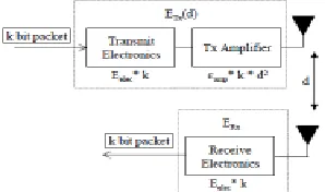
In fact, there are several assumptions in the modeling of the sensor node’s energy consumption (Halgamuge, 2009), (Heinzelman and Balakrishnan, 2000) suggested a theoretical account that contents radio transmission and microcontroller processing. This model was enhanced by the model proposed by Millie and Vaidya (Miller and Vaidya,2005) andthe Zhu and Papavassiliou’s model (Zhu and Papavassiliou, 2003). Diverse assumptions about radio attributes, including energy consumption in transmit and receive modes, will contribute to the strength of these models. In the simulation experiments , we used the radio energy model proposed by Heinzelman(Heinzelman, 2000). The assumptions in the model are:, energy consumption E_XYXZ 50nJ/bit for transmitter and receiver operations is E_XYXZ 50nJ/bit, and for the transmitter amplifieris E_`=a 100pJ/bit/mU for he transmitter amplifier in order to achieve an acceptableE_c.The model is shown in Figure 3.

Figure 3: Radio model energy consumption. Energy consumption during a message transmission is given as;

8EH(, J 8EH;NONP( K 8EH;RST(, J 6

8EH(, J e(. 8NONPK (. 8fghh;RST. J

U _{∶ J idjgkhhklNg}

Where, the threshold J_jgkhhklNg is calculated as in Equation (8).

JjgkhhklNg4 πuL h_λ < hx 8

Next, energy consumption during a receiving,

8LH( 8LH;NONP(

8LH( (. 8NONP 9

Where ( is the message data packet size, 8_EHis the energy model for the transmitter, 8_LHis the energy model of the receiver, 8_NONPis the radio electronics energy, J is the distance between the transmitter and the receiver. All simulation experiments reported in this paper used the model attributes (Heinzelman, 2000) as shown in Table 2.

Table 2: Simulation Model attributes and parameters value.

Sensor field of size M×M meters

This section studiesthe effect network size on the network performance. In this study, the simulation area is varied accordingly. Corresponding base station (BS) location is set and the maximum distance is calculated using Equation (10) as shown in Table 3. The number of nodes is set to 100 with each node offers energy starting at 1 joule. Data packet size is fixed at 512 bytes.

|}~h.R€PN u‚SRH ‚S€UK ƒSRH ƒS€U„ 10

where

‚SRHis the maximum value of X in horizontal axis,

‚S€is the minimum value of X in horizontal axis,

ƒSRHis the maximum value of Y in vertical axis,

ƒS€is the minimum value of Y in vertical axis. Table 3: Max distance with area m xm

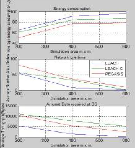
Figure 4 shows the rate of energy consumption, network lifetime and total number of received data at the base station when the sensor field area is varied. The graph shows that the average energy consumption is increased with the increase of network size. Conversely, the total number of alived nodes is reduced with the increment of network size. It is because, with larger network size, more data transmissions need to be delivered to the sink.As the result, the total number of received packets is reduced with the increased of network size due to a higher number of data loss.

Figure 4: Average of energy consumption, number of alive nodes and total number of received data at the BS over different network area size (m x m).

Enhancement of LEACH protocol via selecting the optimum number of clusters

In this section, optimum number of clusters could be used to enhance the performance of LEACH protocol in terms of the total number of alive nodes, average energy consumption and throughput at the base station. Initially, optimum number of clusters are derived by differentiating the expression of E_x>x`Ywith respect to Cand then equating to zero, as shown in Equation (11) (Heinzelman, 2000).

C √Ns

√2π . †

E‡<77;`=a

Ex>ˆ;<`‰;`=a .

M

dU_x>‹Œ 11

where C is the optimum number of clusters, Ns is the number of nodes, M is the simulation area m x m, d_x>‹Œ is the distance from the CH to the base station.

Optimum number of clusters can be calculated analytically using Equation (11) with different parameter values as show in Table 4.

Area m x m BS (X, Y) Max_distance 200 x 200 (11,275) 283 400 x 400 (11,475) 566 600 x 600 (11,675) 849

Parameters Value

Cross-over distance for Friss and two-ray ground attenuation models d_<>77>ŽX<

87 m

Radio Data Rate 1 Mbps

Antenna

Omni-directional

Carrier Sensing Threshold (CSThresh) 1e-9 Watts

Receive Threshold (RXThresh) 6e-9Watts

Energy for Radio Circuitry 50nJoules

Minimum receiver power needed Prthresh for successful reception

6.3 nW

Beamforming Energy 5nJoules/bit

Antenna height above the ground hx , h< 1.5 m

Antenna gain factor Gx , G< 1

Radio amplifier energy E‡<77;`=a 10 pJ/bit/m^2

Radio amplifier energy Ex>ˆ;<`‰;`=a 0.001

3pJ/bit/m^4

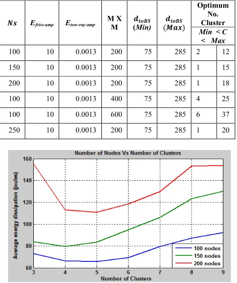
Table 4: Optimum number of clusters with different parameters values.

‘ Efriss-amp Etow-ray-amp M X

M

’“”•–

(Min) ’“”•– —˜™

Optimum No. Cluster Min < C

< Max

100 10 0.0013 200 75 285 2 12

150 10 0.0013 200 75 285 1 15

200 10 0.0013 200 75 285 1 18

100 10 0.0013 400 75 285 4 25

100 10 0.0013 600 75 285 6 37

250 10 0.0013 200 75 285 1 20

Figure 5: Average energy consumption over different number of nodes and number of clusters

Figure 6: Average number of alive nodes over different number of nodes and number of clusters.

Figure 5, Figure 6 and Figure 7 show that the number of nodes N₇of 100 produces the best performance. The best performance of energy consumption, number of alive node and throughput at the base station occurred when the optimum number of clusters is 4 or 5 which is the first row of Table 4. When the number of nodes N₇is 150, optimum number of clusters is in the range between 3 to 5 clusters (the best achieved at 5 clusters), the second row of Table 4, when the number of nodes N₇is 200, optimum number of clusters is in the range 4 - 6 (the best at 5 clusters), which is the third row of Table 4.

Figure 7: Average throughput over different number of nodes and number of clusters.

Effect of the initial energy values per node setting In this section, impact of variation in the initial energy setup on the performance of routing protocols in terms of reliability and scalability is investigated. The initial energy value isset to 1, 2, 3, 5, and 9(joules per node). The number of nodes, packet size, the sensor field size and the base station (BS) location are set to 150 nodes, 512 bytes, 200m × 200m and (11m, 275m) respectively.

Total initial energy Initial energy # No. Nodes12

Figure 8 : Average number of rounds (Time) over different initial energy values for (LEACH.

As seen in Figure 8, the average number of rounds (times) is increased linearly with the increase in the initial energy values per node.

Effect of variation in packet size

In this section, the effect of variation in packet size is studied on the network performance in terms of energy consumption and throughput at the base station.

¡-¢£¡~ _{}J-¨ ¥©££J|§©¥}¤}¢£ ¥-¦£§-¥

where the Packet transmission timeSlot_time TimTxt, The Spread-spectrum packet transmission time,

SSŒY>x­®¯° Slotx=X# spreading

The maximum TDMA frame time can be determined in the following equation:

Frame time SSŒY>x­®¯°# N7

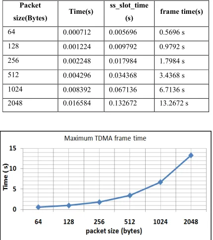
In this part, it is assumed that the bit rate 1Mb; header size 25 bytes, number of clusters is 5 and number of nodes '_his 100 nodes.The nodes is randomly deployed in a sensor field area size of 200m x 200m, with the base station located far away from the sensor field at (11,275). The frame time is computed based on the packet sizes: 64, 128, 256, 512, 1024 and 2048 bytes, as shown in Table 5. The simulation was done using LEACH and PEGASIS protocols.

Table 5: Computed Frame time for different packet sizes

Figure 9: Maximum TDMA frame time over different packet sizes.

Figure 9 shows that that the maximum TDMA frame time is increased with the increase of packet size. The fame time has a direct affect on reliability and quality of wireless communication between nodes. Equation(9) predicts that any increase in packet size k will result in increase energy consumption.

Figure 10: Average throughput over different packet sizes.

Figure 11: Average total energy consumptionover different packet sizes.

Figure10 and Figure11 show throughput and total energy consumption over different packet size respectively. As can be seen on the graphs, the total energy consumption increases linearly with the increase of packet sizes. LEACH consumes more energy when compare to PEGASIS. However, LEACH provides a better throughput compared to PEGASIS. The throughput for both routing protocols are increased with the increase of packet size. This mean,the reliability of data transfer can be improved using a short packet size, which caused less or no error to happen. On the other hand, this scenario is less efficient due to standardized data payload, packet overhead and additional control packets at every node. In most literatures, researchers in WSNs use 512 or 500 bytes as the optimum value for the data packet sizes.

Efficiency of different logical topologies in WSNs

In this section, we focus on evaluation of different logical topologies with their corresponding protocols. The comparisons are made based on cluster–distributed topology, chain topology, cluster-centralized topology and flat topology with their corresponding protocols LEACH, PEGASIS, LEACH-C, and MTE. The performance metrics measured are energy dissipation, number of surviving nodes and throughput at the base station.

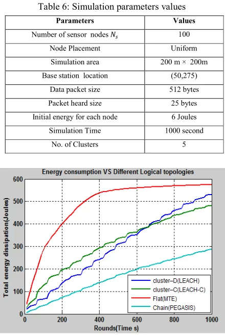
In these experiments, the simulation model attributes are shown in Table1. With a set of the most relevant parametersare shown in Table 6, where the sensor nodes are deployed randomly in the area of 200m × 200m and the base station’s location outside the area at (50,275). The initial energy is set to 6 joules, data packet size is set to 512 bytes, packet header size is set25 bytes and the period of simulation is set to 1000s.

Figure 12, Figure 13 and Figure14, the chain-based topology shows the best performance in therm of total energy consumption, network lifetime and throughput when compared to other types of topology. For a cluster, distributed topology and cluster centralized topology, they located in the middle of the worst, and better performance with an advantage of the cluster centralized topology.

Packet

size(Bytes) Time(s)

ss_slot_time

(s) frame time(s)

64 0.000712 0.005696 0.5696 s

128 0.001224 0.009792 0.9792 s

256 0.002248 0.017984 1.7984 s

512 0.004296 0.034368 3.4368 s

1024 0.008392 0.067136 6.7136 s

Table 6: Simulation parameters values

Figure 12: Total energy consumption for different logical topologies.

Figure 13: Number of alive nodes for different logical topologies.

Figure 14: Throughput for different logical topologies. CONCLUSIONS

In this paper, performances of logical topologies along with their corresponding protocols for WSNs were evaluated, and the impact of various parameters on the efficiency of the protocols in WSNs were studied. The simulation was done using NS-2.34 program with MIT-extension for LEACH, PEGASIS, LEACH-C, and MTE MATLAB was used to plot the graphs. These various parameters are sensor field size M × M, initial energy, optimum number of clusters, and data packet size) . Based on the results obtained from the study, the effect of parameters on the network performance can be concluded as follows:

1 The small sensor area size and a short distance to BS provides the best network performance. The initial energy value for each node has an effect on network reliability, scalability and there prolonging the network's lifetime and increasing the number of rounds (simulation time).

2 Optimum number of clusters depends on the parameters in Equation (11). The optimum number of cluster is 5 clusters.

3 The energy consumption is increased with the increased of packet size. Contrary, the throughput is decreased with the increased of the packet size.The appropriate packet size is 512 bytes.

We infer that from this study the chain logical topology gives a better performance overall logical topologies.

REFERENCES

Dave, P. M., &, P. D. (2013).Simulation & Performance Evaluation of Routing Protocols in Wireless Sensor Network. Simulation, 2(3).

Geetha, V., Kallapur, P. &Tellajeera, S. (2012). Clustering in wireless sensor networks: Performance comparison of leach & leach-c protocols using ns2. Procedia Technology, 4, pp. 163–170.

Parameters Values

Number of sensor nodes 'h 100

Node Placement Uniform

Simulation area 200 m × 200m

Base station location (50,275)

Data packet size 512 bytes

Packet heard size 25 bytes

Initial energy for each node 6 Joules

Simulation Time 1000 second

Halgamuge, M., Zukerman, M., Ramamohanarao, K.and Vu, H. (2009).AN Estimation Of Sensor Energy Consumption.PIER B, 12, pp.259-295.

Heinzelman, W. B. (2000). Application-specific protocol architectures for wireless networks (Doctoral dissertation, Massachusetts Institute of Technology). Heinzelman, W. B., Chandrakasan, A. P., &Balakrishnan, H. (2002).An application-specific protocol architecture for wireless microsensornetworks.Wireless Communications, IEEE Transactions on, 1(4), 660-670.

Heinzelman, W. R., Chandrakasan, A., &Balakrishnan, H. (2000, January).Energy-efficient communication protocol for wireless microsensor networks.InSystem Sciences, 2000.Proceedings of the 33rd Annual Hawaii International Conference on (pp. 10-pp). IEEE. Lindsey, S., Raghavendra, C. &Sivalingam, K.M. (2002). Data gathering algorithms in sensor networks using energy metrics. Parallel and Distributed Systems, IEEE Transactions on, 13(9), pp. 924–935.

Liu, X. (2012).A survey on clustering routing protocols in wireless sensor networks. Sensors, 12(8), pp. 11113– 11153.

Mamun, Q. (2012). A qualitative comparison of different logical topologies for wireless sensor networks. Sensors, 12(11), 14887-14913.

Miller, M. J., & Vaidya, N. F. (2005).A MAC protocol to reduce sensor network energy consumption using a wakeup radio. Mobile Computing, IEEE Transactions on, 4(3), 228-242.

Rajagopalan, R., & Varshney, P. K. (2006). Data aggregation techniques in sensor networks: A survey. Wang, J., Tang, B., Zhang, Z., Shen, J., & Kim, J. U. (2014).Energy Efficient Data Dissemination Algorithm for Wireless Sensor Networks. PP.1-6.