The application of Laser Induced Breakdown Spectroscopy (LIBS) to the analysis of geological samples in simulated extra terrestrial atmospheric environments

(1)

The application of Laser Induced

Breakdown Spectroscopy (LIBS) to

the analysis of geological samples in

simulated extra-terrestrial

atmospheric environments

N. S. LUCAS

(2)

List of Tables

Table 1.1: Pressure and Gaseous environments within the chosen experimental range1-3.

Table 3.1: Doppler and Stark widths from literature34, with electron densities of 1017.cm-3.

Table 3.2: Energy ordering of subshells

Table 3.3: Spectroscopic notation with respect to azimuthal quantum number.

Table 3.4: Pressure values and corresponding mean free paths. (calculated from equation 3.20)

Table 4.1: Table showing wavelength reproducibility errors, Grating 2400g/mm

Table 4.2: Table showing wavelength reproducibility errors, Grating 600g/mm

Table 4.3: Table showing wavelength reproducibility errors, Grating 150g/mm.

Table 6.1: Elemental ratios of constituents in sandstone

Table 6.2: Elemental ratios of constituents in weathered sandstone Table 6.3: Elemental ratios of constituents in pale slate

(6)

List of Figures

Figure 1.1: Illustrative study of LIBS timeline. (Composite drawn from many sources)

Figure 1.2: Image of the atmospheric regions of Titan in comparison to Earth5.

Figure 1.3: Possible present-day structure of Titan’s interior12.

Figure 1.4: Image of Titan’s surface taken by the Huygens lander on January 14th, 200514.

Figure 2.1: LIBS publications by year groupings30

Figure 3.1: Illustration of the pumping arrangement of a Nd:YAG laser. Figure 3.2: Surelite laser optical layout

Figure 3.3: Illustration of possible transitions of electrons. (Composite drawn from many sources)

Figure 3.4: Schematic diagram of plasma propagation34

Figure 3.5: Graph showing matrix effect evident in samples containing both sand and lead80.

Figure 3.6: Saha factors applied to nitrogen99 (pressure=0.1Pa)

Figure 3.7: Energy level diagram for one electron atom. (composite drawn from many sources)

Figure 3.8: Influences on atomic energy levels103.

Figure 3.9: Absorption bands of methane from 750-940nm114 Figure 3.10: Image of total internal reflection inside a optical fibre. Figure 3.11: Illustration of diffraction parameters for a grating.

Figure 3.12: Illustration of diffraction parameters for a blazed grating. Figure 3.13: An image intensifier tube

Figure 3.14: Illustration of timing requirements for LIBS experiments. Figure 4.1: Setup and image of beam profile capture using CCD camera Figure 4.2: Setup and circuit diagram of beam profile capture using

photodiode

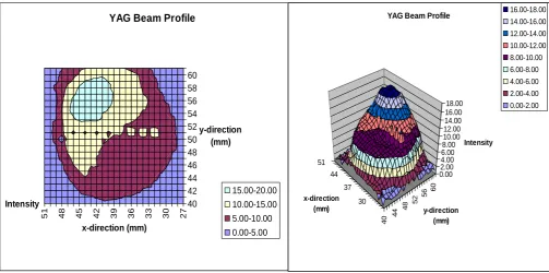
Figure 4.3: Charts showing beam profile from photodiode capture, the different colours represent the beam intensity

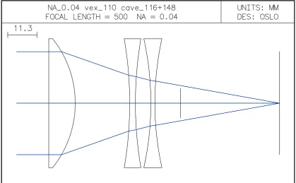
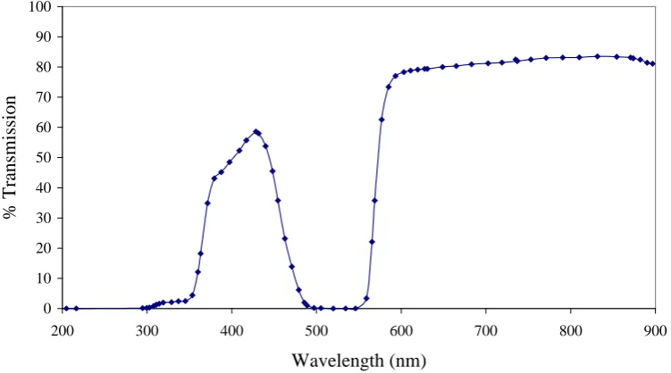
Figure 4.4: Light coupling optics lens setup diagram Figure 4.5: Transmission response of orange perspex.

Figure 4.6: Schematic of the system timing using pulse generator Figure 4.7: Circuit diagram of impedance matching circuit Figure 4.8: Circuit diagram of delay circuit

Figure 4.9: Schematic of the system timing using delay and impedance circuit.

Figure 4.10: Schematic of the system timing, showing redundant parts of system to be removed for calibration.

Figure 4.11: Schematic of the system timing, showing setup with external timing box.

Figure 4.12: Schematic of the final arrangement for the timing setup of the LIBS system

Figure 4.13: Schematic of the final arrangement for the timing setup of the LIBS system, with inherent delays shown.

(7)

Figure 4.15: Grating efficiencies versus wavelength

Figure 4.16: Intensity versus wavelength for gratings corrected for their efficiency wavelength response

Figure 5.1 Working drawings of HPVA chamber

Figure 5.2: Chart showing transmission curve for the HPVA dome.

Figure 5.3: Image to show micrometer feedthroughs of sample stage on the HPVA

Figure 5.4: Image to show sample stage and coupling bracket

Figure 5.5: Image of configuration of fibre bundle at the spectrometer end Figure 5.6: Drawing of optical fibre feedthrough, courtesy of John Cowpe and

Richard Pilkington

Figure 5.7: Image showing alignment of fibre end Figure 5.8: Image showing optical fibre feedthrough Figure 5.9: Schematic of vacuum apparatus setup

Figure 5.10: Schematic of high pressure/vacuum apparatus setup Figure 5.11: Calibration of 100sccm MFC

Figure 5.12: Calibration of 20sccm MFC Figure 5.13: Rate of fill of HPVA

Figure 5.14: Leak rate of vacuum apparatus Figure 5.15: Image of Praxair Bourdon gauge

Figure 5.16: Average of three sets of measurements for calibration of the Bourdon gauge when used at pressures below atmospheric Figure 5.17: Schematic of optical bench setup

Figure 6.1: Graph showing fluctuations in cadmium lamp intensity over time Figure 6.2: Calibration using mercury lamp, 150grooves/mm grating

Figure 6.3: Calibration using mercury lamp, 600grooves/mm Figure 6.4: Calibration using mercury lamp, 2400grooves/mm Figure 6.5: Copper emission spectrum

Figure 6.6: Chart showing fluence at varying distances from the focal point of the final lens

Figure 6.7: Emission intensity versus distance from focal point for CIS and its constituents

Figure 6.8: Spectrometer image of cadmium emission lines

Figure 6.9: Imaged size of spectrometer entrance slit versus actual vernier reading

Figure 6.10: Spectral responses of solder matrix and its constituent parts Figure 6.11: Solder emission spectrum

Figure 6.12: Addition of constituent species emission spectra. (Sn, Pb, Cu, rosin flux)

Figure 6.13: Solder emission spectrum minus lead emission spectrum Figure6.14: Solder emission spectra minus lead and tin emission spectra Figure 6.15: Solder emission spectrum minus lead, tin and copper emission

spectra

Figure 6.16: Solder emission spectrum minus lead, tin and copper emission spectra

Figure 6.17: Shot versus intensity plot to illustrate removal of CIS on silicon substrate, 1.33x108Wcm-2

(8)

Figure 6.19: SIMS comparison of copper, indium and selenium depth distributions

Figure 6.20: RBS plot showing experimental results cross referenced with simulated results

Figure 6.21: Images of ablation crater’s on thin film CIS sample deposited on silicon.

Figure 6.22: SEM image showing an ablation crater

Figure 6.23: Image of silicon sample after laser ablation, the circles are ablation craters.

Figure 6.24: Silicon sample in atmospheric conditions, 150g/mm grating Figure 6.25: Silicon Sample in atmospheric conditions, 2400g/mmgrating Figure 6.26: Images of sandstone samples, with ablation craters clearly visible.

Both were taken from a larger block shown on the left, where organic residues can be seen building up on the surface, the clean stone visible underneath.

Figure 6.27: Sandstone sample emission spectrum in atmospheric conditions, 2400g/mm

Figure 6.28: Slate sample showing ablation craters and re-deposition of material around the crater.

Figure 6.29: Pale slate sample in atmospheric conditions, 2400g/mm grating Figure 6.30: Dark slate sample in atmospheric conditions, 2400g/mm grating Figure 6.31: Pale slate sample in 1 bar nitrogen fill, 2400g/mm grating Figure 6.32: Dark slate sample in 1 bar nitrogen fill, 2400g/mm grating Figure 6.33: Images of marble samples, the one on the left showing the

crystalline structure, the one on the right showing the ablation craters and in some cases the re-deposition from a partial or full methane content atmosphere.

Figure 6.34: Marble sample in atmospheric conditions, 2400g/mm grating Figure 6.35: Marble sample emission spectrum, 1 bar nitrogen fill, 2400g/mm

grating

Figure 6.36: Marble sample emission spectrum, in vacuum as emission lines exhibit self-reversal at other pressures, 2400g/mm grating Figure 6.37: Sandstone EDX image

Figure 6.38: Sandstone EDX image, 4* original magnification to resolve iron and copper peaks.

Figure 6.39: Weathered sandstone EDX image Figure 6.40: EDX Image of marble sample Figure 6.41: Pale slate EDX image

Figure 6.42: Dark slate EDX image

Figure 6.43: Delay variation, silicon sample, atmospheric pressure

Figure 6.44: Delay variation, silicon sample, 1.5 bar pressure of gasmixture 94%N2 6%CH4

Figure 6.45: Delay versus emission intensity of the silicon emission line at 251.61 nm in different samples. Averaged over 15 shots, 1.5 bar pressure with gas mixture 94%N2 6%CH4

Figure 6.46: Delay variation, silicon sample, 1.5 bar pressure of gas mixture 93%N2 7%CH4.

(9)

Figure 6.48: Delay variation, sandstone sample, under vacuum pressure of 5x10-2 mb.

Figure 6.49: Silicon pressure variations, delay 600 ns Figure 6.50: Silicon delay variations, pressure 3x10-4mb Figure 6.51: Silicon delay variations, pressure 4x10-6mb

Figure 6.52: Width variation in microseconds at 1.5 bar with 6% CH4 94% N2

gaseous mixture, silicon sample

gaseous mixture, sandstone sample

Figure 6.57: Schematic diagram of optical bench setup for power variations Figure 6.58: Power output with relation to iris size

Figure 6.59: Power variation (mJ/pulse) on silicon sample, gas composition: 5%CH4 95%N2

Figure 6.60: Power variation (mJ/pulse) on sandstone sample, gas composition: 5%CH4 95%N2

Figure 6.61: Power variation (mJ/pulse) on silicon sample, gas composition: 7%CH4 93%N2

Figure 6.62: Power Variation on Sandstone Sample, gas composition: 6%CH4

94%N2

Figure 6.63: Averaged over 15shots, Power Variation on Sandstone Sample, gas composition: 6%CH4 94%N2

Figure 6.64: Logarithmic plot of power variation, sandstone sample, gas composition: 6%CH4 94%N2

Figure 6.65: Power variation on silicon sample, gas composition: 6%CH4

94%N2

Figure 6.66: Power variation on weathered sandstone sample, gas composition: 6%CH4 94%N2

Figure 6.67: Weathered sample 3D emission spectra, 15 shots Figure 6.68: Weathered sample spectrum, first shot

Figure 6.69: Weathered sample spectrum, fifteenth shot

Figure 6.70: Image of weathered sandstone sample, showing green algae build-up.

Figure 6.71: Weathered surface emission intensity reduction with shot number in atmospheric conditions

Figure 6.72: Comparison of silicon line emission intensity increase with shot number in atmospheric conditions

Figure 6.73: Weathered sample spectrum, first shot at 5x10-2 mb Figure 6.74: Weathered sample spectrum, fifteenth shot at 5x10-2 mb Figure 6.75: Weathered surface lines emission intensity reduction with shot

number at 5x10-2 mb

Figure 6.76: Comparison of silicon line emission intensity increase with shot number at 5x10-2 mb

(10)

Figure 6.78: Weathered sample emission spectrum, fifteenth shot at 1.5 bar nitrogen fill

Figure 6.79: Weathered surface lines emission intensity reduction with 1.5 bar nitrogen fill

Figure 6.80: Comparison of silicon line emission intensity increase with shot number at 1.5 bar nitrogen fill

Figure 6.81: Weathered sample emission spectrum, first shot at 1.5 bar methane fill

Figure 6.82: Weathered sample emission spectrum, fifteenth shot at 1.5 bar methane fill

Figure 6.83: Weathered surface lines emission intensity reduction with a 1.5 bar methane fill

Figure 6.84: Comparison of silicon line emission intensity increase with shot number with a 1.5 bar methane fill

Figure 6.85: Silicon and iron emission line intensity increase with shot number Figure 6.86: Weathered sample emission spectrum, first shot at 1.5 bar,

6%CH4 94%N2 fill

Figure 6.87: Weathered sample emission spectrum, fifteenth shot at 1.5 bar, 6%CH4 94%N2 fill

Figure 6.88: Weathered surface lines emission intensity reduction with shot number, 1.5 bar 6%CH4 94%N2 fill

Figure 6.89: Comparison of silicon line emission intensity increase with shot number, 1.5 bar 6%CH4 94%N2 fill

Figure 6.90: Single shot emission spectrum of silicon sample showing intensity change with pressure, with N2 as filling gas

Figure 6.91: 15 shot average, silicon sample, intensity change with pressure, with N2 as filling gas

Figure 6.92: Silicon sample emission intensity change with pressure, with 5%/95% mixture as filling gas, variation in millibar

Figure 6.93: Silicon sample emission intensity change with pressure, with 6%94% mix as filling gas, variation in millibar

Figure 6.94: Simplified silicon sample emission intensity change with pressure, with 6%94% mix as filling gas, variation in millibar

Figure 6.95: Silicon sample emission intensity change with pressure, with 7%/93% mixture as filling gas, variation in millibar

Figure 6.96: Silicon sample emission intensity change with pressure, with CH4

as filling gas, variation in millibar

Figure 6.97: Sandstone sample emission intensity change with pressure, with N2 as filling gas, variation in millibar

Figure 6.98: Sandstone sample emission intensity change with pressure, with CH4 as filling gas, variation in millibar

Figure 6.99: Sandstone sample emission intensity change with pressure, with 6%/94% mix as filling gas, variation in millibar

Figure 6.100: Simplified sandstone samples emission intensity change with pressure, with 6%94% mix as filling gas, variation in millibar Figure 6.101: Chart showing emission intensity change with pressure, with N2

as filling gas, silicon sample.

(11)

Figure 6.103: Change in emission intensity with pressure variations , 6/94 mix as filling gas, silicon sample

Figure 6.104: Change emission intensity with pressure variations, 7/93 mix as filling gas, silicon sample

Figure 6.105: Change emission intensity with pressure variations, CH4 as filling

gas, silicon sample.

Figure 6.106: Plot of specific emission line intensity variations from each sample with respect to pressure.

Figure 6.107: Silicon sample, emission signal with different gaseous content at 1.5 bar

Figure 6.108: Silicon sample, carbon line emission signal with different gaseous content at 1.5 bar

Figure 6.109: Silicon sample, carbon emission intensity for various gas fills Figure 6.110: Silicon sample, carbon and silicon emission intensities for various

gas fills

Figure 6.111: Plot of silicon and carbon emission intensities from silicon sample, normalised to silicon.

Figure 6.112: Sandstone sample, carbon and silicon emission intensities for various gas fills

Figure 6.113: Plot of silicon and carbon emission intensities from sandstone sample, normalised to silicon

Figure 6.114: Marble sample, carbon, silicon and oxygen emission intensities for various gas fills

Figure 6.114: Plot of silicon, carbon and oxygen emission intensities from marble sample, normalised to silicon

Figure 6.115: Emission intensities of various marble emission lines showing variations due to pressure and gaseous content

Figure 6.116: Pressure variation of Ca(II) 393.37nm and Ca (II) 396.85nm in marble, with N2 fill. Showing self reversal due to pressure.

Figure 6.117: Simplified Pressure variation of Ca(II) 393.37nm and Ca (II) 396.85nm in marble, with N2 fill. Showing self reversal due to

pressure.

Figure 6.118: Pressure versus intensity variation of calcium emission lines from marble sample, with nitrogen filling gas.

Figure 6.119: Image of dark slate sample showing ferrous reduction spheres. Figure 6.120: Image of slate sample showing ‘sooting’ of the surface from

re-deposition at the ablation craters.

Figure 6.121: Pale slate, emission intensity change with pressure variations, nitrogen filling gas, wavelength centre at 252nm.

Figure 6.122: Pale slate, emission intensity change with pressure variations, nitrogen filling gas, wavelength centre at 276nm.

Figure 6.123: Dark slate, emission intensity change with pressure variations, nitrogen filling gas, wavelength centre at 252nm.

Figure 6.124: Dark slate, emission intensity change with pressure variations, nitrogen filling gas, wavelength centre at 276nm.

Figure 6.125: Pale slate, pressure versus intensity variations with nitrogen filling gas

(12)

Figure 7.1: One standard deviation of delay versus emission intensity of the silicon emission line at 251.61 nm in different samples. Averaged over 15 shots, 1.5 bar pressure with gas mixture 94%N2 6%CH4

Figure 7.2: One standard deviation of power versus intensity variations on sandstone sample, gas composition: 6%CH4 94%N2

Figure 7.3: One standard deviation of change in intensity with pressure, with N2 as filling gas, silicon sample.

Figure 7.4: One standard deviations of change in intensity with pressure, with 6/94 mix as filling gas, silicon sample

(13)

Acknowledgements

I would initially like to thank all those I worked closely with in the Laser Group at Salford University. To Richard Pilkington for his help and his enthusiasm with P.L.O.P. and Christmas escapes to the country. Robin Hill, without his help to pull it out of the bag I would never have submitted my thesis. Stuart Astin for his kindness of heart and quiet unassuming knowledge and patience with lessons. Helen Brown for mutual expulsion of stress and ‘ciggie break’ escapes. To John Cowpe for his knowledge on vacuum apparatus and systems and to Garry Rowsell for his ‘think tank’ help.

Thanks must go to other staff at Salford University. Jay Smith, for his ingenuity. Steve Hurst and Mike Hulme for their workshop ‘wizardary’. To Bruce (and the voices) and Paul Murphy for their PC know how. Graham Keeler and Brian James for their computer programming and interfacing help. Allan Boardman for his valuable support. Dave armour for his guidance on plasma processes and Keren Maloney for her help and patience with administration support.

External to the university I would like to thank Nigel Murphy and John Wilkinson at Universal Imaging Corporation for their continued support throughout the project.

I give thanks to EPSRC for my funding. I also would like to thank the institutions who made it possible for me to attend conferences with their generous financial support, namely; The Rank Prize Funds; The European Space Agency, The International Astronautics Federation and to Dave Wright of the British Rocketry Oral History Programme.

(14)

Not least I give thanks to my family, without their help, support and love I would have never achieved such dizzy heights!

Declaration

(15)

Abbreviations

ADC Astronomical Data Centre CCD charged-coupled device

CF-LIBS calibration free laser induced breakdown spectroscopy CIS copper indium diselenide

EDX X-Ray dispersive analysis EPROM electronic prompt

ESA European Space Agency FO optical fibre

HPVA high pressure/vacuum apparatus

IBM International Business Machines Corporation ICCD intensified charged-coupled device

KTP potassium titanyl phosphate LANL Los Alamos national laboratory

LASER light amplification by stimulated emission of radiation LED light emitting diode

LIBS laser induced breakdown spectroscopy LOD limit of detection

LSAW laser-supported absorption wave LSCW laser-supported combustion wave LSDW laser-supported detonation wave LSRW laser-supported radiation wave LTE local thermodynamic equilibrium LTSD lens to surface/sample distance MCP micro-channel plate

MFC mass flow controller MFP mean free path MUT material under test

NASA National Aeronautics Space Administration Nd:YAG neodymium: yttrium-aluminum-garnet

NIST National Institute of Standards and Technology PCB printed circuit board

PTG programmable timing generator RBS Rutherford Backscattering SEM scanning electron microscope SIMS secondary ion mass spectrometry TEM00 fundamental transverse mode

UV-VIS ultraviolet-visible

(16)

Abstract

Laser induced breakdown spectroscopy (LIBS) is a technique that can determine the elemental composition and quantities of a sample by the spectral analysis of a laser induced plume.

This study was undertaken to develop, characterise and assess the use of the LIBS technique on geological samples in different pressure and gaseous environments. The experimental range chosen was dictated by the planetary conditions on Titan and other extra-terrestrial bodies with the samples analysed chosen to complement a range of rock types.

A LIBS system was developed, together with associated experimental apparatus able to acquire results in varying pressure and gaseous environments. The capability of LIBS to analyse weathered rock samples was investigated under various ambient conditions; pressures of 160x103 Pa to 0.4x10-3 Pa and ambient gaseous mixtures of air, nitrogen and methane.

Particular attention was paid to temporal and power considerations under such regimes. As was expected, the chosen delay time to optimise the emission signals needed to be increased with increasing ambient pressure. At power values as low as 28.5 mJ/pulse (using a 6 ns pulse from a doubled Nd:YAG laser at 532 nm) a valid emission signal could be obtained. Increasing the laser power resulted in a reduction in the overall signal to noise ratio.

It was observed that ambient methane quenches the optical emission signal due to non-radiative transitions. In spite of this, valid qualitative data are obtainable, even when emissions due to carbon transitions from both the sample and the gaseous environment, are present.

(17)

1. Introduction

1.1 Background

The main thrust of this research study was to fully commission a laser induced breakdown spectroscopy (LIBS) system for use at Salford University. This equipment was developed to incorporate apparatus able to analyse LIBS in varying pressure environments.

Once commissioned a study was undertaken to examine the effects of pressure and different gaseous environments on the LIBS technique, paying particular attention to temporal affects and power considerations. The environments chosen varied from pressures of 160x103 Pa to 0.4x10-3 Pa with different gaseous mixtures of air, nitrogen and methane.

This work was personally carried out from conception to completion, with a view to ascertaining the ability of the LIBS technique to acquire good analytical data in the atmosphere of the moon Titan, a previously unexplored experimental environment.

LIBS is a technique that can determine the elemental composition and quantities of a sample by analysis of emission from a laser induced plume. A high power laser is focused onto the material of interest creating a plume; this plume expands over time and spectral emissions result from the relaxation of the constituent excited species. The atomic spectral lines are then used to analyse the material.

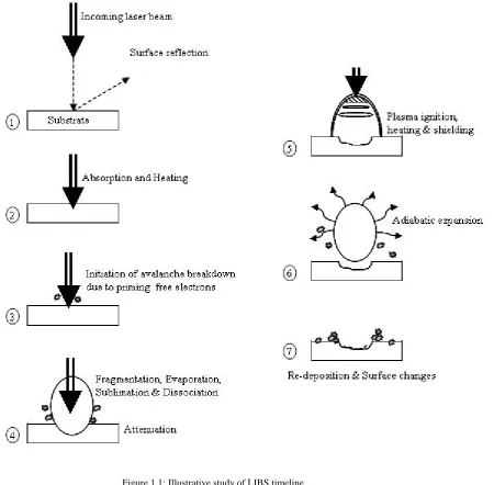
The timeline involved in LIBS analysis can be broken down and summarised, illustrated in figure 1.1, each section being explained in greater detail in the following theory chapter.

1) Incidence of the laser pulse upon the sample.

2) Absorption and heating of the sample via the incident laser energy 3) Priming electrons initiate the laser ablation process

(18)

5) The plume itself acts to shield the sample surface from the remaining incident laser light.

6) After the laser pulse finishes the plume expands away from the surface 7) Once the plume has dissipated some constituents may be re-deposited on

[image:18.595.108.559.246.688.2]

the sample surface.

(19)

1.2 Planet and Moon Environments

The experimental range chosen accounted for the atmospheric conditions on varying moons and planets in our solar system, paying particular attention to that of Titan, one of the moons of Saturn.

LIBS is of particular interest for space applications due to its capability for use at stand-off distances, thus eliminating the possibility of cross contamination of samples. Titan is one of the moons of Saturn and of particular importance as it is the only known moon with a fully developed thick atmosphere that is rich in organic compounds. As such Titan may be a clue as to how life began on Earth.

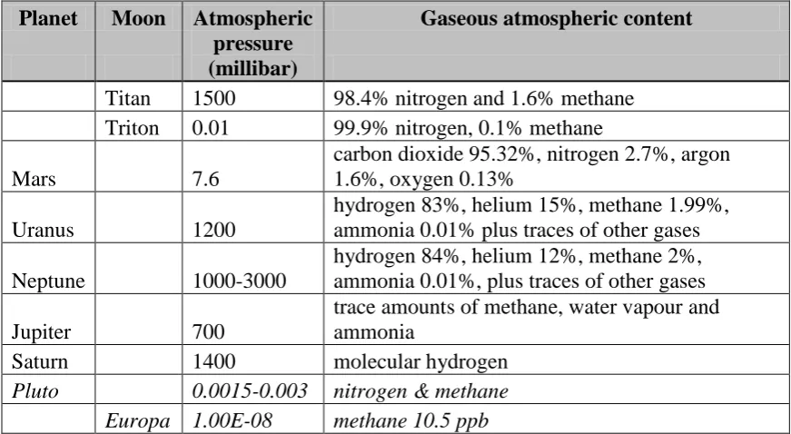
[image:19.595.107.543.455.694.2]

Planets and moons that lie within the experimental parameters used in this study are shown in table 1.1. As can be seen, many atmospheric pressures fall within the experimental range, as do some gaseous atmospheric contents. As such the results obtained in this study could prove valuable for many extra-terrestrial applications.

Table 1.1: Pressure and Gaseous environments within the chosen experimental range1-3.

Planet Moon Atmospheric Gaseous atmospheric content

pressure (millibar)

Titan 1500 98.4% nitrogen and 1.6% methane Triton 0.01 99.9% nitrogen, 0.1% methane

Mars 7.6

carbon dioxide 95.32%, nitrogen 2.7%, argon 1.6%, oxygen 0.13%

Uranus 1200

hydrogen 83%, helium 15%, methane 1.99%, ammonia 0.01% plus traces of other gases Neptune 1000-3000

hydrogen 84%, helium 12%, methane 2%, ammonia 0.01%, plus traces of other gases Jupiter 700

trace amounts of methane, water vapour and ammonia

Saturn 1400 molecular hydrogen Pluto 0.0015-0.003 nitrogen & methane Europa 1.00E-08 methane 10.5 ppb

(20)

Previous studies have been undertaken to ascertain the capability of the LIBS technique in Martian, Venetian and the low pressure environments of moons and asteroids. These are described in sections 2.3 and 3.7.

These reports have been so successful that missions have been plannedI1 incorporating a LIBS instrument for analysis of rocks and soils on the Martian surface. The first mission is being planned for launch in 2009, on board the NASA’s Mars Science Laboratory and the second, a LIBS-Raman combined instrument, is being planned to launch in 2011 by the European Space Agency on the ExoMars rover mission.

To complement these studies this research was aimed at Titan, to establish if this technique can also be used in this distinct and currently un-explored environment.

Since this study was undertaken, new data has been acquired from a mission to Saturn and Titan. The spacecraft in this mission is called Cassini-Huygens, and it reached Saturn on July 1, 2004, the first Huygens data being reported by ESA on January 21st 2005.

Previously Titan had been examined by the space missions Voyager 1 and Voyager 2. Voyager 1’s mission had been diverted specifically to make a closer pass of Titan, but unfortunately this mission’s instrumentation range did not include an instrument that could penetrate Titan’s haze.

(21)

Figure 1.2: Image of the atmospheric regions of Titan in comparison to Earth5_.

Titan’s atmosphere is now known to contain 98.4% nitrogen and 1.6% methane, but this methane content is known to increase to 5% near the surface and there has been indication that the surface landing site of the Huygens probe was soaked in methane6.

The amount of methane abundant in Titan’s atmosphere is somewhat a mystery as the solar winds in the early solar system should have cleared the atmosphere of methane content. Leading theories believe that in early formation, methane was frozen as water-ice or ‘clathrates’ which have since melted releasing methane into the atmosphere.

At the time of implementation of experimentation, (before the Cassini-Huygens mission data was obtained on atmospheric composition), the compositional content of Titan was thought to be 94% nitrogen and 6% methane. A percent variance of these compositions was covered in the experimental parameters.

(22)

1.3 Rock Composition

[image:22.595.401.566.98.295.2] [image:22.595.116.275.345.660.2]

At the time of experimentation, the types of rock found on Titan were virtually unknown. It was thought that there were seas of liquid hydrocarbons7 and that Titan’s bulk composition was water ice with approximately 65% rock-metal material8. It was proposed that Titan was dense due to its gravitational compression9 and its structure was differentiated into several layers composed of different crystal forms of ice10 and that its interior may once have contained a hot liquid layer consisting of water and ammonia between the ice crust and the rocky core11.

Figure 1.3: Possible present-day structure of Titan’s interior12.

Taking into account these suppositions, rock types were chosen with a range of composition elements of metamorphic rock types. Slate was chosen as a foliated metamorphic rock type. Marble was also chosen as a metamorphic calcite rock.

Subsequent to choosing the above rock types further information was obtained via radar from the Cassini spacecraft13. This information conflicted with information previous thoughts that there were seas of hydrocarbons at the equator. Radar images revealed that these regions were in fact extensive plains covered in longitudinal sand dunes. As a result of this information sedimentary sandstone was also chosen for testing.

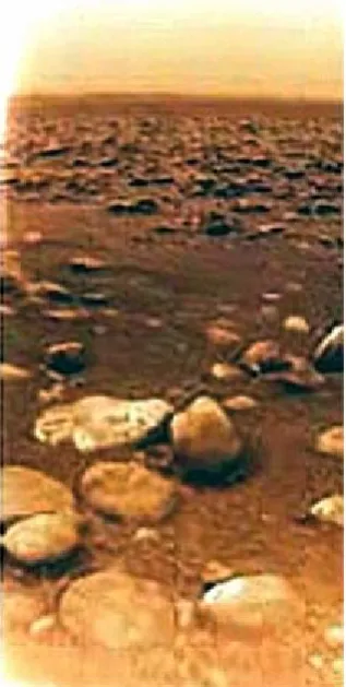
Figure 1.4: Image of Titan’s surface taken by the Huygens lander on January 14th, 200514.

Figure 1.3: Possible present-day

structure of Titan’s interior12.

Figure 1.4: Image of Titan’s surface taken by the Huygens lander on January

(23)

(24)

2. History and Uses

2.1 Scientific History of LIBS

LIBS was first published in the report by Brech and Cross in 1962, which observed emission spectra from a metal target using a ruby maser15. In 1963 the paper published by Debras-Guédon and Liodec16 described first analytical use of LIBS using a ruby laser to produce excited spectral emissions of the elements. In 1964 the first use of a Nd:YAG laser was reported by Geusic17 et al from Bell Labs. In the same year Maker, Terhune and Savage18 reported the first observation of optically-induced breakdown in a gas.

In the early 1970’s Moenke-Blankenburg19 wrote a review on LIBS with cross-excitation, and in the late 1980’s the same author produced the book ‘Laser Microanalysis20’, which also provided another comprehensive review of the analytical applications of laser-target interactions.

(25)

In the 1980’s only a handful of groups were working on LIBS; this number has increased exceedingly since then, as shown in figure 2.1.

Figure 2.1: LIBS Publications by year groupings30

In the late 1990’s, with the advent of high resolution spectrometers, the LIBS technique really took off. These detectors allowed multiple elements to be detected at once, with increased sensitivity compared to that of previous methods.

The first international conference on LIBS was held in 2000 in Pisa, Italy. Since this date conferences have been held yearly, each alternate year being an international meeting.

A comprehensive LIBS review paper was written by D. Cremers31 and L Radziemski in 1987, and another was written in 2002 by L. Radziemski32, which provides a sense of the technique’s development from inception to the year 2000.

Another thorough review focusing on the effects of experimental parameters on LIBS analytical performance was provided by E. Tognoni33 et al, early in 2002. This paper refers to literature of experimental studies from 1988 to 2001.

Lastly, a useful source for the all-inclusive history of LIBS is the Handbook of Laser Induced Breakdown Spectroscopy34, which provides a broad review from 1960 – 2002.

Figure 2.1: LIBS publications by year groupings30

8 15

36

203

0 50 100 150 200 250

81-85 86-90 91-95 96-2000

Years

N

um

be

r of

P

ubl

ic

at

(26)

2.3 Uses, Types and Divisions

LIBS analysis is extremely versatile and can be used in many different fields of research. The LIBS technique offers: rapid analysis - one measurement per laser pulse; sampling of solids, gases or liquids; simultaneous multi-element detection; a spatial resolving power of ~1-500 µm; remote analysis capabilities; depth-profiling of layered structures and surface coatings; detection limits of 1-100 ppm, depending on sample composition and instrumental characteristics; all with little or no sample preparation.

Some of the disadvantages of LIBS range from poor shot-to-shot stability; matrix effects; poor signal to noise ratio; loss of weaker lines and difficulty in obtaining quantative analysis.

There are many different applications of the LIBS technique in numerous different fields. These wide ranging applications include: archaeological analysis of Minoan dagger history35, elemental composition of artworks to characterise pigments in a Byzantine work layer by layer36, analysis of bobsleigh runners in the 2002 winter Olympics to ensure they meet with the Olympic standards in having a homogeneous metallic composition throughout37, various different varieties of coating analysis such as Lademann’s investigation into the stability of coated titanium microparticles used in sunscreens38, dentistry applications, utilizing the high spatial resolutions possible with LIBS, to identify the transition from carious (unhealthy) tissue to healthy tissue39, and in the nuclear industry for remote chemical analysis, exploiting the ability of LIBS to work in submerged remote environments40,41. These several uses mentioned are just a small selection that have so far been explored using the LIBS analysis technique.

(27)

A cross section of papers written by Los Alamos national laboratory (LANL) on LIBS publications for planetary science are stated in Appendix [B] some

reference summaries are stated here:

LIBS Operation on Airless Bodies4,42, a study undertaken to characterise the changes to the LIBS plasma spark in different pressure regimes.

LIBS Operation on Venus4,43, these studies concentrate on the hostile environment of Venus with atmospheric pressures ~90Bars.

Investigation of LIBS feasibility for in situ planetary exploration: An analysis on Martian rock analogues44

This latter study focuses on volcanic rock analysis in an environment similar to a Martian one, using the calibration free LIBS (CF-LIBS) method at wavelengths of 355 nm. It suggests that the technique can be used to allow elemental qualitative and quantative identification on the silicate minerals studied in the Martian environment. The CF-LIBS technique was shown to be accurate within the range 1-30% for the major constituents, but this depended heavily on the element and its concentration. The accuracy would be reasonable for first line identification but could be questionable when used in precise analytical measurements.

LIBS application for analyses of Martian crust analogues: Search for the optimal experimental parameters in air and CO2 atmosphere45.

This study compares a Terrestrial environment to a Martian environment, with particular attention paid to the optimal experimental parameters such as emission intensity, temperature and electron density. It found that the acquisition window where local thermodynamic equilibrium (LTE) holds is much shorter in Martian environments due to low electron density and fast plasma cooling and decay, the latter giving a short interval for maximizing signal to noise ratios.

(28)

3. Theory

The following section will concentrate on each of the processes involved in LIBS analysis. In order to facilitate easy categorisation of the development of the theory, it has been broken down into subsections entitled; Laser; Induced; Breakdown; and Spectroscopy. Following this a thorough investigation of other features in LIBS analysis is undertaken.

3.1 Laser

Theodore Maiman invented the first laser in May 196046. Laser action is initiated by exciting the electrons of the atoms in a laser medium from the ground state into a higher energy level using optical amplification47, producing a population inversion46. This is achieved by pumping48 the laser medium via the application of a large amount of energy in the form of broadband light.

As the electrons make transitions back to the ground state they emit radiation. Most energy transitions emit a phonon, but some transitions result in the emission of a photon. When a photon is emitted it is trapped within the laser cavity. This photon passes through the medium and stimulates further emissions from the population inversion.

There are many types of lasers that can be used in LIBS experiments, examples being Nd:YAG, Excimer, CO2 and Microchip lasers. The majority of LIBS

measurements use a flashlamp pumped Nd:YAG laser, which is the laser used in this work.

The Neodymium-YAG (Nd:YAG) laser rod is a doped insulator laser that uses a Nd3+ion to dope a yttrium-aluminum-garnet host crystal47.

Nd:YAG lasers operate via a four energy level system with the lasing transition taking place between the 4F3/2 and 4I11/2 states48 resulting in infrared light

(29)

interactions from the third level into the second level of this system which is known as a metastable state, meaning that it can return to a less excited state only via a highly inhibited transition. As such, electrons remains in this state for an appreciable fraction of a second rather than for the lifetime of a typical transition rate of ~10-8s. It is this long lifetime that provides the mechanism by which a population inversion can be achieved.

The Nd:YAG laser is a popular choice for laser ablation experiments as it displays a high spatial coherence and has high output energies49.

Converting the 1064 nm laser output to shorter wavelengths is achieved by passing the laser beam through a non-linear crystal. This produces harmonics obtained from phase matching48. The conversion efficiency is approximately 50% and reduces with each harmonic. The crystal used to produce green light of wavelength 532nm, used in this work, is KTP (potassium titanyl phosphate).

The light emitted by a laser will have different optical frequencies associated with different modes of the optical resonator. These resonator modes are known as longitudinal and transverse modes. The longitudinal modes of a laser govern the spectral characteristics, such as line width and coherence length. The transverse modes govern the beam divergence, beam diameter and energy distribution.

A laser that operates in its fundamental transverse mode, or TEM00 mode, emits

light with a Gaussian intensity profile. This light will propagate as a directional

parallel beam for a distance given by πd2_{/λ, the Rayleigh range, (where d is the}

(30)

3.2 Induced (Laser Ablation)

R. Srinivasan and V. Mayne-Banton of IBM Research first reported the laser ablation phenomenon to produce thin films in 198250. Laser ablation is a process whereby the short, intense burst of energy delivered by a laser pulse is used to vaporise a material that would often be impossible to vaporise by conventional methods51,52. Lasers are advantageous in many ways. Because of their high spatial coherence they may be focused onto a very small area and this can result in intense local heating without neighbouring areas being affected. The majority of the laser energy is deposited near the surface of the target, allowing surface regions to be ablated without affecting the bulk. It is also relatively easy to control a laser’s energy density or fluence53.

Fluence (Jcm-2) = laser pulse energy (J) / focal spot area (cm2) (3.1)

Radiant Power or Flux (W) = pulse energy (J) / pulse duration (sec) (3.2)

Intensity or Irradiance (Wcm-2) = peak power (W) / focal spot area (cm2) (3.3)

It is almost impossibly complicated to carry out a detailed theoretical analysis of the ablation process, especially when the substrate melts or vaporises54. However it is possible, making simple assumptions, to adopt models that enable important parameters to be identified and orders of magnitude estimated. Appendix [C] lists some of the most representative theoretical models of the laser-solid interaction, and a brief description of each.

(31)

Laser ablation results in heating and damage to the surrounding area, the degree of which is determined by the rate of energy absorption and the rate of energy loss through thermal conduction in the substrate. In general three types of absorption must be taken into account, volume absorption by the electrons and phonons in the lattice, free carrier absorption at the surface and absorption by the plume.

For ablation to take place there needs to be sufficient heating of the substrate to take it through to the vapour phase. The vaporised material will expand in the form of a plume, the plume being plasma-like, consisting of molecular fragments, neutral particles, free electrons and ions, and chemical reaction products53. The laser energy will continue to heat this partially ionised evaporated material while part of the energy continues to the substrate surface. As the energy increases the plume can become opaque and shield the surface.

The ability of a material to absorb laser energy limits the depth to which that energy can perform useful ablation. Generally, reflectance decreases with decreasing wavelength48. This would tend to suggest that shorter wavelengths would be optimum for ablation, but the reflectance of most surfaces reduces during a laser pulse as the temperature rises. Therefore the initial advantage of a shorter wavelength is not necessarily maintained. For a more detailed study refer to Anisimov et al56 who have taken the reflection of light from substrates and the temperature dependence of the reflectance into consideration.

(32)

In general one can estimate the minimum power density needed to produce vaporisation using the Moenke-Blankenburg57 equation:

2 / 1

2 / 1 min

t L

I v

∆

= ρ κ (3.4)

Where:

Imin = minimum power density (W.cm-2) ρ = density of substrate (kg.m-3)

Lv = latent heat of vaporisation (kJ.kg) ∆t = laser pulse length (s)

κ = thermal diffusivity of specimen (W.m-1.K-1)

The ablation depth per pulse can be calculated using equation34:

(

)

(

)

[

p b v

]

ρ

d

L T T C

R f A

+ −

− =

0

1

(3.5)

Where:

Ad = ablation depth per pulse (m) R = fractional surface reflectivity

Cp = specific heat (J.kg-1.K-1) Tb = boiling point (K)

f = fluence (J/m-2) T0 = room temperature (K)

There will be a significant change in ablation rate when working in different pressure environments, a decrease in pressure producing an increase in ablation rate, due to reduced shielding of the sample surface from the incident laser pulse. Work by Multari et al58, Vadillo et al59 and Semerok et al60, studied factors related to ablation rate, such as fluence, laser pulse length, pressure, lens to surface distance (LTSD) and angle of incidence.

(33)

Multiphoton absorption62,63 is a process that was predicted theoretically by Maria Göppert-Mayer in 1929, but was unable to be experimentally verified until the advent of the laser in 1960. In this process an atom may absorb two or more photons simultaneously, (or within less than a nanosecond), in some cases allowing it to be ionized by photons with an energy less than that of the threshold energy due to possible transitions to virtual states.

Avalanche breakdown is the process whereby an energetic carrier creates a carrier pair after colliding with the lattice. These new carriers are then energised by photon absorption and accelerated until the process repeats and an avalanche develops. A study of avalanche breakdown in air has been completed by Kroll and Watson64.

Avalanche breakdown requires the presence of some “priming” free electrons which can be provided by dust particles, by multiphoton ionisation of a gas atom in the beam path or by absorbed impurities in the substrate which are evaporated and ionised below the bulk substrate threshold.

The vapour particles escaping the substrate surface have a Maxwell velocity distribution with vectors pointing away from the surface65. These vectors are changed by collisions with the vapour particles themselves producing a region known as the Knudsen layer66. Within this layer the plume reaches internal equilibrium and rapidly moves away from the sample surface. If the vapour pressure of the plume within this layer exceeds the ambient pressure, the flow velocity becomes supersonic and forms a shock front. Anisimov et al67 has produced a detailed discussion of vapour expansion and condensation.

(34)

When the plume is partially ionised laser light is absorbed via two methods; by thermally excited atoms (bound-free absorption), and by ions (Bremsstrahlung absorption)61. The Bremsstrahlung phenomenon was discovered by Nikola Tesla in research between 1888 and 189768,69. Bremsstrahlung or ‘braking radiation’, also known as free-free radiation, is the process whereby electromagnetic radiation is produced by the deceleration of a charged particle, in this case an electron, when it has collided with another charged particle, in this case an ion. When this process is reversed, and produces an acceleration of the charged particle, is known as inverse-Bremsstrahlung.

Transitions, (radiation or absorption) that an atom or ion can undergo can be summarised using the following diagram:

Where, from left to right we have:

• bound-bound

• free-bound (Avalanche)

• free-free (Bremsstrahlung)

• Ionisation from the ground state

• Ionisation from an excited state

(35)

Once the plume is fully ionised light absorption is dominated by Bremsstrahlung absorption. In this scenario the plume absorbs all or part of the incident radiation and the energy provided is converted into internal energy of the plume. This energy is consumed as hydrodynamic motion or radiated away as thermal radiation. As mentioned, the plume rapidly expands away from the surface, but this plume also remains confined to a channel formed by the incident light due to interaction of this light with the plume34. This phenomenon is commonly referred to as a Laser-Supported Absorption Wave (LSAW). This wave propagates in three zones, plume front, shock front and absorption front as shown in figure

3.334,70,71.

This LSAW can be divided into two classes depending on the incident irradiance, optical density and internal energy of the plume. The first class, known as a Laser-Supported Combustion Wave (LSCW), is a weakly absorbing subsonic wave, the theory of which was formulated by Raizer in 197072.

The layers of cold gas in the plume front are heated by conduction and thermal radiation from the absorption front until they themselves start producing their own radiation. In this regime a fraction of the light absorbed produces the chemical reaction and the propagation is limited to the laser beam channel, both towards and away from the laser source. The wave is also optically thin so the

(36)

laser radiation can still reach the surface. The velocity of the LSCW scales with the square root of the irradiance and vanishes at critical irradiance61.

The second class of an LSAW is known as a Laser-Supported Detonation Wave (LSDW). In this class the irradiance increases and in consequence there are increases in the temperature, pressure and velocity of the absorption front. The increased irradiance also results in a larger proportion of the beam flux being absorbed, which in turn contributes to preheating and ionization, and ultimately results in the dominating mechanism of plume expansion becoming compression rather than conduction so that the plume front becomes optically thick. The velocities increase and the wave becomes a supersonic shock wave. The plume is also shown to propagate cylindrically along the beam path due to its mechanism being supported by the laser beam.

At even higher irradiances the wave class changes to what is known as a Laser-Supported Radiation Wave (LSRW), or breakdown wave. In this regime the plasma itself is emitting enough radiation to enable the atmosphere in front of it to become absorbing34. This couples the absorption zone to the plasma front. The propagation of this wave relies on avalanche breakdown, with the avalanche first developing at the focal point (region of highest flux) and then transferring that propagation to areas of lower flux.

A one dimensional approximation study of velocities, pressure, temperature and densities for all classes of laser supported waves has been carried out by Root73 in 1989 and a further study modelling ablation mechanisms, rates and analytical considerations is reported by Bogaerts et al74.

(37)

Review papers have been written by Bogaerts et al74 and Russo et al75, which review the many models of the ablation process with varieties of laser and sample parameters. Papers by Aguilera and Aragon76, Wood et al77, Iriarte et al78, Capitelli et al79 and Gizzi et al80 also provide a good understanding of the ablation/plume process within a LIBS plasma.

3.3 Breakdown

(Plasmas)

‘After termination of laser pulse plasma loses energy and decays. Mechanisms include recombination, radiation and conduction…’34

Plasmas produced by laser ablation will expand rapidly and show large density and temperature gradients along the axis of the incoming beam. Typically, plasmas produced in LIBS experiments initiate with high ionisation but after recombination and relaxation the plasma becomes weakly ionised. Throughout this process there is broadband background radiation due to Bremsstrahlung radiation that decays early in the plasma lifetime. The plasma lifetime is only of interest for LIBS experiments when it reaches the later stages, where the recombination radiation is emitted.

LIBS plasmas should preferably be optically thin: an optically thin plasma is a plasma in which the radiation that has been emitted escapes without noteworthy absorption or scattering.

Ideally LIBS plasmas should have an elemental composition identical to that of the substrate. This is not always the case due to the differing volatilities of the constituent species of the substrate producing preferential ablation rates.

(38)

[image:38.595.169.439.148.349.2]

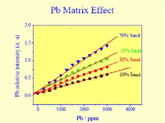
For example, figure 3.4 shows that, although the concentration of lead in the sample is constant, its LIBS analysis shows an incongruent quantity, depending on the matrix composition of lead and sand.

Figure 3.5: Graph showing matrix effect samples containing both sand and lead81.

Many factors influence the degree of fractionation such as laser wavelength, pulse duration and irradiance, fluence and atomic mass of the constituents, as have been extensively studied by Russo et al75,82, Mao et al83, Figg and Kahr84, Jeffries et al85, Eggins et al86, Gunther et al87,88 and Singh and Narayan89. It has been indicated42 that matrix effects are less prominent at lower pressures, due to the reduced proximity of the plasma species resulting in increased interaction between the laser pulse and the sample.

In order to maximise stoichiometry all constituents should be completely vaporised and removed. This can be done by ensuring the energy deposited into the substrate is greater than the latent heat of vaporisation for all matrix constituents. It has been noted by Ready90 that if the irradiance is <106Wcm-2 with microsecond pulse lengths then thermal effects will influence the process allowing differential ablation, but for nanosecond laser irradiances >109Wcm-2 the ejected material should be close to the sample composition due to the thermal properties no longer playing a major role. Bogaerts el al91 provide a review of the laser ablation/plume process with varying models and sample parameters.

Figure 3.5: Graph showing matrix effect evident in samples

(39)

When an electron undergoes a transition to a state of lesser energy it can emit a photon. These photons produce spectral lines characteristic of the atom, ion or molecule. Spectral lines emitted from a plasma have widths, shapes and intensities that depend on the temperature, pressure and electron density of the plasma. Therefore spectral lines can give information about the conditions in the plasma itself. Lines that have been emitted from a ground level transition are in most cases the strongest lines, known as resonance lines.

If a spectral line has changed from its expected value in some way this suggests a perturbation in the medium. This could be a spectral line broadening or shifting mechanism due to the plasma parameters. There are many broadening and shift varieties, the most important in LIBS conditions being Doppler and Stark broadening, described in section 3.3.1. The interference from these mechanisms in LIBS plasmas will only be apparent if the spectrometer and detector system has sufficient optical and spectral resolving power. Natural line widths can be neglected in LIBS experiments as they are negligible when considering the resolution of LIBS apparatus.

Table 3.1 illustrates Doppler and Stark widths for some lines of interest to LIBS experiments: Table 3.1: Doppler and Stark widths from literature34, with electron densities of 1017.cm-3.

Element Wavelength

Atomic

Mass Temperature

Doppler FWHM

Stark width FWHM

(nm) (K) (nm) (nm at 1017.cm-3)

C 193.1 12 10000 0.004 0.0044

C 247.9 12 10000 0.005 0.0072

O 777.3 16 10000 0.014 0.0630

Na 589.2 23 10000 0.009 0.0314

Mg 285.2 24 10000 0.004 0.0082

Al 309.2 27 10000 0.004 0.0520

Si 288.1 28 10000 0.004 0.0128

Si 390.5 28 10000 0.005 0.0234

Si 181.4 32.1 10000 0.002 0.0044

K 766.5 39.1 10000 0.009 0.0830

Ca 422.6 40 10000 0.005 0.0126

(40)

A summary of the different broadening mechanisms will now be given:

3.3.1 Conditions Local to Emitting Particle

Natural Broadening, (no line shift)

The process whereby the same excited level in an individual atom will have slightly different energy from that same level in a different atom. This method can be described by a Lorentzian distribution.

Thermal (Doppler) broadening, (no line shift)

This phenomenon is due to the relative velocity of photons with respect to the observing framework, the photons emitted will be red or blue shifted due to the Doppler effect, producing a Gaussian profile. The distribution of velocities within the plasma will depend on the plasma temperature, the higher the temperature the greater the distribution of velocities and, as such, the broader the spectral line emitted. The Doppler width is given by:

2 1 2

0 

     =

mc kT

D λ

λ (3.6)

Where:

λD = Doppler width (nm) c = speed of light (ms-1)

λ0 = Central wavelength of spectral line (nm) m = mass of the atom (Kg)

k = Boltzmann constant (J/K) T = absolute temperature (K)

Pressure broadening

Pressure plays an important role in plasmas, the higher the pressure the more particles in a selected range which will affect the emitted radiation. There are many types of pressure broadening, described here:

Impact (line shift possible)

(41)

its path the more impacts; thus this process is affected by the temperature and density of the plasma. Broadened lines can be describes by a Lorentzian profile.

Quasistatic (line centre can be shifted)

This mechanism is due to nearby particles shifting the energy levels and therefore the emission frequencies of the emitting particle, and thus is dependent on plasma density. The line profile is affected by the distance between the emitting particle and the perturbing particle92.

Linear Stark Broadening (can cause line shift)

This interaction is due to the interrelation of the emitting radiation with an electric field. The shift in energy is linear with field strength given by:

2

1

r E∝

∆ (3.7)

Resonance Broadening

This is the process whereby the emitting particle undergoes an energy exchange with an identical particle. It can be described by a Lorentzian profile and the relation:

3

1 r E∝

∆ (3.8)

Van der Waals Broadening

This process occurs when Van der Waals forces perturb an emitting particle. This mechanism can be described in the centre of the plasma by a Van der Waals profile and at the edges by the Lennard-Jones Potential93,94:

6

1

r E∝

(42)

3.3.2 Conditions Along Entire Emission Path

Opacity broadening

Plasma opacity is the re-absorption of an emitted photon. It can be so great as to cause self reversal, whereby the centre of the emitted spectral line is inverted. The re-absorption will be greater the more interactions there are along the emission path. As such it is more apparent with emissions from the centre of the plasma than those at the edges. This difference in re-absorption broadens the spectral lines.

All of the above broadening mechanisms can be prevalent in a plasma, some in isolation and some in combination. If these mechanisms are in fact working in combination they can yield profiles which are a convolution of the individual line profiles. Such a convolution is shown when a Gaussian and a Lorentzian broadening mechanism are combined to produce a Voigt Profile. The Gaussian dominating at the line centre and the Lorentzian dominating in the line wings95.

The purpose of LIBS analysis is primarily to discover the chemical composition of a substrate. Qualitatively this is an easy procedure, shown by the presence of a characteristic spectrum. To obtain quantitative results one must be able to interpret the intensity of spectral lines, giving the number density of the species in question. In order to undertake such a task one must determine the state of the plasma, namely its temperature and density.

If a plasma displays thermodynamic equilibrium its temperature can describe conditions of the plasma, such as distribution of particle speed and the relative populations of energy levels. This state is rarely found and as such one can only approximate with local thermodynamic equilibrium (LTE), applying to a local sector rather than the whole plasma.

(43)

field addressed by Salzmann96 (1998), Griem97 (1997) and Sobelman98 et al (1981).

If in fact LTE does exist, the relative populations of energy levels can be given by the Boltzmann distribution.

      − = kT E j j j U g N N exp 0

with respect to the ground state. (3.10)

Where: Nj = population of the level Ej

N0 = Total species population

gj = Statistical weight of the level (2J + 1)

U = Partition function (statistical weight of the ground state)

Or: ( )      − − = kT E E i j i j i j g g N N

exp for relative populations. (3.11)

This information tells us that the ground state is most populated but as the temperature increases the population moves to the excited states. This method can be used to calculate the temperature of the plasma by measuring the wavelengths and relative intensities of spectral lines, if their transition probabilities and the statistical weights of the levels are known.

LTE within the plasma can also lead to a knowledge of the relative populations among ion stages, if the electron density is known, by using the Saha Equation to obtain temperature:

( )

(

)

( )

(

)

      ∆−       − = − kT E mkT U g U g U N n U N _e exp 2 0 , 1 0 , 2 0 , 1 0 , 2 3 2  π (3.12)

(44)

m = electron mass ne = electron density

∆E = ionisation energy of stage U relative to stage U-1

This equation only holds for weakly ionised plasmas. In terms of relative intensities:

( )

(

1

)

' ' ' ' − = U gAN U N A g I I λ λ (3.13)

The Saha equation describes the degree of ionization of this plasma as a function of the temperature, density, and ionization energies of the atoms.

This method involves measuring the relative intensities of lines from different ion stages and is known as the temperature of the ionisation equilibrium. The results inform us as to which ionic species is dominating at which temperature range. Increasing temperature causes higher ionic species to dominate.

Shown in figure 3.5 are results of the Saha calculation for nitrogen99. It can be seen that only one or two ionisation stages need to be taken into account at certain plasma temperature ranges.

Saha factors applied to Nitrogen (pressure=0.1Pa)

0.0 0.2 0.4 0.6 0.8 1.0 1.2

0 5000 10000 15000 20000 25000 30000

[image:44.595.137.503.547.748.2]

Temperature (K) N um be r of a tom s i n t he r s ta ge of i oni z a ti on a nd s s ta te of e xc ita tion/ T ot a l N(I) N(II) N(III) N(IV)

(45)

LIBS plasmas of irradiances of >108Wcm-2 have been shown34,100 to have electron densities of N_e ≥1016cm−3 and temperature ranges of kT ≥1eVat several hundred ns after initiation, which classifies them as cold dense plasmas. These electron densities will be highest at the initiation of plasma formation and will decrease with plasma lifetime as shown in34.

Conversion of temperatures into electron volts is often undertaken in plasma physics:

(

kelvins

)

T k

eV

B

=

1

K x

x

50 . 11604 10

38 . 1

10 60 . 1

23 19

=

− −

(3.14)

Where: kB = Boltzmann constant

If undertaking LIBS experiments at atmospheric pressure it is useful to note the densities of molecular oxygen and nitrogen, the prevalent background species, which are of the order of 2x1025 m-3. If LIBS is undertaken under different pressure regimes it should be noted that plasma and background electron densities will be orders of magnitude different.

(46)

3.4 Spectroscopy

‘An optical spectrum consists of radiative transitions between stationary states

of an atom or molecule.’101

When an electron within an atom undergoes a transition to a state of lesser energy it can emit a photon. These photons produce spectral lines of the atom, ion or molecule, known as an emission spectrum.

Optical spectroscopy is the analysis of spectral lines emitted or absorbed from atoms, ions or molecules and the use of this information to ascertain the identity, structure and/or environment of such species. These lines represent the energy levels of the emitting species.

Spectrochemical analysis is the search for characteristic emission line patterns from an atom, molecule or ion. Analysis of their wavelengths, intensities, widths, shifts and spectral distribution can provide further information. Analysis of the emission spectra can be made quantative if one can determine the relative intensities of such spectra to determine the abundance of that species in the substrate.

Plasma spectroscopy can be used to analyse electron densities, temperatures, pressures, velocities and relative abundances. A plasma’s physical properties can be shown to affect the emission spectra in many ways. Studying these effects has been covered in section 3.3, many of these effects are produced by line shifts and broadening mechanisms as a result of plasma properties. A plasma’s properties, such as temperature and electron density, can be determined from the emission lines themselves.