Design of Linear Quadratic Gaussian Controller for Sample Power System

(1)

International Journal of Emerging Technology and Advanced Engineering

Website: www.ijetae.com (ISSN 2250-2459,ISO 9001:2008Certified Journal, Volume 3, Issue 3, March 2013)

13

Design of Linear Quadratic Gaussian Controller for Sample

Power System

Zohra Zidane

1

, Mustapha Ait Lafkih

2

, Mohamed Ramzi

3

Laboratory of Automatic and Energy Conversion (LAEC), Electrical Engineering

Department, Faculty of Sciences and Technology, University of Sultan Moulay Slimane, B.P: 523, 23000 Beni-Mellal, Morocco

Abstract—Most of the industrial processes are multivariable in nature. Designing controller for the Multi Input Multi Output (MIMO) process is difficult because of the changes in process dynamics and interaction between process variables. The objective of the current study presented in this paper is to design a multivariable Linear Quadratic Gaussian (LQG) Controller for a sample controlled hydropower system that comprises a hydraulic turbine driving a synchronous generator which is connected to an infinite bus via a step-up transformer and a transmission line. From the system point of view, a sample controlled hydropower system can be modelled as a two-input-two-output system, where the inputs are the exciter input voltage Ue and governor valve position Ug and the outputs are the active power Pt and the terminal voltage Vt. The validity and robustness of the proposed system is tested for reference tracking and disturbance rejection behaviour using simulation. Simulation results confirm the effectiveness of the proposed control methodology.

Keywords—Multivariable Control; Linear Quadratic Gaussian; Hydro Power Plant.

I. INTRODUCTION

This document is template.We ask that authors follow some simple guidelines. In essence, we ask you to make your paper look exactly like this document. The easiest way to do this is simply to download the template, and replace(copy-paste) the content with your own material.

The Hydro-electric energy is most important renewable energy in the world, and is still an important source of energy today. It has the potential to produce an important share of power, with a low price, more than solar or wind power. The hydro electrical power plants are usually built in remote communities, as they use the river’s flow in the mountains.

User load requires a uniform and uninterrupted supply of input energy. The load demand varies continuously. It affects the terminal voltage and real power output at the generator terminals [1-4].

The objective of the control strategy is to generate and deliver power in an interconnected system as economically and reliably as possible while maintaining the voltage and frequency within permissible limits. The sample power plant is equipped with hydraulic turbine governor and excitation control.

The errors in the terminal voltage and in the output real power, with respect to their respective references, represent the controller inputs and the generator-exciter voltage and governor-valve position represent the controller outputs. The control of real power output and the terminal voltage keeps the system in the steady state [5-10].

In this paper, the multivariable LQG control is applied to the control of a sample power plant that comprises a hydraulic turbine driving a synchronous generator which is connected to an infinite bus via a step-up transformer and a transmission line.

The use of the LQG control problem is one of the most fundamental optimal control problems in control theory. It concerns uncertain linear systems disturbed by additive white Gaussian noise, having incomplete state information (i.e. not all the state variables are measured and available for feedback) and undergoing control subject to quadratic costs. Moreover the solution is unique and constitutes a linear dynamic feedback control law that is easily computed and implemented. The LQG controller is also fundamental to the optimal perturbation control of non-linear systems [11]. This control algorithm is based on the minimization of a quadratic cost function.

The paper is organized as follows. Section II presents the system modelling. Section III describes the designed multivariable LQG Controller. In section IV, the effectiveness and superiority of the proposed algorithm, is demonstrated by simulation example. Some concluding remarks end the paper.

II. SYSTEM MODELING

List of Symbols

Vd, Vq Stator voltage in d-axis and q-axis circuit Vt Terminal voltage

Eq′ Transient EMF in the quadratic axis of the generator xad Stator – rotor mutual reactance

Efd Field voltage rfd Field resistance

Xfd Self reactance of field winding UeExciter input

(2)

International Journal of Emerging Technology and Advanced Engineering

14

Pm Mechanical power Pw Water power

H Inertia constant

ω(t) Rotor speed of the generator

ω0 Angular frequency of the infinite bus bar Kd Mechanical damping torque coefficient

Td Damping torque coefficient due to damper windings Pt Real power output at the generator terminals τe Exciter time constant

τg Governor valve time constant τb Turbine time constant Ug Governor input Gv Governor valve position Kv Valve constant

xd Total d-axis synchronous reactance between the

generator and the infinite busbar

xq Total q-axis synchronous reactance between the

generator and the infinite busbar

𝑥𝑑′ Total d-axis transient reactance including the generator

and the infinite busbar

𝑇𝑑𝑜′ d-axis transient open-circuit time constant xT Reactance of the transformer

xL Reactance of the transmission line xs Reactance of the system

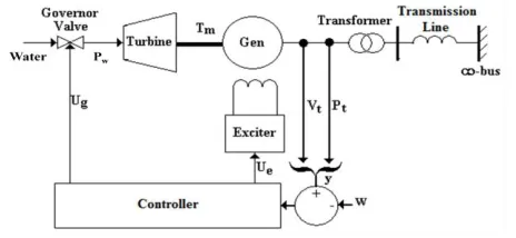
[image:2.612.54.286.585.692.2]

The block diagram of the sample controlled power system is shown in figure 1 that comprises a hydraulic turbine driving a synchronous generator which is connected to an infinite bus via a step-up transformer and a transmission line. The output real power Pt and terminal voltage Vt at the generator terminals are measured and fed to the controller. The outputs of the controller (system control inputs) are fed into the generator-exciter and governor-valve. In the simulation studies described here, the nonlinear equations of the synchronous generator are represented by a third-order nonlinear model based on park’s equations. The hydraulic turbine, governor valve and exciter are each represented by a first order model. The model equations are as follows [12-19]:

Fig. 1 Controlled sample hydropower system

The Mechanical equations

The rotor speed of the generator is given by:

δ (t) = ω(t) (1)

The mechanical equation of the motion is as follows:

H πf0

dω(t)

dt + Dω = Pm− Pt

i.e

Mdω(t)

dt + Dω = Pm− Pt (2)

Where,

M = H

πf0 and f0= ω0 2π

The electrical generator dynamics equations

dEq′(t) dt =

1

T_do′ (Efd t − Eq(t)) (3)

The electrical equations (assumed xd′ = xq)

Eq t = Eq′ t + (xd− xq)Id t (4)

Pt t = Eq t Iq t (5)

Id t =

Eq′ t _Vscos δ(t) x_ds′ (6)

Iq t =

Vssin δ(t) x_ds′ (7) Eq′ t = xadIf(t)(8)

Vt t = Vd t

2

+ Vq t

2 12

(9)

Vd t = Eq′ t − xd′Id t (10) Vq t = xd′Iq t (11)

xds = xd+ xT+ xLxds′ = xd′ + xT+ xLxs = xT+ xL

More details about power system modelling can be seen in [20-23]

Using the above equations, we can express Pt(t) as

Pt t =

Vsxds

x_ds′ 2Eq

′_{t sinδ t}

−(xd− xq) Vs

2

xds′

2 sinδ t cosδ t (12)

(3)

International Journal of Emerging Technology and Advanced Engineering

15

dω t

dt = (Pm−

Vsxds

x_ds′ 2Eq

′_{t sinδ t}

+(xd− xq) Vs

2

x_ds′ 2 sinδ t cosδ t (13)

− Dω t )ω0

2H

In terms of the state variables Eq′ t and Ef t the

equation (3) becomes

dE_q′ t

dt = ω0rfd

xad Efd t +

x_ds x_ds′ T_do′ Eq

′_{t +}(xd−xq)Vs x_ds′ T_do′ (14)

Where,

Tdo′ = xad ω0rfd

The governor valve equation is given by

Pw U_g =

Kv

1+τ_gs (15)

The exciter equation defined by

E_fd U_e =

1

1+τ_es (16)

The turbine equation

Pm P_w =

1

1+τ_bs (17)

In terms of the state variables Efd, Pw and Pm the

equations (15)-(17) written as follow:

Pw dP_w(t)

dt = −P_w

τg + K_v

τgUg (18) dE_fd(t)

dt = −E_fd(t)

τe + 1

τeUe (19) dPm

dt = −Pm

τ_b + 1

τ_bPw (20)

Defining x = [δ δ Eq′ Efd Pw Pm]T the state

variables vector then the equations above can be written in the key form:

x 1= x2

x 2= (x6− K1x3sinx1− K2sinx1cosx1− Dx2)

ω0 2H

x3=

ω0rfd

x_ad x4+ K3x3− K4cosx1

x 4= −x₄

τe + 1 τeUe

x 5= −x5

τg + 1 τgUg

x 6= −x6

τ_b + x5 τ_b

(21)

The output y1, y2 may be expressed in terms of these state variable by

y1= Pt= K1x3sinx1+ K2sinx1cosx1 (22) y2= Vt= Vd2+ Vq2

1

2₍₂₃₎

Where,

Vd= K5sinx1 (24) Vq = K6x3+ K7cosx1 (25) A. Linear model of synchronous generator

A linear Multi-Input Multi-output (MIMO) model of the generator system is required to design a controller for such system. It is derived from the system nonlinear model by linearizing the nonlinear equations (13) and (14) around a specific operating point. The linear state-space model is derived next where the variables shown represent small displacements around the selected operating point.

x t = FXx t + FUu(t)

y(t) = GXx(t) + GUu(t)

(26) Where,

FX =

∂f

∂XT

X ,U =

∂f1

∂X1

⋯ ∂f1

∂Xn

⋮ ⋱ ⋮

∂fn

∂X1

⋯ ∂fn

∂Xn X ,U

FU=

∂f

∂UT

X ,U = ∂f1

∂U1

⋯ ∂f1

∂Um

⋮ ⋱ ⋮

∂fn

∂U1

⋯ ∂fn

∂Un X ,U

GX=

∂g

∂XT

X ,U =

∂g1

∂X1

⋯ ∂g1

∂Xn

⋮ ⋱ ⋮

∂gp

∂X1

⋯ ∂gp

∂Xn X ,U

GU=

∂g ∂UT

X ,U =

∂g₁ ∂U1 ⋯

∂g₁ ∂Um

⋮ ⋱ ⋮

∂gp ∂U1 ⋯

∂gp ∂Um _X_,U

.

FX, FU, GX et GU are the Jacobian matrices of partial

derivatives of f and g respectively to X and U evaluated at the point (X , U).

The linear state-space model defined by

x t = Ax t + Bu(t)

y(t) = Cx(t) + Du(t) (27)

(4)

International Journal of Emerging Technology and Advanced Engineering

16

The matrices A, B, C and D have the form:

A =

0 1 0 0 0 0

K8

−Dω0

2H K9 0 0

ω0 2H

K10 0 K3

ω₀r_fd

xad 0 0

0 0 0 −1

τe 0 0

0 0 0 0 −1

τg 0

0 0 0 0 1

τ_b −1 τ_b

B=

0 0

1 τe 0

0 Kg

τg

0 0

C = K_K11 0 K12 0 0 0

13 0 K14 0 0 0 D =

0 0 0 0

Where

x = [δ δ Eq′ Efd Pw Pm]T State variables vector

u = [Ue Ug]T Control input vector

y = [Pt Vt]T Measurement vector

Pt= K11x1+ K12x3 Output Power Vt= K13x1+ K14x3 Terminal voltage

Expressions for parameters K1, K2, K3, K4, K5, K6, K7,

K8, K9, K10, K11, K12, K13 and K14 in the system model are

given in Appendix

B. State space to transform function conversion

Consider the state equation (27). We may take its Laplace transform and rearrange it as follows:

sX s = AX s + BU(s)→ sI − A X s = BU(s) (28)

If we combine this with the transform of the output equation: Y s = CX s + DU(s), we getY s =

C sI − A −1_{BU s + DU(s)}

Or, equivalently

Y s

U s = C sI − A

−1_{B + D}₍₂₉₎

In the Control Systems Toolbox, the command

num, den = ss2tf(A, B, C, D, i) converts the state equation

to a transfer function for ith input.

III. MULTIVARIABLE LINEAR QUADRATIC GAUSSIAN

CONTROL ALGORITHM

Let us, consider the following m × m process model [24]:

A q−1_{y t = B q}−1_{u t − 1 + C q}−1_{ξ t}₍₃₀₎

Where,

A q−1_{= I}

m+ A1q−1… … … … . . +Anaq−naAjϵRm,m

B q−1_{= B}

0+ B1q−1… … … … . . +Bnbq−nbBjϵRm,m

C q−1_{= C}

0+ C1q−1… … … … . . +Cncq−ncCϵRm,m

y(t)ϵRm_{is the output vector}

u(t)ϵRm_{is the input vector}

ξ t ϵRm_{is a sequence of independent random vectors}

with zero mean value and finite covariance matrix

q−1_{is the backward shift operator such that}_q−1_{f t =} f(t − 1)

To this model, we can associate the companion block state representation in the observable form by:

x t + 1 = A′x t + B′u t + G′ξ t

y(t) = C′x(t) + ξ t (31)

Where:

A′=

−A1 I′ 0′ ⋯ 0′

−A2 0′ ⋱ ⋱ ⋮

⋮ ⋮ ⋱ ⋱ 0′

⋮ ⋮ 0 ⋱ I

−An 0′ ⋯ ⋯ 0′

B′ =

B0

⋮

Bn

G′ =

C1+ A1

⋮

Cn+ An

C′ = Im 0′ … 0′

A′ϵRmn ,mn_,_B′ϵRmn ,m_,_G′ϵRm,m_,_C′ϵRm,mn

x(t)ϵRmn_{is the system state}

n = max⁡(na, nb, nc)

The problem is to found a control vector by state feedback that minimizing the following criterion:

J = limT→∞ Tt=0 y t − y∗(t) TQ y t − y∗(t) +

uTt−1Λu t−1 (32)

Where:

T is the control horizon

y∗_(t)_{is the reference vector sequence}

is a symmetric semi definite positive matrix Q is a symmetric definite positive matrix

The solution is:

Δu t = −Γ t x t − v t + W(t) (33)

Where,

Γ(t)= B′T_{RB′ + Λ}−1_B′T_RA′₍₃₄₎

(5)

International Journal of Emerging Technology and Advanced Engineering

17

v t

= B′ T_RB′_{+ Λ}−1_B′ T_y∗_{t + 1 + A}′_{− B}′_ΓT_y∗_{t + 2}

+ ⋯ + A′_{− B}′_ΓT m_y∗_{t + l + 1}

+ ⋯ (36)

R(t) is the Riccati matrix

Y∗T = y∗ t 0′ … 0′ (37)

Remark

The solution is an explicit form of the state variables. But they are not available. Therefore a state observer is necessary.

The state observer is given by:

x (t)=Hϕe(t − 1) (38)

Where

H =

−A1 ⋯ −An

⋮ ⋰ ⋮

−An ⋯ 0

−B0 ⋯ −Bn

⋮ ⋰ ⋮

−Bn ⋯ 0

−C1 ⋯ −Cn

⋮ ⋰ ⋮

−Cn ⋯ 0

ϕeT t = y t … y t − n + 1 u t … u t − n

+ 1 ξ t … ξ(t − n + 1)

HϵR3mn

ϕeϵR3mn

ξ t = y (t)-C x(t) (39)

IV. SIMULATION AND DISCUSSION

In order to illustrate the behaviour of the above presented multivariable LQG control algorithm, the simulation results of the sample power system are given by using Matlab Toolbox.

Initial condition (operating point) for the non linear system:

x = [0.775 0 1.434 −0.0016 0.8 0.8]T

The hydropower plant model is as follow:

A q−1_{y t = B q}−1_{u t − 1}

Where:

A1= −1.826₀ _−1.540

A2= 1.21₀ _0.76930

A3= −0.3479₀ _−0.12750

A4= 0.03653 0₀ ₀

B0= _−0.078281.367 −0.03534_1.218

B1= −2.107 −0.06115_0.1818 _−0.8947

B2= _−0.12761.043 0.06876_0.1182

B3= −0.1629 _0.02571 −0.01589_0.02204

B4= 0.003059 0₀ ₀

The simulation has been done with respect to the following considerations:

Parameters of the LQG controller

Λ = 5 0

0 5 Q =

1 0

0 1

The reference Yr is chosen as a square wave.

Simulations were carried out to verify the advantages of using multivariable LQG control in this application. The control objective of the sample power plant is to track a reference. The LQG controller parameters are chosen in order to get an acceptable tracking.

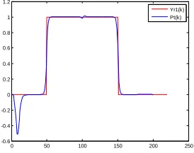
First the non-disturbed sample power system is controlled by multivariable LQG control to track the set point. The tracking response is shown in figure 2, 3, 4 and 5 where we seen that the tracking performance is successfully achieved for both real power Pt and terminal voltage Vt

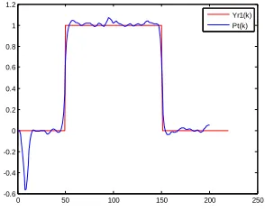
[image:5.612.376.513.510.618.2]

Then, the sample power plant outputs are affected by small random disturbance as shown in figures 6, 7, 8 and 9. It can be seen that the system response follows the reference and the effect of disturbance is well rejected for both real power Pt and terminal voltage Vt

Fig. 2 Power output Pt in noise absence conditions

0 50 100 150 200 250

-0.6 -0.4 -0.2 0 0.2 0.4 0.6 0.8 1 1.2

(6)

International Journal of Emerging Technology and Advanced Engineering

[image:6.612.374.513.128.241.2]

18

[image:6.612.95.243.130.239.2]

Fig. 3 Exciter input Ue in noise absence conditions

Fig. 4 Terminal voltage Vt in noise absence conditions

Fig. 5 Governor Input Ugin noise absence conditions

[image:6.612.375.517.273.389.2]

Fig. 6 Power output Pt in noise presence conditions

Fig. 7 Exciter input Ue in noise presence conditions

[image:6.612.98.244.276.394.2]

Fig. 8 Terminal voltage Vt in noise presence conditions

Fig. 9 Governor Input Ugin noise presence conditions

V. CONCLUSIONS

In this paper, a Multivariable Linear Quadratic Gaussian controller was designed for a sample power system comprising a water turbine driving a synchronous generator. From the simulation results, it is clear that, the LQG control maintains a high level of performances for Pt and Vt responses, in terms of tracking and disturbance

robustness.

APPENDIX

Expressions for parameters K1, K2, K3, K4, K5, K6, K7,

K8, K9, K10, K11, K12, K13 and K14 in the system model are:

0 20 40 60 80 100 120 140 160 180 200 -0.2

-0.15 -0.1 -0.05 0 0.05 0.1 0.15 0.2

0 50 100 150 200 250

-1 0 1 2 3 4 5 6 7 8

Yr2(k) Vt(k)

0 20 40 60 80 100 120 140 160 180 200 -0.8

-0.6 -0.4 -0.2 0 0.2 0.4 0.6 0.8 1 1.2

0 50 100 150 200 250

-0.6 -0.4 -0.2 0 0.2 0.4 0.6 0.8 1 1.2

Yr1(k) Pt(k)

0 20 40 60 80 100 120 140 160 180 200 -0.2

-0.15 -0.1 -0.05 0 0.05 0.1 0.15 0.2

0 50 100 150 200 250

-1 0 1 2 3 4 5 6 7 8

Yr2(k) Vt(k)

0 20 40 60 80 100 120 140 160 180 200 -0.8

[image:6.612.375.513.417.529.2] [image:6.612.105.247.426.540.2] [image:6.612.102.249.574.691.2]

(7)

International Journal of Emerging Technology and Advanced Engineering

19

K1=

Vsxds

x_ds′ 2, K2= −

(x_d−xq)Vs2

x_ds′ 2 , K3= − xds x_ds′ T_do′ ,

K4= −

(x_d−xq)Vs

x_ds′ T_do′ , K5= xqVs

x_ds′ K6= xt +xl

x_ds′

K7=

x_d′Vs x_ds′ ,

K8= −K1x₃₀cos(x_{1 0}) − K2cos(2x_{1 0})

K9= −K1sin(x_{1 0})

K10= −K4sin(x₁₀)

K11= −K1x₃₀cos(x_{1 0}) + K2cos(2x₁₀)

K12 = K1sin(x₁₀)

K13 = ((K5− K72)sin(x_{1 0})cos(x₁₀)

− K6K7x₃₀sin(x₁₀) )((K5sin(x₁₀))2

+ (K6x₃₀+ K7cos(x₁₀))2)

−1 2_K₁₄

= 2K6(K6x₃₀

+ K7cos(x₁₀)) ((K5sin(x₁₀))2

+ (K6x₃₀+ K7cos(x₁₀))2)

−1 2

REFERENCES

[1] Henderson, D. S. September 1998."An advanced electronic load governor for control of Micro hydroelectric power generation", IEEE Transactions Energy Conversion, Vol. 13, No. 3

[2] Henderson,D. S. 1993."Recent Developments of an Electronic Load Governor for Micro Hydroelectric Generation", International Conference on Renewable Energy – Clean Power 2001, pp. 84-88, [3] Working Group on Prime Mover and Energy Supply Models for

System Dynamic Performance Studies,February 1992. Hydraulic turbine and turbine control models for system dynamic studies, Transactions on Power Systems, Vol. 7, NO. 1, pp. 167-179 [4] Vournas,C. D., Papaionnou, G. June 1995. "Modeling and stability

of a hydro plant with two surge tanks", IEEE Trans. Energy Conversion, vol. 10, no. 2, pp. 368-375

[5] Goyal,H., Hanmandlu,M., Kothari,D. P. An Artificial Intelligence based ,Approach for Control of Small Hydro Power Plants, Centre for Energy Studies, Indian Institute of Technology, New Delhi-110016 India

[6] Goyal,H., Bhatti,T. S., Kothari,D. P. 2005."A novel technique proposed for automatic control of small hydro power plants", International Journal of Global Energy Issues, 24 (1/2 ) pp. 29-46 [7] Hydro-thermal System,1988. Proceedings of IEE, Vol. 135, pp.

268-74

[8] Goyal,H., Bhatti,T. S., Kothari,D. P, An Artificial Intelligence based Approach for Control of Small Hydro power plants, Centre for Energy Studies, Indian Institute of Technology, Hauz Khas, New Delhi-110016 (India)

[9] Hanmandlu,M., Goyal,H. 2008. Proposing a new advanced control technique for micro hydro power plants, Electrical power and Energy Systems, pp. 272-282

[10] Zidane, Z., Ait Lafkih, M.,Ramzi, M. 2012. "Simulation Studies of Adaptive Predictive Control for Small Hydro Power Plant", Journal of Mechanical Engineering and Automation, Vol. 2 issue 6, pp. 169-175

[11] Athans, M.,1971. "The role and use of the stochastic Linear-Quadratic-Gaussian problem in control system design". IEEE Transaction on Automatic Control AC-16 (6) pp. 529–552

[12] P. A. W Walker, O. H Abdallah, "Discrete Control of an A.C. Turbo generator by Output Feedback", Proceedings of the IEE, Control & Science, Vol. 125, No. 9,pp. 1031-38, Oct. 1978

[13] Recommended Practice for Excitation System Models for Power System Stability Studies,August, 1992. IEEE Standard,

[14] Aggoune, M. E., Boudjemaa, F., Bensenouci A., et al. 1994. "Design of Variable Structure Voltage Regulator Using Pole Assignment Technique", IEEE Transactions on Automatic Control, Vol. 39, No. 10,pp. 2106-10

[15] Bensenouci, A. Jun 25-28 2002. Variable Structure Control for Voltage/Speed Control in Power System, Proc. 2nd IASTED, Crete, Greece.

[16] Demello, F. P., Concordia,C. 1969. "Concepts of Synchronous Machine Stability as affected by Excitation Control", IEEE Transactions on Power Apparatus and Systems, Vol. 88, No. 4, 316-328

[17] Anderson,P. M., Fouad,A. A. 1993. Power System Control and Stability, IEEE Press

[18] Bensenouci,A.July 2010."Design of a Robust Hi/H2/MOC LMI-based Iterative Multivariable PID for Speed and Voltage Control of a Sample Power System", Journal of Engineering and Computer Sciences, Qassim University, Vol. 3, No. 2, pp. 127-146

[19] Quiroga, D. O.,July 2000. Modelling and nonlinear control of voltage frequency of hydroelectric power plants, doctoral thesis, Universidad Politécnica de Cataluna, Instituto de Organizacion y Control de Sistemas Industriales

[20] AyokuleA., Amuel,I. A., Katende,J., Agbetuyi,A. F. November 2012"Synchronous Generator Excitation Chatter-free Sliding Mode Controller", Asian transactions on Engineering, vol. 02, Issue 05, pp. 57-62

[21] Sedaghati,A. 2006. "A PI Controller Based on Gain-Scheduling for synchronous Generator", Turk J Elec Engin, Vol. 14, No.02, pp.241-250

[22] Tecec,Z., Petrovic,I., Matusko,J. 2010."A Takagi-Sugeno Fuzzy Model of Synchronous Generator Unit for Power Systeme Stabilty Application", AutomaticaVol. 51, Issue 02, pp. 127-137

[23] Agaghi, H., Karrari,M., IEEE, Mahmoodzadeh, A. "Towo New Methods for Synchronous Generator Parameter Estimation" [24] Ait Lafkih, M., 1993. "State observance in adaptive multivariable