Construction noise database (phase 3): Evaluation of established measurement protocol

Evaluation of established measurement 

protocol

Waddington, DC and Moorhouse, AT

Title

Construction noise database (phase 3): Evaluation of established 

measurement protocol

Authors

Waddington, DC and Moorhouse, AT

Type

Monograph

URL

This version is available at: http://usir.salford.ac.uk/490/

Published Date

2006

Construction Noise Database (Phase 3)

Evaluation of Established Measurement Protocol

Report for DEFRA by

Dr. David Waddington

Dr. Andy Moorhouse

April 2006

Contents

1 Executive Summary ... 3

2 Summary ... 4

4 Analytical study... 9

4.1 The point sound source hypothesis ... 9

4.2 Transition points and characteristic ranges ... 10

4.3 Errors due to components within the main source plane ... 11

4.4 Positioning errors within the main source plane ... 14

4.5 Errors due to length of perpendicular to source plane ... 15

4.6 Errors in normalisation to 10m due source-receiver uncertainties ... 17

4.7 Effects of vector wind at short ranges ... 18

5 Experimental study ... 24

5.1 Objectives ... 24

5.2 Overview of experiments ... 24

5.3 Microphone positions and the measurement hemisphere ... 26

5.4 Stationary tests... 28

5.5 Distance tests ... 58

5.6 Dynamic tests ... 64

5.7 Repeatability study from experimental measurements ... 74

6 Discussion ... 77

7 Conclusions ... 79

7.1 Analytical study ... 79

7.2 Experimental study ... 79

3

1 Executive Summary

1.1 The established method for obtaining noise emission data for the update

of a database of noise from construction plant is examined.

1.2 The established measurement protocol involves the collection of plant

noise measurements using a sound level meter, and the normalisation of

the data to 10m.

1.3 The results of analytical and experimental investigations conclude that

this measurement protocol is reasonably accurate and a practical

method for the characterisation of plant sound power on-site for both

2 Summary

2.1 Introduction

2.1.1 An investigation of the accuracy of sound power levels of large

machines as determined from sound pressure level measurements

taken according to the established measurement is presented.

2.2 Analytical study

2.2.1 An analytical study shows that construction plant can be considered to

act as a collection of component point sources after only short

distances. The error in sound power estimation due to approximating

an item of plant of largest dimension 10m by a single point source is

shown to be <1dB.The effect on the L

normalised to 10m is less.

2.2.2 If the entire vehicle is considered to be a finite plane source then the

transition to point source behaviour occurs at ~3m for plant of largest

dimension in excess of 10m.

2.2.3 The single SLM method is sensitive to errors in estimation of the

perpendicular source to receiver distance. For 10% distance

uncertainty this results in a sound power error of ~0.8dB.

2.3 Experimental study

2.3.1 A brief report of the construction machinery noise measurements made

at a limestone quarry in North Wales is given.

2.3.2 Measurements of stationary plant show that the established protocol

using a single SLM at 10m range provides an accurate characterisation

of the L

and of the 1/1 octave spectrum. Levels are within ~1 dB of

values obtained based on the more accurate procedures defined in ISO

374x at all frequencies, except at 250Hz where the level is

underestimated by ~3dB due to the first ground interference dip.

5

2.3.6 The largest cause of variation is source to receiver path, as indicated

by the smaller ±0.4dB 95% confidence limit of the hemisphere method

for the stationary tests.

2.3.7 In practice the sound power determination and normalisation to 10m is

dominated by variations in the running condition of the plant,

determined predominantly by the operator and operation.

2.3.8 These results indicate that the single SLM method at 10m is an

accurate and reliable method for the characterisation of plant sound

power on-site for both stationary and dynamic activities.

3 Introduction

This report presents the results of an analytical and experimental investigation of the

accuracy of sound power levels of large machines as determined from sound pressure level

measurements taken according to the established measurement procedure used in the recent

revision of BS 5228. The methodology of the established measurement protocol is to record

sound pressure levels at a single distance that is considered large compared with the source

dimensions and with the wavelength of sound. These measurements include the estimation of

1/1 octave band and A-weighted sound pressure levels. For plant performing normal

stationary activities these are derived from Leq recordings, while for dynamic plant these are

derived from Lmax recordings made during drive-by. The procedure includes a normalisation to

a 10m distance, based on the assumption that the sound power propagates hemispherically

from a point source located at the geometrical centre of the plant. For large noisy sources

these far field measurements are usually the only practicable method when assessing in situ.

Propagation of noise in the open atmosphere is a complicated statistical problem, since the

atmosphere is in constant fluctuation by its nature. Density in temperature, wind and humidity

are never uniform in a given volume of air under observation, nor are they constant in time.

Sound waves travelling through the atmosphere are affected by these non-uniformities.

However the effects of these factors on sound propagation are not large unless the

transmission path is very long, of the order of hundreds of meters. Usually it can be

approximated that the air is an ideal, homogenous and loss free medium. Further it can be

assumed that all sources are composed of numerous point sources, and that each elemental

point source radiates noise energy incoherently in all directions, neglecting the nature of wave

motion. These assumptions are reasonable and very useful for engineering noise prediction

and control.

The principal objectives of source output quantification are as follows:

i. comparison of sound powers of machines and plant for the purpose of user selection

ii. source labelling

iii. predicting the sound pressure field and associated adverse effects, such as hearing

7 standardised test methods have been developed by the International Organisation for

Standardisation (ISO). In Europe the CEN standards closely follow most ISO standards.

Since the sound pressure level generated by a source varies with distance, direction and

environmental conditions, and the presence of other extraneous sources adds to the sound

produced by a source under test to an unpredictable degree, these methods usually require

the isolation of the source in an acoustical controlled environment. ISO 3745 (3744) requires

an anechoic or semi anechoic test environment. The measurement surface is described

around the source and divided into a number of segments. The sound pressure is sampled at

one point in each segment. It is implicitly assumed that the intensity vector lies normal to the

measurement surface. ISO 3741 (3742-1/2) requires a reverberant environment where the

source sound power is equal to the estimated rate of energy dissipation by the walls,

determined either from an array of fixed microphones distributed over the room volume, or

from a mechanised continuous transverse of the volume. The other ISO 374- standards are

variants on these methods with empirically derived factors to correct for non-ideal conditions.

Noise fall-off with distance has been the subject of earlier work. The fundamental work of

Maekawa (1970) shows the noise reduction along the symmetry axis perpendicular to a

circular and rectangular plane noise source. He also analysed the noise reduction with

distance of plane sound sources composed of small surface elements with different radiation

characteristics. Rathe (1969) derived the sound level along the line perpendicular to the

centre of a rectangular plane noise source. He found the transition distances from plane

source to line source, and from line source to point source behaviour of the rectangular noise

source assuming omni-directional radiation characteristics. This work was expanded upon by

Ellis (1970) concerning receiving points on and outside the boundary of the rectangular sound

source. Janacek (1989) analysed analytical propagation models of plane sound sources, and

together with a numerical integration, derived the intensity for a plane sound source and

compared the results with measurement. The prediction of ground effects caused by sound

radiated from a finite panel was investigated by Li (1989) using a numerical model. The model

assumed omni-directional sound radiation of a panel over an impedance plane, and the sum

pressure caused by each element was computed using a point source ground model above

an impedance boundary. The sound pressure of the panel was evaluated using numerical

integration. The effect of source directivity regarding the ground effects was analysed by

Hohenwater (1990), who reasserted the finding of Rathe that fall-off with distance

perpendicular to a noise radiating surface is like a point source or line source, depending on

the geometric dimensions of the rectangular noise source and the receiver distance.

This topic has also been well researched by authors developing the ISO procedures for

determination of sound power level. Holmer (1977) for example performed an investigation to

place error bounds on several proposed measurement procedures, chiefly through the

comparison with sound power levels determined from far field measurements. The data

analysis centred on the comparison of sound power levels estimated from measured sound

derived for each of several proposed ISO procedures for determination of sound power level.

The near field measurements were found to produce an overestimate of the far field power

level with the magnitude of the overestimate depending on the measurement surface shape.

A recent resurgence in interest has resulted from outdoor Noise Directive 2000/14/EC

concerning the labelling of machines with guaranteed sound power levels. A report by

Jonasson (1999) addressed the determination of emission sound pressure level and sound

power level in situ. An assessment of reproducibility uncertainties for use in international

standards on the determination of power was performed by NPL (2000). An analytical study of

the uncertainties for A weighted sound power level determination using sound pressure

measurements due to end the number of microphones, to the angle error and to the

impedance error for the ISO 3740 series of standards has recently been examined by Loyau

(2006). Carletti (2006) recently presented an inter-laboratory test for the assessment of

reproducibility uncertainties of earth-moving machines. The findings of the above theoretical

work are applied in the following analytical study of the established measurement protocol.

Much of the research that formed the foundation of the ISO procedures for determination of

9

4 Analytical study

4.1 The point sound source hypothesis

The measurement hypothesis is that the plant sound power can be accurately characterised

by a single positioned measurement made over sufficient duration. Further it is asserted that

this sound power can be normalised to a distance of 10m using point source propagation over

a hard plane. This is equivalent to assuming that at the receiving position the plant acts as a

point source propagating over an acoustically hard plane.

We first consider that a piece of large plant can be considered as a collection of point

sources. A real sound source has its own dimensions, but can be treated as a point source

from a receiving point sufficiently distant from the source. The wave front diverges from a

point source and radiates sound energy spherically. Sound intensity decreases inversely with

the square of distance, and this relationship is the well-known inverse square law. When a

sound source is directional the inverse square law is also valid for any one direction.

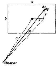
Rathe (1969) showed that for the following geometry of a finite plane source dimensions b>c

that characteristic ranges can be distinguished.

Figure 1: Finite plane source of dimensions b >c from Rathe (1969)

Here the sound source is a rectangular area of dimensions b and c, and the observer is

situated at a distance a on the vertical axis of symmetry of the source. Three characteristic

ranges can be distinguished. The first is near the source where a<<b and a<<c.

The sound pressure equation reduces to:

with W the total power of the source, and zo the characteristic impedance of the medium. This

expression has no dependence on a and so the sound pressure remains constant near the

which corresponds to a line source.

The third range is given by a>>b and a>>c. when

for an attenuation equivalent to that of a point source.

4.2 Transition points and characteristic ranges

The sound pressure level as a function of distance is represented in the figure below.

Figure 2: Sound pressure level attenuation with distance for a finite plane source from

11

Component Height b(m) Length c(m)

Engine 2 2

Exhaust 0.5 0.2

Bucket 1 1

Wheel chains 2 2

Table 1: Face Shovel component sources and dimensions

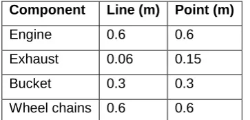
Then the above components approximate to line and point sources at distances given in the

following table.

Component Line (m) Point (m)

Engine 0.6 0.6

Exhaust 0.06 0.15

Bucket 0.3 0.3

Wheel chains 0.6 0.6

Table 2: Transition distances for Face Shovel component sources

These values show that the Face Shovel can be considered as a collection of point sources

from a source to receiver distance greater than 0.6m.

4.3 Errors due to components within the main source plane

Since we considered the vehicle and operations to act as a single point source at a given

distance, it is therefore necessary to estimate the error due to the difference in distance for

each source to receiver. We first consider a source located in the plane of the vehicle at a

x

r

r

SLM

Main source

(engine)

Component source

(bucket)

Figure 3: Plant considered as a main point source and component point source located

at a distance x away in the same vertical plane.

We measure

_L

pand calculate

8

log

20

1



L



r



L

The actual component sound power level

_L

8

log

20

0



L



r



L

If the error in component source estimation is

L

L





L

13

r

r

x

L

log

20







r

x

r

L

1 2 2 1 10

log

10







So as

log

₀

1 2 10



r

x

0



L



Rearranging we can obtain an expression for the ratio of component source distance

_x

main source to receiver distance

_r

1as a function of maximum permissible error in sound

power level estimate.

1

10





Lw

r

x



Taking a sound level meter at a main source to receiver distance of 10m then the maximum

error in sound power level estimation for various component source distances from the main

source can be calculated as shown in table below, and is shown graphically in figure 4.

Max



_L

Ratio

r

x

1

Max

_x

for

_r



10

m

1 0.5 5

0.5 0.35 3.5

0.1 0.15 1.5

Table 3: Limits on component source displacement for given uncertainty for SLM to

main source distance r1=10m

The influence of this error in component level on the LAeq at 10m is numerically smaller than

the values shown in the table. This is because the component sound power level is a smaller

value than the main source and so when combined by decibel arithmetic the error has

sound power level becomes ~0.3B in LAeq at 10m.

4.4 Positioning errors within the main source plane

The expression derived above can be used to estimate the uncertainties in sound power level

due to errors in locating the source within the main source plane. The figure below shows the

error in sound power level against the uncertainty in horizontal source position estimate for

the SLM at 10m perpendicular distance.

0 1 2 3 4 5 6 7 8 9 10

0 0.5 1 1.5 2 2.5 3

Error in source position x (m)

E

rr

o

r

in

L

w

e

s

ti

m

a

te

(

d

B

A

)

Figure 4: Variation in error in Lw measured by SLM at 10m perpendicular source-receiver

15

4.5 Errors due to length of perpendicular to source plane

Now we consider an error y in the length of the perpendicular to the source.

r

SLM

Main source

error y

Figure 5: Plant considered as a point source located at a distance r from the SLM but

with an error y in perpendicular distance.

As above we measure

_L

8

log

20

1



L



r



L

Actually

8

(

log

20

)

10

0



L



r



y



L

Therefore

r

y

r

L





₂₀

_log

10



Rearranging

1

10





Lw

r

y



maximum error in sound power level estimation for errors in the perpendicular source

distance can be calculated as shown in table below.

Max



_L

Ratio

r

y

y

_r



₁₀

_m

1 0.12 1.2

0.5 0.06 0.6

0.1 0.01 0.1

Table 4: Limits on uncertainty in perpendicular source to receiver distance for given

error in sound power level estimate for SLM at 10m

The Lw uncertainty estimates from measurements by a SLM at 10m distance for various

errors in perpendicular source-receiver distance are illustrated in the figure below.

-2 -1 0 1 2 3

E

rr

o

r

in

L

w

e

s

ti

m

a

te

(

d

B

A

17

4.6 Errors in normalisation to 10m due to source-receiver

uncertainties

The above results show that the measurement is far more sensitive to errors in main source

to receiver perpendicular distance than to source displacement within the plane of the main

source. This is likely to have significance when the setting up of recording instruments at a

distance of 10m is found to be impossible for reasons of safety or restricted access. On these

occasions noise measurements are taken at some convenient position and the measured

sound level subsequently adjusted to that for a distance of 10m assuming point source

propagation over a hard plane.

From equation (10), the sound power level calculated from the sound pressure assuming a

10% error in distance estimate is given by:

r

r

r

L

10

log

20







10

1

10

log

20





L



Equally the uncertainty in the sound pressure level assuming a 10% distance estimate

calculated from the sound power level is given by:

10

1

10

log

20





L



Consequently the uncertainty in the sound pressure level normalised to 10m from a sound

pressure level measured at 20m assuming a 10% error in distance is given by:

10

1

10

10

1

10

log

20

2

log

20

2









_





L

dB

L

1

.

66

83

.

1





4.7 Effects of vector wind at short ranges

Experiments were performed to determine the likely uncertainty in the measured sound

pressure level from the SLM at 10m due to variations in the wind vector. A high-power

omni-directional electro-acoustic source with centre height 2m was used to provide a sound power

of 130dB. Acoustical monitoring units with a microphone height of 1.5m were installed with

reference positions near the source. Each station was used as a stand-alone data logger and

audio recorder logging Leq, Lfast and 1/3 octave band spectra each second. The source

emitted pink noise in five-minute sections separated by one-minute sections of silence to

enable background levels to be monitored. Automatic weather stations were used to

simultaneously collect detailed meteorological information. The measurements detailed here

were performed over flat grassland. The correlation of the LAeq with vector wind speed is

illustrated below for a receiver distance 10m. The dotted line shows the sound pressure level

using predicted using the CONCAWE calculation method. The data show a slight correlation

with wind vector, with a downwind enhancement of ~1.5dB clearly evident and some

19

4.7.1 Effect of the ground wave propagation approximation

It is assumed within the method that sound falls off at 6dB per distance doubling. This is the

normal description of propagation from point source over a hard surface. This propagation

model is used initially in the calculation of the sound power of the source when the single

SLM is used to measure at a distance other than 10m. The propagation model is used again

in the normalisation of the sound power measurement to the standardised distance of 10m.

Consequently the choice of propagation model is significant and deserves closer inspection.

A more accurate description would take into account spherical propagation over an

impedance plane, including a description of the ground wave. The figure below illustrates the

predicted sound pressure spectrum for a monitor at a receiver height of 1.5m and distance

10m from a point source of height 2m. Three models had been used for the prediction of

sound pressure. The first is the 6dB per distance doubling for hemispherical propagation from

point source implicit in the established protocol. The second is a plane wave model over an

impedance plane, while the third is a spherical wave model over an impedance plane giving

101 102 103 104 -45

-40 -35 -30 -25 -20 -15

Frequency [Hz]

S

P

L

(d

B

)

re

0

d

B

S

W

L

Ground 10000kR/m Source monitor 10m

Spherical Plane Hemi

Figure 8: Predicted spectrum at 1.5m receiver height of distance 10m from a 2m-height

point source. Three propagation models are: spherical wave model over a hard

impedance plane giving account of the ground wave, plane wave propagation over an

impedance plane, and 6dB per distance doubling for hemispherical propagation from

point source.

The spherical and plane wave models show little difference for this very hard surface.

However the results show the effect of the interference between the direct and ground

reflected source to receiver waves in the form of the ~12dB dip at ~300Hz. In a real

21 An equivalent comparison is performed below for a monitor at 20m distance. As expected due

to the decrease in the path length difference between direct and reflected wave the frequency

of the first interference dip has increased to ~500Hz.

101 102 103 104

-45 -40 -35 -30 -25 -20 -15

Frequency [Hz]

S

P

L

(d

B

)

re

0

d

B

S

W

L

Ground 10000kR/m Source monitor 20m

Spherical Plane Hemi

Figure 9: Predicted spectrum at 1.5m receiver height of distance 20m from a 2m-height

The figure below illustrates predictions performed for reasonably soft grassland. Again the

interference dip is seen to occur at ~300Hz for the spherical and plane wave models, but the

finite impedance of the surface is seen to have an effect in the ground wave resulting in

significant differences between the two spectra.

101 102 103 104

-45 -40 -35 -30 -25 -20 -15

Frequency [Hz]

S

P

L

(d

B

)

re

0

d

B

S

W

L

Ground 100kR/m Source monitor 10m

Spherical Plane Hemi

Figure 10: Predicted spectrum at 1.5m receiver height of distance 10m from a

23 The differences between the plane wave and spherical wave models are seen more clearly in

the following figure showing predictions for a receiver at 20m distance. Here the ground wave

interactions are seen to significantly move the position of the interference dips.

101 102 103 104

-45 -40 -35 -30 -25 -20 -15 Frequency [Hz] S P L (d B ) re 0 d B S W L

Ground 100kR/m Source monitor 20m

Spherical Plane Hemi

Figure 11: Predicted spectrum at 1.5m receiver height of distance 10m from a

2m-height point source over a soft impedance plane.

The computational requirements for the calculations applying the spherical wave model at

multiple frequencies for a combination into 1/3-octave values is considerable and unworkable

under practical circumstances. However, as mentioned above the depth of these interference

dips in a real atmosphere would be significantly reduced due to the effects of turbulence.

Moreover when summed to produce an overall A-weighted sound pressure level the

significance of the dips and peaks will be further reduced. Nevertheless the interference dip is

a real phenomenon that is observed in the measurements using a single SLM at a 10-metre

5 Experimental study

5.1 Objectives

The objectives of the experimental study were:

i. To determine the uncertainties associated with the established protocol for

measurements of sound power when normalised to 10m.

ii. To accurately measure the sound power emitted by a piece of stationary quarry plant

using multiple microphones.

iii. To accurately measure the sound power emitted by a piece of mobile quarry plant

using multiple microphones.

iv. To simultaneously measure the sound pressure levels at 10m or equivalent using a

single SLM.

5.2 Overview of experiments

Consequently three experiments were performed as part of this study. These were:

i. Stationary test, comprising three consecutive measurements of a piece of plant using

multiple microphones and simultaneously the SLM at 10m.

ii. Distance tests, comprising two separate measurements of the fall-off of sound

pressure level with distance from a piece of plant.

iii. Dynamic tests, comprising three independent drive-by measurements using multiple

microphones and simultaneously the SLM at 10m.

The methods and procedures of the acoustical measurements were performed in accordance

with the British Standard 7445. 01dB Symphonie systems were used to log all data. In

addition a 01dB SIP95 sound level meter was used to log data at the nominal single position

of 10m. Due to the need for a drive-by no cables were allowed to cross through the

25 conditions were very wet, such that the quarry road was virtually completely waterlogged. The

wind was easterly with wind speeds typically less than 2m/s with occasional gusts of up to

5m/s. Light snow showers occurred regularly through the day interspersed with the occasional

sunny spell. The low winds, stable temperatures and acoustically hard surface proved ideal

measuring conditions.

The following parameters were logged by each Symphonie. This produced a record of each

operation with time synchronisation between analysers.

i. Short time 1s Leq giving one third octave bands from 20Hz to 20kHz

ii. Short time 1s LAeq to be used for time history

Measurement data are presented to one decimal place and consequently some rounding

errors are evident in the tables below. Audio recordings were also made but not used in the

following analyses.

Filename Description Time Vehicle

Stationary

stationary1 Comparing sound power measurements from

a single SLM at 10m and from 6 mics on a

hemisphere

14h20m05 –

14h21m59

Face Shovel

(wheeled loader)

stationary2 Comparing sound power measurements from

a single SLM at 10m and from 6 mics on a

hemisphere

14h22m00 –

14h23m59

Face Shovel

(wheeled loader)

stationary3 Comparing sound power measurements from

a single SLM at 10m and from 6 mics on a

hemisphere

14h24m00 –

14h25m59

Face Shovel

(wheeled loader)

Dynamic

dynamic1 Drive-by of front loader 14h37m08 –

14h38m25

Front Loader

dynamic2 Drive-by of dumper truck 14h29m15 –

14h30m30

Rigid Dumper

Truck

dynamic3 Drive-by of dumper truck 14h45m29 –

14h47m45

Rigid Dumper

Truck

Distance

distance1 Fall-off with distance from rear of front loader

whilst idling. Distances 10, 20, 30, 40 & 50m.

15h04m16 –

15h07m15

Face Shovel

(wheeled loader)

distance2 Fall-off with distance from side of front loader

performing repeated cycle of simulated

operations. Distances 10, 20, 30, 40, 50 &

15h09m28 –

15h12m32

Face Shovel

Table 5: Summarising measurements used in the following analyses

5.3 Microphone positions and the measurement hemisphere

Measurements were performed on an item of stationary plant positioned in the centre of a

hemisphere of six microphones. The microphones were positioned as detailed in ISO 6393:1998 - Measurement of exterior noise emitted by earth-moving machinery – Stationary

test conditions, p6. The positions are dependent upon the basic length L of the machine. The

relevant distances are summarized in the table below. All construction machinery measured

had a basic length in excess of four metres and so the radius of the hemisphere was 16m.

Length L

(m)

Radius R

(m)

L<1.5 4

1.5<L<4 10

L>4 16

Table 6: Dimensions of hemispherical measurement surface relative to the basic

length of the machine

Mic no x (m) y (m) z (m)

1 2.80 2.80 1.50

2 -2.80 2.80 1.50

3 -2.80 -2.80 1.50

4 2.80 -2.80 1.50

5 -1.08 2.60 2.84

6 -1.08 -2.60 2.84

Table 7: Dimensions of hemispherical measurement surface for basic length of the

27

Mic no x (m) y (m) z (m)

1 11.20 11.20 1.50

2 -11.20 11.20 1.50

3 -11.20 -11.20 1.50

4 11.20 -11.20 1.50

5 -4.32 10.40 11.36

6 -4.32 -10.40 11.36

Table 9: Dimensions of measurement surface for basic length of the machine L<4m

Distances and heights were measured with a tape measure. Allowing for slight variations in

the terrain, tension of the tape measure and reading error, the uncertainty in the distances

and heights was estimated as 0.1m with a 95% level of confidence. Due to the earth barrier on the southeast side of the area, microphone number 1 was repositioned directly south as

shown in the diagram below.

8

6

1

4

3

5

X

N

Figure 12: Schematic of microphone positions. Numbers indicate microphone number.

Bodied Dump Truck is positioned in the centre of hemisphere, the earth barrier is seen in the

south west of the measurement area, and a selection of microphones and the SLM are

labelled.

Figure 13: View of measurement area looking north. The dumper truck is standing at

the centre of the measurement hemisphere.

5.4 Stationary tests

5.4.1 Description of stationary tests

Three stationary tests were performed on the 370kW 50t Face Shovel (wheeled loader). The

face shovel simulated operations with forward driving, reverse driving with reversing warning

alarm, and lifting and lowering of the bucket. A wide range of engine revs was used, and the

29

Figure 14: The Face Shovel during the stationary test

5.4.2 Noise characteristics of stationary tests

The sonogram below shows the general characteristics of the noise generated by the Face

Shovel during the first stationary test. This figure together with the three-dimensional plot

present data averaged over the six microphones of the hemisphere. Virtually all the noise

energy is contained below 2kHz and during intensive operations there is comparatively little

variation with time.

Spectrum at0m 34s 00025 62.04

31.5 63 125 250 500 1k 2k 4k 8k 16k 30.00 90.00

[ID=39] G1 Average over hem ispherical surface0m 34s 000 400 72.86

0m 00s 000 1m 00s 0001m 00s 000 1m 59s 000 31.5 63 125 250 500 1k 2k 4k 8k 16k

Cut at400 Hz 0m 00s 000 74.54

0m 00s 000 1m 00s 0001m 00s 000 1m 59s 000 30.00

90.00

50 70 c1 0m 00s 000 22.4

c2 1m 59s 000 71k

|c2-c1|1m 59s 00070772

30.00 60 90.00

31

Figure 17: Time-varying mean spectrum over 6 mics on hemisphere of radius 16m for

5.4.3 Stationary test 1

5.4.3.1 Amplitude distribution

The comparison of the time-varying sound power levels calculated from measurements from

the six microphones on the hemisphere and from the single SLM at 10m is shown in the plot

below. The levels measured by the SLM at 10m show greater variation than the mean from

six microphones on hemisphere. SWL = hemisphere + 32dBA TUE 28/02/06 14h20m00 115.8 TUE 28/02/06 14h21m59 dB SWL = SLM + 28dBA TUE 28/02/06 14h20m00 115.4 TUE 28/02/06 14h21m59dB

100 105 110 115 120 125 130

20m00 20m30 21m00 21m30 22m00

Figure 18: Comparing time-varying sound power levels calculated from measurements

by single SLM at 10m (blue) and by 6 mics on hemisphere of radius 16m (red) for

stationary test 1

33

SWL = SLM + 28dB Leq 115dBA 5.0 %

0 2 4 6 8 10 12 14 16 18 20 22

100 105 110 115 120 125 130

SWL = hemisphere + 32dB Leq 116dBA 21.6 %

0 2 4 6 8 10 12 14 16 18 20 22

100 105 110 115 120 125 130

Figure 19: Histograms showing the amplitude distribution of one second sound power

levels calculated from one second LAeq measurements at the SLM and from six

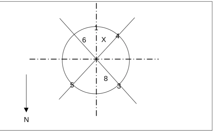
5.4.3.2 Directionality

Directionality is illustrated by the plan view of the stationary test 1 measurement area shown

in the polar plot below. LAw (2min) levels at each of the six microphones on the hemisphere

and the average LAw (2min) level at the sound level meter at radial distance 10m

perpendicular from the centre of the measurement area are compared. These results indicate

that at 16m the Face Shovel is emitting sound reasonably equally over the hemisphere in the

horizontal plane. 0 15 30 45 60 75 90 105 120 135 150 165

180

-165

-150

-135

-120 -105

-90 -75 -60 -45 -30 -15 110dB 115dB 120dB

Mic 6 Mic 1

Mic 4

Mic 5

Mic 8

Mic 3

Figure 20: Polar plot illustrating plan view of stationary test 1 measurement area.

Showing LAw (2min) levels at each of the six microphones on the hemisphere of radius

35 Directionality in the vertical plane is illustrated by the polar cross sectional view of stationary

test 1 measurement looking south. LAw (2min) levels at microphones 3 and 5 at height 1.5m,

6 and 8 at height 11.4m on the hemisphere of radius 16m, and the average LAw (2min) level

at the sound level meter at radial distance 10m perpendicular from the centre of the

measurement area are shown. These results indicate that at 16m the Face Shovel is emitting

sound equally over the hemisphere in the vertical plane.

0 15 30 45 60

75 90

105 120

135

150

165

180

 

110dB 115dB

120dB

Mic 4 Mic 5

Mic 6 Mic 8

Figure 21: Polar plot illustrating cross sectional view of stationary test 1 measurement

looking south. Showing LAw (2min) levels at microphones 3 and 5 at height 1.5m, 6

and 8 at height 11.4m on the hemisphere of radius 16m (red X) and the average LAw

(2min) level at the sound level meter at radial distance 10m perpendicular from the

below. In the first, the average sound power spectra over 2 min calculated from

measurements by the 6 mics on hemisphere for stationary test 1 is compared with the overall

average. The second plot shows the difference sound power spectra between the mean over

hemisphere and each of the 6 mics. Also shown is the overall level difference obtained by a

summation of all frequency differences. These results indicate that of the six microphones,

the position providing poorest agreement with the mean over hemisphere is Mic 5, which is

seen to detect a lower sound power at higher frequencies. This is perhaps an indication that a

barrier effect due to the vehicle body was reducing some bucket noise at this location. The

sound power spectrum measured by Mic 1 gives best agreement with the average over the

hemisphere. Furthermore Mic 1 is the microphone positioned closest to the sound level

meter, indicating that the positioning of the sound level meter was optimal for the

measurement of the sound power spectrum.

[ID=54] Av erage G1 Hemisphere time-av eraged Lw spectrum 100 113.7 1.6 k 109.4

[ID=65] Av erage G2 Mic 6 t ime-av eraged Lw spectrum 100 112.8 1.6 k 109.2

[ID=66] Av erage G1 Mic 3 t ime-av eraged Lw spectrum 100 112.5 1.6 k 105.0

[ID=67] Av erage G2 Mic 8 t ime-av eraged Lw spectrum 100 111.7 1.6 k 106.7

[ID=68] Av erage G1 Mic 4 t ime-av eraged Lw spectrum 100 111.1 1.6 k 108.1

[ID=69] Av erage G1 Mic 5 t ime-av eraged Lw spectrum 100 116.3 1.6 k 110.3

75 80 85 90 95 100 105 110 115 120

A* 115.8

A* 115.3

A* 115.4

A* 115.2

A* 114.9

37 [ID=70] Av erage G1 Hemisphere - Mic 6 time-av eraged Lw spectrum100 0.9 1.6 k 0.1

[ID=71] Av erage G1 Hemisphere - Mic 3 time-av eraged Lw spectrum100 1.2 1.6 k 4.4

[ID=72] Av erage G1 Hemisphere - Mic 8 time-av eraged Lw spectrum100 2.0 1.6 k 2.6

[ID=73] Av erage G1 Hemisphere - Mic 4 time-av eraged Lw spectrum100 2.6 1.6 k 1.2

[ID=74] Av erage G1 Hemisphere - Mic 5 time-av eraged Lw spectrum100 -2.6 1.6 k -1.0

[ID=75] Av erage G1 Hemisphere - Mic 1 time-av eraged Lw spectrum100 -1.6 1.6 k -3.2

-10 -5 0 5 10 15 20

31.5 63 125 250 500 1 k 2 k 4 k 8 k 16 k

A* 12.6

A* 12.1

A* 12.7

A* 12.8

A* 13.4

A* 10.5

A*

Figure 23: Difference in sound power spectra between mean over hemisphere and each

measurement area, showing Lw (2min) 1/1 octave spectra levels at each of the four 1.5m

microphones on the hemisphere, the figure below is seen. These results indicate that the

vehicle is reasonably omni-directional at most frequencies, although some directionality is

seen at 125Hz (red) and at 8kHz (green) at the rear of the vehicle.

0 15 30 45 60 75 90

105 120

135

150

165

180

-165

-150

-135

-120 -105

-90 -75 -60

-45 -30

-15 130dB

140dB 150dB

Figure 24: Polar plot illustrating plan view of stationary test 1 measurement area.

Showing Lw (2min) 1/1 octave spectra levels at each of the four 1.5m microphones on

39 Similarly the figure below shows the polar plot illustrating the cross sectional view of

stationary test 1 measurement looking south. Showing Lw (2min) 1/1 octave spectra levels at

four microphones on the hemisphere, these results indicate that at 16m the Face Shovel is

emitting sound equally over the hemisphere in the vertical plane at most frequencies.

However a 3dB increase is seen at the rear of the vehicle at 125Hz (red).

0 15 30 45 60

75 90

105 120

135

150

165

180

 -15

120dB 130dB

140dB 150dB

Figure 25: Polar plot illustrating cross sectional view of stationary test 1 measurement

looking south. Showing Lw (2min) 1/1 octave spectra levels at four microphones on the

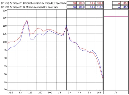
5.4.3.3 Comparison of hemisphere and SLM measurements

The 1/3 octave sound power spectra calculated from measurements by the single SLM at

10m and by 6 mics on hemisphere for stationary test 1 are shown in the figure below. Also

seen is the calculated overall LAW level. The difference between the two spectra is within ~2dB

at most frequencies as illustrated in the figure below, although following the A weighting the

overall levels agrees within ~0.3dB.

[ID=54] Av erage G1 Hemisphere time-av eraged Lw spectrum 100 113.7 1.6 k 109.4

[ID=56] Av erage G1 SLM time-av eraged Lw spect rum 100 113.3 1.6 k 110.6

70 75 80 85 90 95 100 105 110 115 120

31.5 63 125 250 500 1 k 2 k 4 k 8 k 16 k

A* 115.8

A* 115.5

A*

Figure 26: Comparing average sound power spectra calculated from measurements by

41 [ID=48] Av erage G1 SLM - hemisphere time-av eraged Leq spectrum 100 1.6 1.6 k 3.2

-10 -8 -6 -4 -2 0 2 4 6 8 10

31.5 63 125 250 500 1 k 2 k 4 k 8 k 16 k

Figure 27: Difference between average sound power spectra calculated from

measurements by single SLM at 10m and by mean of 6 mics on hemisphere of radius

measurements by the single SLM at 10m and those calculated from the measurements at the

6 mics on hemisphere in the figures below. The normalisation from 16m to 10m was

performed using the point source over a hard plane method.

Hemisphere normalized to 10m 31.5 76.5 16 k 63.8

SLM @ 10m 31.5 73.0 16 k 65.8

60 65 70 75 80 85 90

31.5 63 125 250 500 1 k 2 k 4 k 8 k 16 k

A* 87.9

A* 87.7

A* Figure 28: Comparing 1/1 octave band spl spectra at 10m from measurements by

single SLM at 10m and calculated from measurements at 6 mics on hemisphere of

43 [ID=90] Av erage G1 Hemi - SLM time-av eraged 1/1 oct av e spectra normalized to 10m 250 3.1 2 k -0.8

-10 -8 -6 -4 -2 0 2 4 6 8 10

31.5 63 125 250 500 1 k 2 k 4 k 8 k 16 k

Figure 29: Difference between 1/1 octave band spl spectra at 10m from measurements

by single SLM at 10m and calculated from measurements at 6 mics on hemisphere of

radius 16m for stationary test 1

Frequency

(Hz)

63 125 250 500 1 k 2 k 4 k 8 k 10m Normalised LAeq

(dB)

Hemi 83.3 86.7 84.5 84.3 82.0 82.5 74.1 70.9 87.9

SLM 82.0 85.8 81.4 83.2 81.0 83.4 73.8 71.0 87.7

Hemi-SLM 1.3 0.9 3.1 1.1 1.0 -0.9 0.3 -0.1 0.2

Table 11: Comparing 1/1 octave band spl spectra at 10m from measurements by single

SLM at 10m and calculated from measurements at 6 mics on hemisphere of radius 16m

level spectrum using a single SLM. Levels at most frequencies are within 1 dB except in the

250Hz band where a difference of 3dB is seen, thought to be due to the first interference dip

at the SLM and engine noise. The calculation of the first interference dip between the sound

level meter and at microphones on the hemisphere is summarised in the table below. During

the measurements the SLM was positioned at a range of 10m and height of 1.5m. Four of the

microphones on the hemisphere were positioned at a height of 1.5m and at a range of 16m,

while two of the microphones were positioned at a height of 11.4m and a range of 16m.

SLM @ 10m range

& 1.5m height

Hemi @16m range

& 1.5m height

Hemi @16m range

& 11.4m height

Direct path length (m) 10.6 16.4 17.2

Reflected path length (m) 11.9 17.3 22.9

Path difference (m) 1.3 0.9 5.7

f=c/path difference (Hz) 258 385 60

Table 12: Calculation of first interference dip at the sound level meter and at

45

5.4.4 Stationary test 2

During stationary test 2 the Face Shovel performed slightly more variable operations than

those in stationary test 1. This is evident in the plot below comparing sound power level as

calculated from the measurements by the SLM at 10m and the hemisphere. SWL = Hemi + 32dBA TUE 28/02/06 14h22m00 116.0 TUE 28/02/06 14h23m59 dB SWL = SLM + 28dBA TUE 28/02/06 14h22m00 114.3 TUE 28/02/06 14h23m59dB

90 95 100 105 110 115 120 125 130

22m00 22m30 23m00 23m30 24m00

Figure 30: Comparing time-varying sound power levels calculated from measurements

by single SLM at 10m (blue) and by 6 mics on hemisphere of radius 16m (red) for

stationary test 2

This variation in calculated sound power level is illustrated by the amplitude distribution

histograms shown below. These results show that although the overall levels show excellent

agreement, the SLM measured levels vary more widely than those from the mean of the

hemisphere. These data are summarised in the table below.

Measurement Unit SWL Lmin Lmax StdDev

SWL = hemisphere + 32dBA dBA 116.0 109.3 121.7 2.5

SWL = SLM + 28dBA dBA 114.3 98.7 122.5 5.6

Table 13: Summarising the one second sound power level distributions as measured

0 2 4 6 8 10 12 14 16 18 20

90 95 100 105 110 115 120 125 130

SWL = Hemi + 32dBA Leq 116dBA 19.1 %

47 The 1/3-octave sound power spectra calculated from measurements by the single SLM at

10m and by 6 mics on hemisphere for stationary test 2 are shown in the figure below. Also

seen is the calculated overall LAW level. The difference between the two spectra is again

within ~2dB at most frequencies as illustrated in the figure below, and the A-weighted overall

levels agrees within ~1.0dB.

Hemisphere Time-averaged Lw spectrum 100 113.3 1.6 k 109.1

SLM Time-averaged Lw spectrum 100 112.3 1.6 k 109.0

70 75 80 85 90 95 100 105 110 115 120

31.5 63 125 250 500 1 k 2 k 4 k 8 k 16 k

A* 116.0

A* 115.0

A*

Figure 32: Comparing average sound power spectra calculated from measurements by

Hemi - SLM Lw spectrum 100 -1.1 1.6 k -0.1

-10 -8 -6 -4 -2 0 2 4 6 8 10

31.5 63 125 250 500 1 k 2 k 4 k 8 k 16 k

Figure 33: Difference between average sound power spectra calculated from

measurements by single SLM at 10m and by mean of 6 mics on hemisphere of radius

49 A further comparison is made comparing 1/1 octave band spl spectra at 10m from

measurements by the single SLM at 10m and those calculated from the measurements at the

6 mics on hemisphere in the figures below. The normalisation from 16m to 10m was again

performed using the point source over a hard plane method.

Hemisphere spectrum normalized to 10m 125 86.6 2 k 82.4

SLM spectrum @ 10m 125 85.0 2 k 82.0

60 65 70 75 80 85 90

31.5 63 125 250 500 1 k 2 k 4 k 8 k 16 k

A* 88.1

A* 87.1

A*

Figure 34: Comparing 1/1 octave band spl spectra at 10m from measurements by

single SLM at 10m and calculated from measurements at 6 mics on hemisphere of

[ID=67] Av erage G1 Hemi - SLM 1/1 octav e spectra normalized to 10m 250 2.3 2 k 0.4

-10 -8 -6 -4 -2 0 2 4 6 8 10

31.5 63 125 250 500 1 k 2 k 4 k 8 k 16 k

Figure 35: Difference between 1/1 octave band spl spectra at 10m from measurements

by single SLM at 10m and calculated from measurements at 6 mics on hemisphere of

51 These results again demonstrate the effect of directionality upon the measured sound

pressure level spectrum using a single SLM. Levels at most frequencies are within ~1.5 dB

except in the 250Hz band where a difference of 2.3dB is seen, thought to be due to the first

interference dip at the SLM and engine noise. Despite the more variable sound pressure

levels due to the differing activities of the Face Shovel overall agreement between the SLM

measured LAeq at 10m and the hemisphere LAeq measurements normalised at 10m agree

within 1.0dB.

Frequency

(Hz)

63 125 250 500 1 k 2 k 4 k 8 k 10m Normalised LAeq

(dB)

Hemi 84.4 86.6 85.3 84.5 82.5 82.4 74.3 71.2 88.1

SLM 82.7 85 83 83.3 81.2 82 73.1 70.1 87.1

Hemi-SLM 1.7 1.5 2.3 1.2 1.2 0.4 1.1 1.1 0.4

Table 14: Comparing 1/1 octave band spl spectra at 10m from measurements by single

SLM at 10m and calculated from measurements at 6 mics on hemisphere of radius 16m

5.4.5 Stationary test 3

During stationary test 3 the Face Shovel performed the most variable operations, including a

turn within the hemisphere. This is illustrated in the plot below comparing sound power level

as calculated from the measurements by the SLM at 10m and the hemisphere.

Hemisphere LAeq + 32dB TUE 28/02/06 14h24m00 116.0 28/02/06 14h25m58 dB SLM LAeq + 28dB TUE 28/02/06 14h24m00 114.4 28/02/06 14h25m58dB

80 85 90 95 100 105 110 115 120 125 130 135 140

24m00 24m30 25m00 25m30 26m00

Figure 36: Comparing time-varying sound power levels calculated from measurements

by single SLM at 10m (blue) and by 6 mics on hemisphere of radius 16m (red) for

stationary test 3

The location of the vehicle within the hemisphere varied significantly during this test, on one

occasion approaching the eastern boundary. The SLM measured levels are subsequently

seen to vary more widely than those from the mean of the hemisphere due to greater

53

SLM LAeq + 28dB Leq 114dBA 3.3 %

0 2 4 6 8 10 12 14

80 85 90 95 100 105 110 115 120 125 130 135 140

Hemisphere time-av eraged LAeq + 32dB Leq 116dBA 7.5 %

0 2 4 6 8 10 12 14

80 85 90 95 100 105 110 115 120 125 130 135 140

Figure 37: Histograms showing the amplitude distribution of one second sound power levels

calculated from one second LAeq measurements at the SLM and from six microphones on the

Measurement Unit SWL Lmin Lmax StdDev

SWL = hemisphere + 32dBA dBA 116.2 97.0 130.2 6.9

SWL = SLM + 28dBA dBA 114.4 89.9 128.2 9.0

Table 15: Summarising the one second sound power level distributions as measured

by the SLM and hemisphere during stationary test 3

The 1/3-octave sound power spectra calculated from measurements by the single SLM at

10m and by 6 mics on hemisphere for stationary test 3 are shown in the figure below. Also

seen is the calculated overall LAW level. The difference between the two spectra is greater

than for stationary tests 1 and 2 and is within ~4dB at most frequencies as illustrated in the

figure below. Nevertheless the A-weighted overall levels agree within ~2dB.

Hemisphere 250 108.2 2 k 102.4

SLM 250103.9 2 k 99.9

70 75 80 85 90 95 100 105 110 115 120

31.5 63 125 250 500 1 k 2 k 4 k 8 k 16 k

A* 116.2

A*114.1

A*

55 [ID=64] Av erage G1 Hemi - SLM time-av eraged Lw 1/3 octav e spectrum 250 4.2 2 k 2.5

-10 -8 -6 -4 -2 0 2 4 6 8 10

31.5 63 125 250 500 1 k 2 k 4 k 8 k 16 k

Figure 39: Difference between average sound power spectra calculated from

measurements by single SLM at 10m and by mean of 6 mics on hemisphere of radius

SLM at 10m and those calculated from the measurements at the 6 mics on hemisphere is

shown in the figures below. The normalisation from 16m to 10m was again performed using

the point source over a hard plane method.

Hemisphere normalized to 10m 250 113.0 2 k 109.1

SLM spectrum at 10m 250108.3 2 k107.2

80 85 90 95 100 105 110 115 120

31.5 63 125 250 500 1 k 2 k 4 k 8 k 16 k

A* 116.3

A*114.2

A*

Figure 40: Comparing 1/1 octave band spl spectra at 10m from measurements by

single SLM at 10m (blue) and calculated from measurements at 6 mics on hemisphere

57 [ID=70] Av erage G1 Hemi normalized 10 10m - SLM Hz;(dB[2.000e-05 Pa], PWR) 250 4.7 2 k 1.9

-10 -8 -6 -4 -2 0 2 4 6 8 10

63 125 250 500 1 k 2 k 4 k 8 k

Figure 41: Difference between 1/1 octave band spl spectra at 10m from measurements

by single SLM at 10m and calculated from measurements at 6 mics on hemisphere of

radius 16m for stationary test 3

These results demonstrate the effect of errors in the location of the source to receiver

distance. Levels at most frequencies differ by a more than ~2 dB except in the 250Hz band

where a difference of nearly 5dB is seen, thought to be due to engine noise and the first

interference dip. Despite the more variable sound pressure levels due to the varying location

of the Face Shovel, overall agreement between the SLM measured LAeq at 10m and the

hemisphere LAeq measurements normalised at 10m is 2.1dB.

Frequency

(Hz)

63 125 250 500 1 k 2 k 4 k 8 k 10m Normalised LAeq

(dB)

Hemi 83.9 85.0 85.0 85.7 84.0 81.1 72.0 67.9 88.3

SLM 81.4 81.7 80.3 84.1 81.7 79.2 69.4 64.9 86.2

Hemi-SLM 2.5 3.3 4.7 1.6 2.3 1.9 2.6 3.0 2.1

Table 16: Comparing 1/1 octave band spl spectra at 10m from measurements by single

SLM at 10m and calculated from measurements at 6 mics on hemisphere of radius 16m

5.5 Distance tests

5.5.1 Distance test 1

Tests were performed using the Face Shovel to investigate the variation in sound pressure

level with distance from construction plant under operational conditions. For the first distance

test sound pressure levels were measured on the SIP95 sound level meter at distances of 10,

20, 30, 40 and 50m from the rear of the constantly idling Face Shovel. Each measurement

lasted approximately 15 seconds. Distances were measured by striding out and allowing for

variability in terrain and human error uncertainties are estimated as 10% with a 95% level of confidence. These measurements were repeated three times.

59 The variation in measured LAeq (15s) with distance from the rear of the Face Shovel whilst

ticking over is shown in the figure below. Also shown are spherical propagation curves

calculated from the measurements at 10m and 50m assuming the vehicle is acting as a point

source. It is seen that sound pressure levels fall-off quicker with distance than might be

expected from spherical propagation alone. These differences are perhaps due to near-field

effects, atmospheric absorption, ground absorption, meteorological effects or directionality of

the source, but are most likely due to the undulating topography resulting in a slight barrier

effect.

0 10 20 30 40 50 60

50 55 60 65 70 75 80 85 90 95 100

Distance (m)

L

A

e

q

(

1

5

s

)

Measurement 10m SWL 50m SWL

Figure 43: Showing the variation in measured LAeq (15s) with distance from the rear of

the Face Shovel whilst ticking over. Also shown are spherical propagation curves

calculated from the measurements at 10m and 50m assuming the vehicle is acting as a

These data are presented in the figure below in the form of the variation in sound power level

with distance calculated from the measurements of LAeq (15s). The sound power level is

calculated assuming spherical propagation over a hard plane. It is seen in this case that the

estimated sound power level is lower by approximately 2dBA per distance doubling, thought

to be due to a slight barrier effect as mentioned above.

0 10 20 30 40 50 60

90 95 100 105

Distance (m)

S

W

L

(

d

B

A

)

Figure 44: Showing the variation in sound power level with distance calculated from

measurements of LAeq (15s) from the rear of the Face Shovel whilst ticking over. The

61

5.5.2 Distance tests 2

For the second test sound pressure levels were measured on the SLM at distances of 10, 20,

30, 40, 50 and 60m from the side of the Face Shovel across the open space to the north. The

Face Shovel stood in the centre of the measurement hemisphere and measurements were

simultaneously made on the hemisphere and the SLM. During the measurements at each

distance the vehicle performed a regular and consistent cycle of forward, lift, reverse and

forward movements. Each cycle lasted approximately 15 seconds.

The figure below shows the variation in measured LAeq (30s) with distance. Also shown are

spherical propagation curves calculated from the measurements at 10m and 50m assuming

the vehicle is acting as a point source. It is seen that sound pressure levels fall-off slower with

distance than might be expected from spherical propagation alone. These differences are

perhaps due to near-field effects or directionality of the source, but are more likely due to

variations in the sound power of the source.

0 10 20 30 40 50 60 70 80 90 100

55 60 65 70 75 80 85 90 95 100 105 Distance (m) L A e q ( 3 0 s ) Measurement 10m SWL 60m SWL

Figure 45: Showing the variation in measured LAeq (30s) with distance from the side of

the Face Shovel performing repeated cycles of simulated operations. Also shown are

spherical propagation curves calculated from the measurements at 10m and 50m

with distance calculated from the measurements of LAeq (30s). The sound power level is

calculated assuming spherical propagation over a hard plane. It is seen in this case that the

estimated sound power level increases at a rate of approximately 2dB per distance doubling.

0 10 20 30 40 50 60 70

105 106 107 108 109 110 111 112 113 114 115

Distance (m)

S

W

L

(

d

B

A

)

Figure 46: Showing the variation in sound power level with distance calculated from

measurements of LAeq (30s) from the side of the Face Shovel performing repeated

cycles of simulated operations. The sound power level is calculated assuming