Section Unit Topic Name
Section-1
Introduction to Data Structures
1. Basic concepts, Algorithms, Notations, Data structure operations
2. Implementation of Data Structures, Pseudo code for algorithms
3. Mathematical Notations, Functions and procedure.
Section-2
Arrays
4. Definitions, Index or subscript, Dimensions of an array
5. Memory allocation to array, Memory allocation to one-dimensional array
6. Memory representation of two dimensional arrays 7. Memory representation of Three dimensional
array, memory allocation to multidimensional array
8. Static and dynamic variables, Pointer type variables, Pointers in Pascal
9. Pointers in C, Static and Dynamic memory allocation.
Section-3
Link Lists
10. Dynamic Allocation of memory, Representation of link list, Implementation of link list
11. Insertions of node at Beginning, Insertions of node at end and after specific node.
12. Traversing of entire link list, Concatenation of linked lists, deletion of node from singly link list
13. Merging and reversing of link list
generalized
Section-4
Stack and Queue
15. Implementation of stack, array based stack implementation, Pointer based implementation, application of stacks, applications of stack,
Maze Problem
16. Evaluation Of Expression, Evaluating postfix expression
17. Simulating recursive function using stack ,Passing parameters
18. Return from function, simulation of factorial ,Proving Correctness Of Parentheses In An Expression.
19. Queue implementation, array based, Pointer implementation, Applications of queues, priority queue.
Section-5
Tree and Graphs
20. Tress, n-ary, linked tree representation, binary tree traversal, Searching binary, heap, tree,
avl tree, Threaded trees, splay trees, B-tree
Section-6
Searching And Sorting
21. Linear Search, Binary Search, Tree Searching ,Breadth First Search(BFS), Depth First Search ,General search Trees, Hashing
Section-7
Garbage collection and compaction, Dynamic memory
allocation
22. Reference counting garbage collection, When objects refer to other objects, why reference counting does not work, Mark and sweep garbage collection
23. The fragmentation problem, Stop and copy
collection, the copy algorithm, mark-and-compact garbage collection
24.
Section 1: Introduction to Data Structures
Unit-1. Basic concepts,Algorithms,Notations,Data structure
operations
Introduction
:
Software engineering is the study of ways in which to create large and complex computer applications and that generally involve
many programmers and designers. At the heart of software engineering is with the overall design of the applications and on the creation of
a design that is based on the needs and requirements of end users. While software engineering involves the full life cycle of a software
project, is includes many different components - specification, requirements gathering, design, verification, coding, testing, quality assurance, user acceptance testing, production, and ongoing maintenance.
Having an in-depth understanding on every component of software
engineering is not mandatory, however, it is important to understand that the subject of data structures and algorithms is concerned with
the coding phase. The use of data structures and algorithms is the nuts-and-blots used by programmers to store and manipulate data.
Basics of data structures:
Array : Array is an ordered set which consists of a fixed number of objects. No deletion or insertion operations are performed on arrays.
List : List on the other hand is an ordered set containing of a variable number of elements to which insertions and deletions can be
made. The list is divided into two types : linear list and non linear lists
Algorithms
:
Data Structures: Definition :
The logical inter-relation between elementary data items is
called as data structure. The basic data items include integers, bits, characters. Basically it deals with manipulation and
organization of data, solving problems with computer involves data manipulation. But the data available will usually be in amorphous
form. When different types of such data are related to each other, then we call it to be a data structure.
Ex : Queues, Trees, etc.
D = { d , F , A }
Where,
D : Data structure
d : Domain variable or data objects
A : A set of axioms or rules which governing the operations of these functions on the domain variable.
Advantages:
The major advantages of data structures are :
• It gives different level of organizing data.
• It tells how data can be stored and accessed in its elementary level
Operation on Data Structures:
The operations that can be performed on data structures are :
Creation : This operation creates a data structure. The declaration statement causes space to be created for data upon entering at execution time.
Destroy : This operation destroys the data structure and aids in the efficient use of memory.
Selection : This operation is used to access data within a data structure. The form of selection depends on the type of data structure being accessed.
Update : This operation changes or modifies the data in the data structure and it is an important property in selection operation.
Types of Data Structures:
There are two basic types of data structures:
Linear Data Structure : Stacks, Queues, Linked Lists, etc.
Unit-2.
Implementation of Data Structures, Pseudo code for
algorithms.
Implementation of Data Structures: Operation on Data Structures:
The operations that can be performed on data structures are :
Creation : This operation creates a data structure. The declaration statement causes space to be created for data upon entering at execution time.
Destroy : This operation destroys the data structure and aids in the efficient use of memory.
Selection : This operation is used to access data within a data structure. The form of selection depends on the type of data structure being accessed.
Update : This operation changes or modifies the data in the data structure and it is an important property in selection operation.
Sort: Here we have to arrange data either in ascending or descending order.
There are number of sorting techniques:
Bubble sort Selection sort Insertion sort Merge sort Heap Sort
Pseudo code for algorithms:
An algorithm is a procedure for solving a problem in terms of
the actions to be executed and the order in which those actions are to be executed. An algorithm is merely the sequence of steps taken to
solve a problem. The steps are normally "sequence," "selection, " "iteration," and a case-type statement.
In C, "sequence statements" are imperatives. The "selection" is the "if then else" statement, and the iteration is satisfied by a
Pseudo code is an artificial and informal language that helps programmers develop algorithms. Pseudo code is a "text-based" detail (algorithmic) design tool.
The rules of Pseudo code are reasonably straightforward. All
statements showing "dependency" are to be indented. These include while, do, for, if, switch. Examples below will illustrate this notion.
Examples:
1.If student's grade is greater than or equal to 60 Print "passed"
else
Print "failed"
2. Set total to zero Set grade counter to one
While grade counter is less than or equal to ten
Input the next grade
Add the grade into the total
Set the class average to the total divided by ten
Print the class average.
3.
Initialize total to zero
Initialize counter to zero
Input the first grade
while the user has not as yet entered the sentinel
add this grade into the running total
add one to the grade counter
input the next grade (possibly the sentinel)
if the counter is not equal to zero
set the average to the total divided by the counter
else
UNIT 3: Mathematical Notations, Functions and procedure.
Mathematical Notations:
There are following mathematical notations for time
complexities:
1)Big Oh: It gives asymptotic upper bound of time complexity for given functions
2)Omega: It gives asymptotic lower bound of time complexity for given functions
3)Theta: It gives simultaneously asymptotic lower bound and upper bound of time complexity for given functions
Functions and procedure:
Procedures or functions allow you to group instructions together in one block that can be called from several places in your program. Your code will be more compact, easier to understand and any
modifications can be carried out in a single place. You can use procedures and functions to divide a long and linear block of code into several independent sections.
Procedures accept parameters (also called arguments) and carry
out a task according to these parameters. For example, a procedure can accept a string as a parameter and populate a list with database records for which the content of a given field begins with these
characters.
Functions accept parameters (also called arguments), carry out a
task according to these parameters and return a value of a given type. For example, a function can accept a string as a parameter and
return the first record from a database for which the content of a given field begins with these characters.
You can pass parameters to a function or procedure in two ways : by reference or by value. When a parameter is passed by value, it is
copied into the procedure or function called, and any modification of its value carried out within the procedure or function has no effect on its actual value. When a parameter is passed by reference, any
modification to its value carried out in the procedure or function
Section-2. Array
Unit-4.
Definitions,Index or subscript, Dimensions of an
array
Introduction and Definition:
Simple data types that suit to simple applications. For aggregated data, with same type of element we can use Array.
An array in C / C++ is a collection of related data elements of the same type that are referenced by a common name. Generally, it is
just another data type, aggregate data type.
All the elements of an array occupy a set of contiguous memory
locations and by using an index or subscript we can identify each element.
For example, instead of declaring mark1, mark2, ..., markN to store
and manipulate a set of marks obtained by the students in certain
courses, we could declare a single array variable named mark and use an index, such as j, to refer to each element in mark. This absolutely has simplified our declaration of the variables.
Hence, mark[ j ] would refer to the jth element in the array mark. Thus by changing the value of j, we could refer to any element in the array, so it simplifies our declaration.
For example, if we have 100 list of marks of integer type, we will declare it as follows:
int mark1, mark2, mark3, ..., mark100;
If we have 100 marks to be stored, you can imagine how long we have to write the declaration part by using normal variable declaration?
By using an array, we just declare like this:
int mark[100];
Array definition:
Array is a collection of elements of similar data types which
allocates contiguous memory locations and each element of array is
access with the help of index. Array index is also called as subscript. Array is a collection of homogenous data stored under unique name. The values in an array is called as 'elements of an
array.' These elements are accessed by numbers called as 'subscripts or index numbers.' Arrays may be of any variable type.
Array is also called as 'subscripted variable.'
Syntax: Array declaration Data_Type Array_Name[Size];
Example:
int array[100];
which defines an array named array to hold 100 values of the
primitive type int. If declared within a function, the array dimension may also be a non-constant expression, in which case memory
for the specified number of elements will be allocated. In most contexts in later use, a mention of the variable array is converted
to a pointer to the first item in the array. The sizeof operator is an exception: sizeof array yields the size of the entire array (that
is, 100 times the size of an int). Another exception is the & (address-of) operator, which yields a pointer to the entire array (e.g. int (*ptr_to_array)[100] = &array;).
printf(“%d”,Arr[i]);
here, i= array subscript
Array Dimension: Array can be single,two or multidimensional. Single Dimensional Array is used to represent list.
e.g. int Arr[10];
Two Dimensional Array is used to represent tables of data.
Multidimensional: Multidimensional array can be used store array of two dimensional arrays.
Two Dimensional Array :The array which is used to represent and store
data in a tabular form is called as 'two dimensional array.' Such type of array specially used to represent data in a matrix form.
The following syntax is used to represent two dimensional array.
Syntax:
<data-type> <array_nm> [row_subscript][column-subscript];
Example:
int a[3][3];
In above example, a is an array of type integer which has
storage size of 3 * 3 matrix. The total size would be 3 * 3 * 2 = 18 bytes.
It is also called as 'multidimensional array.'
Unit-4.
Memory allocation to array, Memory allocation to
one-dimensional array.
Memory allocation to array:
Memory to array gets allocated during the time of program compilation. So it is static type of memory allocation technique.
Memory allocation to one-dimensional array: Declaration:
Dimension refers to the array size that is how big the array is. A single dimensional array declaration has the following form:
array_element_data_type array_name[array_size];
Here, array_element_data_type declares the base type of the array, which is the type of each element in the array. array_size defines
how many elements the array will hold. array_name is any valid C / C++ identifier name that obeys the same rule for the identifier naming.
For example, to declare an array of 20 characters, named character, we could use:
char character[20];
Can be depicted as follows:
In this statement, the array character can store up to 20
characters with the first character occupying location character[0] and the last character occupying character[19]. Note that the index runs from 0 to 19. In C / C++, an index always starts from 0 and
ends with (array size-1). So, notice the difference between the array size and subscript/index terms.
Examples of the one-dimensional array declarations:
int x[20], y[50];
float price[10], yield;
The first example declares two arrays named x and y of type int. Array x can store up to 20 integer numbers while y can store up to 50
numbers. The second line declares the array price of type float. It can store up to 10 floating-point values.
The third one declares the array letter of type char. It can store a string up to 69 characters. (Why 69? Remember, a string has a null terminated character (\0) at the end, so we must reserve for it.)
Just like ordinary variables, arrays of the same data type can be declared on the same line. They can also be mixed with ordinary
UNIT 6: Memory representation of two dimensional arrays.
Memory representation of two dimensional array:
We can represent two/multidimensional array through two ways
Row major
Column Major
Some data fit better in a table with several rows and columns.
This can be constructed by using two-dimensional arrays.
A two dimensional array has two subscripts/indexes. The first
subscript refers to the row, and the second, to the column. Its declaration has the following form:
data_type array_name[1st dimension size][2nd dimension size]; For examples:
int x[3][4];
float matrix[20][25];
The first line declares x as an integer array with 3 rows and 4 columns and the second line declares a matrix as a floating-point array with 20 rows and 25 columns.
You can see that for [3][4] 2D array size; the total array size (the total array elements) is equal to 12. Hence:
For n rows and m columns, the total size equal to m*n
The item list is read starting from the first row from left to right, and then goes to the next row and so on.
A set of string s can be stored in a two-dimensional character array with the left index specifying the number of strings and the right index specifying the maximum length of each string.
For example, to store a list of 3 names with a maximum length of 10 characters in each name, we can declare:
// a 2D array that can store 4 names, each is 10 characters long
char name[4][10];
Just like the one-dimensional array, a two dimensional array can also be initialized. For example, the previous first array declaration can be rewritten along with initial assignments in any of the
following ways:
Unit-7.
Memory representation of Three dimensional array,
memory allocation to multidimensional array.
Memory representation of Three dimensional:
UNIT 8: Static and dynamic variables, Pointer type
variables,Pointers in Pascal.
Static and dynamic variables:
A variable to which memory is allocated during the time of program compilation, such variables are called as static variables.
e.g. int x,y,z;
int arr[100];
A variable to which memory is allocated during the time of program execusion, such variables are called as dynamic variables.
e.g. int *x;
x=(int*) malloc(sizeof(int));
Pointer In Pascal :
program pointers1( output );
type int_pointer = ^integer;
var iptr : int_pointer;
begin
new( iptr );
iptr^ := 10;
writeln('the value is ', iptr^);
dispose( iptr )
end.
Pointer type variables:
Variables declared using pointer is called pointer type variable.
int *ptr,x=22;
Unit-9.
Pointers
in
C,
Static
and
Dynamic
memory
allocation.
Pointers in C:
Pointer is a variable which holds address of another variable. So in c programming we declare pointer variable to store address of another variables.
Syntax:
Data_Type * Variable_name;
Example:
int *ptr;
So here ptr is a pointer which contains address of integer variable.
Static Memory Allocation:
Static memory gets allocated to particular variable during the time of program compilation. Once memory is allocated it can not get modified. That's why it is called as static memory allocation.
Dynamic Memory Allocation:
Dynamic memory gets allocated to particular variable during the time of program execution. After memory is allocated to any variable it can be modified as per the requirements. That's why it is called as static memory allocation.
Dynamic memory allocation is one of the three ways of using memory provided by the C/C++ standard. To accomplish this in C the malloc function is used and the new keyword is used for C++. Both of them perform an allocation of a contiguous block of memory, malloc taking the size as parameter:
int *data = new int;
int *data = (int*) malloc(sizeof(int)); //notice the use of sizeof for portability
This memory block can be used whenever needed during the program execution or until explicitly deallocating it, unlike the automatic memory which is available only inside the function or block of instructions where it was declared. Allowing a program to allocate dynamic storage every time it needs more until the program stops can cause it eventually to run out of available space. To prevent this behavior C++ provides the delete operator with the job of recycling a segment of memory allocated with new:
The C function for memory deallocation is free() and has the same behavior as delete, it frees the space pointed by data for future use:
Section-3. Linked lists
Unit-10.
Dynamic Allocation of memory, Representation of
link list, Implementation of link list.
Dynamic Allocation of memory:
As we begin doing dynamic memory allocation, we'll begin to see (if we haven't seen it already) what pointers can really be good for.
Many of the pointer examples in the previous chapter (those which
used pointers to access arrays) didn't do all that much for us that we couldn't have done using arrays. However, when we begin doing dynamic memory allocation, pointers are the only way to go, because
what malloc returns is a pointer to the memory it gives us. (Due to the equivalence between pointers and arrays, though, we will still be
able to think of dynamically allocated regions of storage as if they were arrays, and even to use array-like subscripting notation on them.)
You have to be careful with dynamic memory allocation. malloc
operates at a pretty ``low level''; you will often find yourself having to do a certain amount of work to manage the memory it gives you. If you don't keep accurate track of the memory which malloc has
given you, and the pointers of yours which point to it, it's all too easy to accidentally use a pointer which points ``nowhere'', with
generally unpleasant results. (The basic problem is that if you assign a value to the location pointed to by a pointer:
*p = 0;
and if the pointer p points ``nowhere'', well actually it can be construed to point somewhere, just not where you wanted it to, and
that ``somewhere'' is where the 0 gets written. If the ``somewhere'' is memory which is in use by some other part of your program, or even
worse, if the operating system has not protected itself from you and ``somewhere'' is in fact in use by the operating system, things could get ugly.)
int *ip = malloc(100 * sizeof(int)); if(ip == NULL)
{
printf("out of memory\n");
To allocate dynamic memory we have to use malloc function.
We can deallocate memory using free function.
Representation of link list:
We can represent link list with the help of pointers. To allocate
dynamic memory to node using malloc and go on connecting one node to another node. It will give us link list.
We can use
singly
Doubly
Circular link list
Implementation of link list
:
To implement singly link list we have to performed number of operations like create,display,insert,delete.
To represent node in singly link list we have to write following structure.
struct node
int data;
struct node *next;
}*header=NULL;
void Display()
{
struct node *q;
if(header == NULL)
{
printf("\n\n\t List is empty");
}
else
{
q=header;
printf("\n\n\t Link list is : ");
while(q!=NULL)
{
printf("%d ",q->data);
q=q->next;
}
}
}
struct node* Create()
{
int n,i;
struct node *p,*q;
header=NULL;
scanf("%d",&n);
for(i=0;i<n;i++)
{
p = (struct node*)malloc(sizeof(struct node));
printf("\n\n\t Enter data : ");
scanf("%d",&p->data);
p->next = NULL;
if(header==NULL)
{
header = p;
q=p;
}
else
{
q->next=p;
q=q->next;
}
}
return header;
Unit-11.
Insertions of node at Beginning,Insertions of node
at end and after specific node.
Insertions of node at Beginning:
void Insert_At_Start()
{
struct node *p;
p=(struct node*)malloc(sizeof(struct node));
printf("\n\n\t Enter data : ");
scanf("%d",&(p->data));
p->next=header;
header=p;
printf("\n\n\t %d node is inserted in the link list successfully",p->data);
}
Insertions of node after specific node in singly link list
: To insert a new node after the specified node, first we get the number of the node in an existing list after which the new node is tobe inserted. This is based on the assumption that the nodes of the list are numbered serially from 1 to n. The list is then traversed to
get a pointer to the node, whose number is given. If this pointer is x, then the link field of the new node is made to point to the node
Say suppose new created node is p and q is pointing to the node after which we have to attach new created node. Then,
q->next=p;
p->next=q->next
Insertions of node at the end in singly link list:
To insert node at the last in link list we have to find last node of link list and then attach new created node after that last node.
void Insert_At_Last()
{
struct node *p,*q;
p=(struct node*)malloc(sizeof(struct node));
printf("\n\n\t Enter data : ");
scanf("%d",&p->data);
p->next=NULL;
if(header == NULL)
{
header=p;
}
{
q=header;
while(q->next!=NULL)
{
q = q->next;
}
q->next=p;
printf("\n\n\t %d node is inserted in the link list successfully",p->data);
}
Unit-12.
Traversing of entire link list, deletion of node
from singly link list,Concatenation of linked lists.
Traversing of entire link list:
Traversing link list means visiting each node of link list and displaying its data. To traverse link list we have to do following thing:
void Traverse( struct node *p )
{
printf("The data values in the list are\n");
while (p!= NULL)
{
printf("%d\t",p-> data);
p = p-> link;
}
}
Deletion of node of specific node in singly link list:
Program
# include <stdio.h>
# include <stdlib.h>
struct node *delet ( struct node *, int );
int length ( struct node * );
struct node
{
int data;
struct node *link;
};
struct node *insert(struct node *p, int n)
{
struct node *temp;
if(p==NULL)
{
p=(struct node *)malloc(sizeof(struct node));
if(p==NULL)
{
printf("Error\n");
}
p-> data = n;
p-> link = NULL;
}
else
{
temp = p;
while (temp-> link != NULL)
temp = temp-> link;
temp-> link = (struct node *)malloc(sizeof(struct node));
if(temp -> link == NULL)
{
printf("Error\n");
exit(0);
}
temp = temp-> link;
temp-> data = n;
temp-> link = NULL;
}
return (p);
}
void printlist ( struct node *p )
{
printf("The data values in the list are\n");
while (p!= NULL)
{
printf("%d\t",p-> data);
p = p-> link;
}
void main()
{
int n;
int x;
struct node *start = NULL;
printf("Enter the nodes to be created \n");
scanf("%d",&n);
while ( n- > 0 )
{
printf( "Enter the data values to be placed in a node\n");
scanf("%d",&x);
start = insert ( start, x );
}
printf(" The list before deletion id\n");
printlist ( start );
printf("% \n Enter the node no \n");
scanf ( " %d",&n);
start = delet (start , n );
printf(" The list after deletion is\n");
printlist ( start );
}
/* a function to delete the specified node*/
struct node *delet ( struct node *p, int node_no )
{
struct node *prev, *curr ;
int i;
{
printf("There is no node to be deleted \n");
}
else
{
if ( node_no > length (p))
{
printf("Error\n");
}
else
{
prev = NULL;
curr = p;
i = 1 ;
while ( i < node_no )
{
prev = curr;
curr = curr-> link;
i = i+1;
}
if ( prev == NULL )
{
p = curr -> link;
free ( curr );
}
else
{
prev -> link = curr -> link ;
free ( curr );
}
}
return(p);
}
/* a function to compute the length of a linked list */
int length ( struct node *p )
{
int count = 0 ;
while ( p != NULL )
{
count++;
p = p->link;
}
return ( count ) ;
}
Concatenation of Link list:
Concatenation of two link list means just attaching one link list at the end of another liklists.
Say suppose there are two link lists, Head1 is pointing to first link list and Head2 is pointing to second link list.
So we will write
Node* Concat(Node Head1,Node Head2)
{
Node *p;
p=Head1;
while(p->next!=NULL)
{
p=p->next;
}
p->next=Head2;
return Head1;
Unit-13.
Merging and reversing of link list
Sorting of singly Link list:To sort a linked list, first we traverse the list searching for
the node with a minimum data value. Then we remove that node and append it to another list which is initially empty. We repeat this
process with the remaining list until the list becomes empty, and at the end, we return a pointer to the beginning of the list to which all the nodes are moved, as shown in Figure 20.1.
Reversing a link list:
To reverse a list, we maintain a pointer each to the previous and the next node, then we make the link field of the current node point to the previous, make the previous equal to the current, and the current equal to the next, as shown in Figure 20.2
Prev = NULL;
While (curr != NULL)
{
Next = curr->link;
Curr -> link = prev;
Prev = curr;
Curr = next;
Merging of two link lists:
Merging of two sorted lists involves traversing the given lists and comparing the data values stored in the nodes in the process of traversing.
If p and q are the pointers to the sorted lists to be merged, then we compare the data value stored in the first node of the list pointed to by p with the data value stored in the first node of the list pointed to by q. And, if the data value in the first node of the list pointed to by p is less than the data value in the first node of the list pointed to by q, make the first node of the resultant/merged list to be the first node of the list pointed to by p, and advance the pointer p to make it point to the next node in the same list.
If the data value in the first node of the list pointed to by p is greater than the data value in the first node of the list pointed to by q, make the first node of the resultant/merged list to be the first node of the list pointed to by q, and advance the pointer q to make it point to the next node in the same list.
Repeat this procedure until either p or q becomes NULL. When one of the two lists becomes empty, append the remaining nodes in the non-empty list to the resultant list.
Program to merge two link lists: # include <stdio.h>
# include <stdlib.h>
struct node
{
int data;
struct node *link;
};
struct node *merge (struct node *, struct node *);
struct node *insert(struct node *p, int n)
{
struct node *temp;
if(p==NULL)
{
p=(struct node *)malloc(sizeof(struct node));
if(p==NULL)
printf("Error\n");
exit(0);
}
p-> data = n;
p-> link = NULL;
}
else
{
temp = p;
while (temp-> link!= NULL)
temp = temp-> link;
temp-> link = (struct node *)malloc(sizeof(struct node));
if(temp -> link == NULL)
{
printf("Error\n");
exit(0);
}
temp = temp-> link;
temp-> data = n;
temp-> link = NULL;
}
return (p);
}
void printlist ( struct node *p )
{
printf("The data values in the list are\n");
while (p!= NULL)
{
printf("%d\t",p-> data);
p = p-> link;
}
}
struct node *sortlist(struct node *p)
{
struct node *temp1,*temp2,*min,*prev,*q;
q = NULL;
while(p != NULL)
{
prev = NULL;
min = temp1 = p;
temp2 = p -> link;
while ( temp2 != NULL )
{
if(min -> data > temp2 -> data)
{
min = temp2;
prev = temp1;
}
temp1 = temp2;
temp2 = temp2-> link;
}
if(prev == NULL)
p = min -> link;
else
prev -> link = min -> link;
min -> link = NULL;
if( q == NULL)
q = min; /* moves the node with lowest data value in the list
pointed to by p to the list pointed to by q as a first node*/
else
{
temp1 = q;
/* traverses the list pointed to by q to get pointer to its
last node */
while( temp1 -> link != NULL)
temp1 -> link = min; /* moves the node with lowest data value
in the list pointed to
by p to the list pointed to by q at the end of list pointed by
q*/
}
}
return (q);
}
void main()
{
int n;
int x;
struct node *start1 = NULL ;
struct node *start2 = NULL;
struct node *start3 = NULL;
/* The following code creates and sorts the first list */
printf("Enter the number of nodes in the first list \n");
scanf("%d",&n);
while ( n-- > 0 )
{
printf( "Enter the data value to be placed in a node\n");
scanf("%d",&x);
start1 = insert ( start1,x);
}
printf("The first list is\n");
printlist ( start1);
start1 = sortlist(start1);
printf("The sorted list1 is\n");
printlist ( start1 );
/* the following creates and sorts the second list*/
printf("Enter the number of nodes in the second list \n");
scanf("%d",&n);
{
printf( "Enter the data value to be placed in a node\n");
scanf("%d",&x);
start2 = insert ( start2,x);
}
printf("The second list is\n");
printlist ( start2);
start2 = sortlist(start2);
printf("The sorted list2 is\n");
printlist ( start2 );
start3 = merge(start1,start2);
printf("The merged list is\n");
printlist ( start3);
}
/* A function to merge two sorted lists */
struct node *merge (struct node *p, struct node *q)
{
struct node *r=NULL,*temp;
if (p == NULL)
r = q;
else
if(q == NULL)
r = p;
else
{
if (p->data < q->data )
{
r = p;
temp = p;
p = p->link;
temp->link = NULL;
}
{
r = q;
temp =q;
q =q->link;
temp->link = NULL;
}
while((p!= NULL) && (q != NULL))
{
if (p->data < q->data)
{
temp->link =p;
p = p->link;
temp =temp->link;
temp->link =NULL;
}
else
{
temp->link =q;
q = q->link;
temp =temp->link;
temp->link =NULL;
}
}
if (p!= NULL)
temp->link = p;
if (q != NULL)
temp->link = q;
}
return( r) ;
Unit-14. Applications of link list – Doubly, circular and
generalized.
Applications of Link lists:
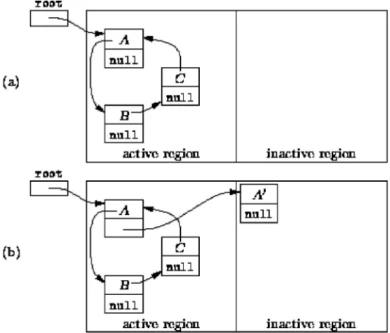
1)A doubly linked list is used to maintain both the list of allocated blocks and the list of free blocks by the memory manager of the operating system. To keep track of the allocated and free portions of memory, the memory manager is required to maintain a linked list of allocated and free segments. Each node of this list contains a starting address, size, and status of the segment. This list is kept sorted by the starting address field to facilitate the updating, because when a process terminates, the memory segment allocated to it becomes free, and so if any of the segments are freed, then they can be merged with the adjacent segment, if the adjacent segment is already free. This requires traversal of the list both ways to find out whether any of the adjacent segments are free. So this list is required to be maintained as a doubly linked list. For example, at a particular point in time, the list may be as shown in Figure 20.21.
2)Generalized link list is used to represent polynomial of any term and evaluate arithmetic expressions.
3)A linked list is suitable for representation of sparse matrices. 4)Linked lists can be used for manipulation of symbolic
Section-4. Stack and Queue
Unit-15.
Implementation
of
stack,
array
based
stack
implementation,Pointer based implementation, application of
stacks, applications of stack,Maze Problem .
Definition :
Lists permit the insertion or deletion of an element to occur
only at one end. A linear list belonging to this subclass is called a stack. They are also referred to as push down lists.
The insertion operation is referred to as PUSH and the deletion operation as POP. The most accessible element in a stack is known as the TOP of the stack.
Since insertion and deletion operations are performed at one end of
stack, the elements can only be removed in the opposite order from that in which they were added to the stack. Such a linear list is frequently referred to as a LIFO ( Last-In First-Out ) LIST.
An example of stack is the “in” tray of a busy executive. The files pile up in the tray and whenever the executive has time to clear the
files, he/she takes it off from the top. That is, files are added at the top and removed from the top. Therefore stacks are sometimes referred to as LIFO structure.
Fig. Stack A pointer TOP
A pointer TOP keeps track of the top element in the stack. Initially when the stack is empty, TOP has a value of –1 and when the stack
contains a single element, TOP has a value of 0 ( Zero ) and so on. Each time a new element is inserted in the stack, the pointer is
incremented by 1. The pointer decrements by 1 each time a deletion is made from the stack.
STACK STRUCTURE D = { d , F , A }
d : Array or a node (structure)
d = { a , TOP }
Here, a : Simple array or structure
TOP : Index or Pointer
F : PUSH, POP, DISPLAY, MODIFY
A : EMPTY, OVERFLOW, UNDERFLOW
Implementation of stack:
Stack can be implemented by two ways:
- Array
- Link lists
ALGORITHM : STACK
Procedure PUSH(S,TOP,X) :
This procedure inserts an element X to the top of the stack which is represented by a vector S consisting MAX elements with a
pointer TOP denoting the top element in the stack.
STEP 1 : [Check for stack underflow]
If (TOP>=max-1)
then write(stack overflow)
Return
STEP 2 : [Increment TOP]
TOP <-- TOP+1
STEP 3 : [Insert element]
S[TOP] <-- X
STEP 4 : [Finished]
Return
The first step of this algorithm checks for an overflow condition. If such a condition exists, then the insertion can't be performed and an
Procedure POP(S,TOP,X) : This procedure removes top element from the stack.
STEP 1 : [Check for the underflow on stack]
If (TOP<0)
then write(stack underflow)
Return
STEP 2 : [Hold the former top element of stack into X]
X <-- S[TOP]
STEP 3 : [Decrement the TOP pointer or index by 1]
TOP <-- TOP-1
STEP 4 : [finished-Return the popped item from the stack]
Return(X)
As Underflow condition is checked for in the first step of the
algorithm. If such a condition exists, then the deletion cannot be performed and an appropriate error message results.
Procedure Display(S,TOP) : This procedure displays the contents of the stack i.e., vector S.
STEP 1 : [check for empty on stack]
if (TOP==-1)
then write('stack empty')
Return
STEP 2 : [Repeat through STEP 3 from i=TOP to 0]
Repeat through STEP 3 for i=TOP to 0 STEP-1]
STEP 3 : [Display the stack content]
write (S[i])
STEP 4 : [Finished]
The first step of this algorithm checks for an empty condition. If such a condition exists, then the contents of the stack cannot be displayed and an appropriate error message results.
Linked list
The linked-list implementation is equally simple and straightforward. In fact, a simple singly-linked list is sufficient to implement a
stack -- it only requires that the head node or element can be
removed, or popped, and a node can only be inserted by becoming the
new head node.
Unlike the array implementation, our structure typedef corresponds
not to the entire stack structure, but to a single node:
typedef struct stack { int data;
struct stack *next;
} STACK;
Such a node is identical to a typical singly-linked list node, at
least to those that are implemented in C.
The push() operation both initializes an empty stack, and adds a new
node to a non-empty one. It works by receiving a data value to push
onto the stack, along with a target stack, creating a new node by
allocating memory for it, and then inserting it into a linked list as
the new head:
void push(STACK **head, int value) {
STACK *node = malloc(sizeof(STACK)); /* create a new node */
if (node == NULL){
fputs("Error: no space available for node\n", stderr); abort();
} else { /* initialize node */
node->data = value;
node->next = empty(*head) ? NULL : *head; /* insert new head if any */
*head = node; }
}
A pop() operation removes the head from the linked list, and assigns
the pointer to the head to the previous second node. It checks
whether the list is empty before popping from it:
int pop(STACK **head)
{
fputs("Error: stack underflow\n", stderr); abort();
} else { /* pop a node */ STACK *top = *head;
int value = top->data; *head = top->next; free(top);
return value; }
}
Applications of Stack:
Stack is used for following purposes-
1)To evaluate arithmetic expressions from- infix to postfix, infix to prefix and vice versa
2)To evaluate arithmetic expressions- prefix, postfix
3)To remove recursion stack is used
4)To traverse any graph DFS non recursively.
Maze Problem:
This is one of the classical problems of computer science. There is a rat trapped in a maze. There are multiple paths in the maze from the starting point to the ending point. There is some cheese at the exit. The rat starts from the entrance of the maze and wants to get to the cheese. This problem can be attacked as follows. Have a m*m matrix which represents the maze.For the sake of simplifying the implementation, have a boundary around your matrix and fill it up with all ones. This is so that you know when the rat is trying to go out of the boundary of the maze. In the real world, the rat would know not to go out of the maze, but hey! So, initially the matrix (I mean, the maze) would be something like (the ones represent the
The rat can move in four directions at any point in time (well, right, left, up, down). Please note that the rat can't move
diagonally. Imagine a real maze and not a matrix. In matrix language
Moving right means adding {0,1} to the current coordinates. Moving left means adding {0,-1} to the current coordinates. Moving up means adding {-1,0} to the current coordinates. Moving right means adding {1,0} to the current coordinates.
The rat can start off at the first row and the first column as the entrance point.
From there, it tries to move to a cell which is currently free. A cell is free if it has a zero in it.
It tries all the 4 options one-by-one, till it finds an empty cell. If it finds one, it moves to that cell and marks it with a 1 (saying it has visited it once). Then it continues to move ahead from that cell to other cells.
If at a particular cell, it runs out of all the 4 options (that is it can’t move either right, left, up or down), then it needs to
backtrack. It backtracks till a point where it can move ahead and be closer to the exit.
If it reaches the exit point, it gets the cheese, ofcourse. The complexity is O(m*m).
Here is some pseudocode to chew upon
findpath() { Position offset[4]; Offset[0].row=0; offset[0].col=1;//right; Offset[1].row=1; offset[1].col=0;//down; Offset[2].row=0; offset[2].col=-1;//left; Offset[3].row=-1; offset[3].col=0;//up;
// Initialize wall of obstacles around the maze for(int i=0; i < m+1;i++)
maze[0][i] = maze[m+1][i]=1; maze[i][0] = maze[i][m+1]=1;
Position here; Here.row=1; Here.col=1;
maze[1][1]=1; int option = 0; int lastoption = 3;
while(here.row!=m || here.col!=m) {
while (option <= LastOption) {
r=here.row + offset[position].row; c=here.col + offset[option].col; if(maze[r][c]==0)break;
option++; }
//Was a neighbor found? if(option <= LastOption) {
path->Add(here);
here.row=r;here.col=c; maze[r][c]=1;
option=0; }
else {
if(path->Empty())return(False); Position next;
Path->Delete(next); If(new.row==here.row)
Option=2+next.col - here.col;
Else { option = 3 + next.row - here.col;} Here=next;
}
return(TRUE); }
Unit-16. Evaluation Of Expression, Evaluating postfix
expression.
Evaluating Prefix Expressions:
Algorithm : Evaluate prefix expression
Input : *+125
Output : 15
Step 1 : Start.
Step 2 : Read prefix string from right to left one
character at a time still the string not ends.
Step 3 : If character is operand then push it on the stack.
Step 4 : If character is operator then
a) Pop two operands from stack i.e operand1 and operand2
b) Evaluate expression or calculate expression.
c) Store result on the stack.
Step 5 : if string is ended then pop the result.
display result and goto step 6.
otherwise go to step2 and continue operation.
Step 6 : Stop
Evaluate Postfix expressions:
Algorithm : Evaluate Postfix Expression.
Input : Postfix string i.e 24+54++
Output : Solution or calculation of expression
based on their values and operators.
result : 15
Steps 1 : start
Steps 2 : Read single character from postfix string
from left to right.(one character at a time)
Steps 3 : If character read is operand or data then
push that character to stack which you
Steps 4 : If element is operator i.e +,-,* etc.
a) pop two operands from stack.
[ Note : pop one operand in case of
single or unary operator like NOT
operator.]
b) evaluate expression form by these two.
operands and operator.
c) Push result of expressioin on the stack.
Steps 5 : if no more characters in the postfix string
then pop stack and display result
if there is more character then repeat
steps from step2 to step5.
Steps 6 : stop
One of the most useful characteristics of a postfix expression is that the value of such an expression can be computed easily with the aid of a stack of values. The components of a postfix expression are processed from left to right as follows:
1.If the next component of the expression is an operand, the value of the component is pushed onto the stack.
2.If the next component of the expression is an operator, then its operands are in the stack. The required number of operands are popped from the stack; the specified operation is performed; and the result is pushed back onto the stack.
After all the components of the expression have been processed in this fashion, the stack will contain a single result which is the
final value of the expression. Figure - illustrates the use of a stack to evaluate the RPN expression given in Equation
Figure: Evaluating the RPN Expression in Equation using a Stack
Unit-17.
Simulating recursive function using stack, Passing
parameters.
Program: Stack Application--A Single-Digit, RPN Calculator
Notice that the RPNCalculator function is passed a reference to a Stack object. Consequently, the function manipulates the stack entirely through the abstract interface. The calculator does not depend on the stack implementation used! For example, if we wish to use a stack implemented using an array, we would declare a StackAsArray variable and invoke the calculator as follows:
On the other hand, if we decided to use the pointer-based stack implementation, we would write:
StackAsLinkedList s; RPNCalculator (s);
The running time of the RPNCalculator function depends upon the number of symbols, operators and operands, in the expression being evaluated. If there are n symbols, the body of the for loop is executed n times. It should be fairly obvious that the amount of work done per symbol is constant, regardless of the type of symbol encountered. This is the case for both the StackAsArray and theStackAsLinkedList stack implementations. Therefore, the total running time needed to evaluate an expression comprised of n symbols is O(n).
Simulation for recursive function using stack:
With the ideas illustrated so far, we can implement any iterative process by specifying a register machine that has a register corresponding to each state variable of the process. The machine repeatedly executes a controller loop, changing the contents of the registers, until some termination condition is satisfied. At each point in the controller sequence, the state of the machine (representing the state of the iterative process) is completely determined by the contents of the registers (the values of the state variables).
Implementing recursive processes, however, requires an additional mechanism. Consider the following recursive method for computing factorials, which we first examined in section :
(define (factorial n) (if (= n 1)
1
(* (factorial (- n 1)) n)))
As we see from the procedure, computing n! requires computing (n-1)!. Our GCD machine, modeled on the procedure
(define (gcd a b) (if (= b 0) a
(gcd b (remainder a b))))
In the case of factorial (or any recursive process) the answer to the new factorial subproblem is not the answer to the original problem. The value obtained for (n-1)! must be multiplied by n to get the final answer. If we try to imitate the GCD design, and solve the factorial subproblem by decrementing the n register and rerunning the factorial machine, we will no longer have available the old value of n by which to multiply the result. We thus need a second factorial machine to work on the subproblem. This second factorial computation itself has a factorial subproblem, which requires a third factorial machine, and so on. Since each factorial machine contains another factorial machine within it, the total machine contains an infinite nest of similar machines and hence cannot be constructed from a fixed, finite number of parts.
Nevertheless, we can implement the factorial process as a register machine if we can arrange to use the same components for each nested instance of the machine. Specifically, the machine that computes n! should use the same components to work on the subproblem of computing (n-1)!, on the subproblem for (n-2)!, and so on. This is plausible because, although the factorial process dictates that an unbounded number of copies of the same machine are needed to perform a computation, only one of these copies needs to be active at any given time. When the machine encounters a recursive subproblem, it can suspend work on the main problem, reuse the same physical parts to work on the subproblem, then continue the suspended computation.
In the subproblem, the contents of the registers will be different than they were in the main problem. (In this case the n register is decremented.) In order to be able to continue the suspended computation, the machine must save the contents of any registers that will be needed after the subproblem is solved so that these can be restored to continue the suspended computation. In the case of factorial, we will save the old value of n, to be restored when we are finished computing the factorial of the decremented n register.
Since there is no a priori limit on the depth of nested recursive calls, we may need to save an arbitrary number of register values. These values must be restored in the reverse of the order in which they were saved, since in a nest of recursions the last subproblem to be entered is the first to be finished. This dictates the use of a stack, or ``last in, first out'' data structure, to save register values. We can extend the register-machine language to include a stack by adding two kinds of instructions: Values are placed on the stack using a save instruction and restored from the stack using a restore instruction. After a sequence of values has been saved on the stack, a sequence of restores will retrieve these values in reverse order.
controller cannot simply loop back to the beginning, as with an iterative process, because after solving the (n-1)! subproblem the machine must still multiply the result by n. The controller must suspend its computation of n!, solve the (n-1)! subproblem, then continue its computation of n!. This view of the factorial computation suggests the use of the subroutine mechanism described in section , which has the controller use a continue register to transfer to the part of the sequence that solves a subproblem and then continue where it left off on the main problem. We can thus make a factorial subroutine that returns to the entry point stored in the continue register. Around each subroutine call, we save and restore continue just as we do the n register, since each ``level'' of the factorial computation will use the same continue register. That is, the factorial subroutine must put a new value in continue when it calls itself for a subproblem, but it will need the old value in order to return to the place that called it to solve a subproblem.
Figure shows the data paths and controller for a machine that implements the recursive factorial procedure. The machine has a stack and three registers, called n, val, and continue. To simplify the data-path diagram, we have not named the register-assignment buttons, only the stack-operation buttons (sc and sn to save registers, rc and rn to restore registers). To operate the machine, we put in register n the number whose factorial we wish to compute and start the machine. When the machine reaches fact-done, the computation is finished and the answer will be found in the val register. In the controller sequence, n and continue are saved before each recursive call and restored upon return from the call. Returning from a call is accomplished by branching to the location stored in continue. Continue is initialized when the machine starts so that the last return will go to fact-done. The val register, which holds the result of the factorial computation, is not saved before the recursive call, because the old contents of val is not useful after the subroutine returns. Only the new value, which is the value produced by the subcomputation, is needed.
Unit-18.
Return
from
function,
simulation
of
factorial,Proving
Correctness
Of
Parentheses
In
An
Expression.
Passing parameters to Recursive procedures: Factorial:
A classic example of a recursive procedure is the function used to calculate the factorial of a natural number:
Pseudocode (recursive):
function factorial is:
input: integer n such that n >= 0
output: [n × (n-1) × (n-2) × … × 1]
1. if n is 0, return 1
2. otherwise, return [ n × factorial(n-1) ]
end factorial
The function can also be written as a recurrence relation:
bn = nbn − 1
b0 = 1
This evaluation of the recurrence relation demonstrates the computation that would be performed in evaluating the pseudocode above:
Computing the recurrence relation for n = 4:
b4 = 4 * b3
= 4 * 3 * b2
= 4 * 3 * 2 * b1
= 4 * 3 * 2 * 1 * 1
= 4 * 3 * 2 * 1
= 4 * 3 * 2
= 4 * 6
= 24
This factorial function can also be described without using recursion by making use of the typical looping constructs found in imperative
programming languages:
Pseudocode (iterative):
function factorial is:
input: integer n such that n >= 0
output: [n × (n-1) × (n-2) × … × 1]
1. create new variable called running_total with a value of 1
2. begin loop
1. if n is 0, exit loop
2. set running_total to (running_total × n)
3. decrement n
4. repeat loop
3. return running_total
end factorial
The imperative code above is equivalent to this mathematical definition using an accumulator variable t:
The definition above translates straightforwardly to functional programming languages such as Scheme; this is an example of iteration
Parentheses
C allows you to override the normal effects of precedence and associativity by the use of parentheses as the examples have
illustrated. In Old C, the parentheses had no further meaning, and in
particular did not guarantee anything about the order of evaluation in expressions like these:
int a, b, c;
a+b+c;
(a+b)+c;
a+(b+c);You used to need to use explicit temporary variables to get a
particular order of evaluation—something that matters if you know that there are risks of overflow in a particular expression, but by forcing the evaluation to be in a certain order you can avoid it.
Standard C says that evaluation must be done in the order indicated
by the precedence and grouping of the expression, unless the compiler can tell that the result will not be affected by any regrouping it might do for optimization reasons.
So, the expression a = 10+a+b+5; cannot be rewritten by the compiler
as a = 15+a+b; unless it can be guaranteed that the resulting value of a will be the same for all combinations of initial values of a and b. That would be true if the variables were both unsigned integral
types, or if they were signed integral types but in that particular implementation overflow did not cause a run-time exception and
UNIT-19:
Queue
implementation,array
based,Pointer
implementation, Applications of queues, priority queue.
FIFO is an acronym for First In, First Out, an abstraction in ways of organizing and manipulation of data relative to time and
prioritization. This expression describes the principle of aqueue processing technique or servicing conflicting demands by ordering process by first-come, first-served (FCFS) behaviour: what
comes in first is handled first, what comes in next waits until the first is finished, etc.
Thus it is analogous to the behaviour of persons standing in line, where the persons leave the queue in the order they arrive, or
waiting one's turn at a traffic control signal. FCFS is also the shorthand name (see Jargon and acronym) for the FIFO operating system
scheduling algorithm, which gives every process CPU time in the order they come. In the broader sense, the abstraction LIFO, or Last-In-First-Out is the opposite of the abstraction FIFO organization, the
difference perhaps is clearest with considering the less commonly
used synonym of LIFO, FILO—meaning First-In-Last-Out. In essence, both are specific cases of a more generalized list (which could be accessed anywhere). The difference is not in the list (data), but in
the rules for accessing the content. One sub-type adds to one end, and takes off from the other, its opposite takes and puts things only on one end.[1]
A priority queue is a variation on the queue which does not qualify
for the name FIFO, because it is not accurately descriptive of that data structure's behavior. Queueing theoryencompasses the more general concept of queue, as well as interactions between strict-FIFO
queues.
Example C language code using array
This c language example uses a fixed length array and global
variables for conceptual simplicity. An array is inefficient because of time spent copying items to the front of the queue, but is simple to code compared to creating a linked list.
// global data structure for simplicity
#define QMAX 100
int Q [QMAX];
int qLast = 0;
int debug = TRUE;
void printqueue()
{
printf ("queue: ");
for (int i = 0; i < qLast; i++){
printf ("%i ", Q[i]);
}
printf ("\n");
}
void enqueue(int qItem)
{
Q[qLast] = qItem;
qLast++;
if (debug){
printf("enqueue %d\n", qItem);
printqueue();
}
}
int dequeue()
{
/* head of queue is always 0 */
int qReturn = Q[0];
/* move items moves up by one towards head */
for (int i = 0; i < qLast - 1; i++){
Q[i] = Q[i + 1];
}
qLast--;
if (debug){
printf("dequeue %d\n", qReturn);
printqueue();
}
return qReturn;
}
Queue implementation:
struct fifo_node
{
struct fifo_node *next;
value_type value;
};
clas