Freaque waves during Typhoon Krosa

Ann. Geophys., 27, 2633–2642, 2009 www.ann-geophys.net/27/2633/2009/

© Author(s) 2009. This work is distributed under the Creative Commons Attribution 3.0 License.

Annales

Geophysicae

Freaque waves during Typhoon Krosa

P. C. Liu1, H. S. Chen2, D.-J. Doong3, C. C. Kao4, and Y.-J. G. Hsu5 1_{NOAA Great Lakes Environmental Research Laboratory, Ann Arbor, MI, USA} 2_{NOAA National Centers for Environmental Prediction, Camp Spring, MD, USA} 3_{National Taiwan Ocean University, Keelung, Taiwan}

4_{National Cheng Kung University, Tainan, Taiwan}

5_{Marine Meteorology Center, Central Weather Bureau, Taipei, Taiwan}

Received: 21 May 2008 – Revised: 27 May 2009 – Accepted: 24 June 2009 – Published: 1 July 2009

Abstract. This paper presents a subjective search for North Sea Draupner-like freaque waves from wave measurement data available in the northeastern coastal waters of Taiwan during Typhoon Krosa, October 2007. Not knowing what to expect, we found rather astonishingly that there were more Draupner-like freaque wave types during the build-up of the storm than we ever anticipated. As the conventional ap-proach of defining freaque waves as Hmax/Hs>2 is inef-fective to discern all the conspicuous cases we found, we also tentatively proposed two new indices based on differ-ent empirical wave grouping approaches which hopefully can be used for further development of effective indexing toward identifying freaque waves objectively.

Keywords. Meteorology and atmospheric dynamics (Ocean-atmosphere interactions; Waves and tides) – Oceanography: physical (surface waves and tides)

1 Introduction

The word “freaque” in freaque waves was initially used in-tentionally as a portmanteau word to encompass the common synonymously used expressions of “freak” or “rogue” waves. As neither freak nor rogue waves have been clearly defined, it is only vaguely implying some kind of unexpected, larger than usual waves. In this paper we choose to affix to the word freaque with two additional implications: first, it is a kind of steep elevated abnormal wave which may be resem-bles the Draupner type waves to be discussed later, and sec-ond, freaque waves are not analogous to the extreme waves, because a freaque wave may be a local extreme, but most extreme waves are not at all freaque waves.

Correspondence to: P. C. Liu

([email protected])

The term “freak” waves was first recognized by Draper (1964) nearly four and one-half decades ago. Later on the word “rogue” waves have also being used alternately. But it has only been in more recent years that the concept of freak or rogue waves had become widely accepted academically and also become common usage in the media for the pos-sible cause of a plethora of relevant, semi-relevant, or even irrelevant wave events. For the ocean wave studies, however, freaque waves remain under-explored beyond a number of theoretical as well as empirical conjectures. While reviews of the current state of physical mechanisms on freaque waves can be found in Dysthe et al. (2008), or Kharif and Peli-novsky (2003) among others, we are still not really knowing where, when, why, and how freaque waves occur in nature. As in many severe storms where freaque waves may be impli-cated, no actual measurement has ever been available other than at most some on site witness speculations.

In one of the most tragic shipping disasters, the loss of the bulk carrier MV Derbyshire during Typhoon Orchid in 9 September 1980 in Western Pacific south of Japan, all hands (42 crew and two wives) on board perished. There were two official investigations into the possible cause. Perhaps Faulkner (2000) summarized the findings of all those inves-tigations best by his postulate that “a steep elevated abnor-mal wave probably collapsed the forward hatch covers dur-ing Typhoon Orchid.” As one of the appointed assessors who examined all possible loss scenarios along with available un-derwater survey of the wreckage and laboratory experiments, Faulkner’s finding is certainly irrefutable. As we alluded ear-lier that we have regarded the description of “steep elevated abnormal” to be justifiably used in defining freaque waves. The postulate of the cause of a steep abnormal wave, how-ever, while entirely conceivable will remain to be a specula-tive conjecture unless actual measurement or veracious evi-dence can be manifested.

2634 P. C. Liu et al.: Freaque waves during Typhoon Krosa

Figures

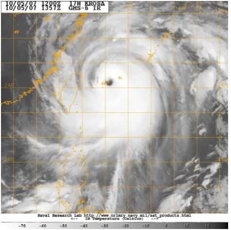
Figure 1. Typhoon Krosa approaching Taiwan. Fig. 1. Typhoon Krosa approaching Taiwan.

during a gale storm in eastern Lake Superior on 10 November 1975 with 29 crew members onboard (NTSB, 1978); and the wreck of the semi-submersible, offshore rig Ocean Ranger during a storm linked to a major Atlantic cyclone while drilling in the Grand Banks area on the North American ctinental shelf on 15 February 1982 with 84 crew members on-board (Royal Commission, 1984). In both cases they seemed to have happened suddenly, there were no survivors, and thus there is speculation that they were overwhelmed by the force of a freaque wave.

Are there freaque waves during a hurricane, typhoon, or severe storm? The answer is clearly affirmative. Guedes Soares et al. (2003) studied storm waves in the North Sea and also in the Gulf of Mexico during the 1969 Hurricane Camille (Guedes Soares et al., 2004). They pioneered the ef-forts of examining freaque waves from wave measurements under large storms. Presumably their findings can be applica-ble to the North Sea storms and the tropical storms in Atlantic and Pacific alike. The availability of wave data has not been plentiful. During the 2004 Hurricane Ivan, there were 11 Na-tional Data Buoy Center (NDBC) buoys in the Gulf of Mex-ico recording standard-deviation wave heights, Hs, among other meteorological parameters but NDBC buoys do not provide time-series measurements. Panchang and Li (2006) studied those NDBC data in the Gulf of Mexico during Ivan and arguing for the importance of evaluation of statistics of extremely high waves under hurricane conditions. That’s separate from studying actual freaque waves. Sea going ships seldom ventured out there during a typhoon or hurricane, hence wave measurements usually can not be readily vali-dated through ship observations such as those VOS reports

Figure 2. The track of Typhoon Krosa. The colored circles show the strength and location of the typhoon center. The number inside represents the date of occurrence. (Color code: Magenta : Extratropical Cyclone; Blue : Tropical Depression; Green : Tropical Storm; Yellow : Severe Tropical Storm; Red : Typhoon.)

Fig. 2. The track of Typhoon Krosa. The colored circles show the strength and location of the typhoon center. The number inside rep-resents the date of occurrence (color code: Magenta: Extratropical Cyclone; Blue: Tropical Depression; Green: Tropical Storm; Yel-low: Severe Tropical Storm; Red: Typhoon).

presented in Gulev et al. (2003). In this paper we expect to answer the afore mentioned question by using wave measure-ments made recently from a buoy deployed in the northeast-ern coastal waters of Taiwan during Typhoon Krosa in Octo-ber 2007. As the hourly data covered only a few days during the typhoon build up, they can only be leading to local-time incidences, not sufficient to make general climatological in-ferences.

2 The Typhoon Krosa

In the early October 2007, a tropical depression that origi-nated east of the Philippines in the Western Pacific Ocean, rapidly intensified to become Typhoon Krosa.

It was later upgraded to a Category 4-equivalent super typhoon as it advanced northwestward toward Taiwan. Its track momentarily hovered and made a small loop back out to sea over the northeastern coastal waters of Taiwan be-fore making landfall on 6 October 2007 (Fig. 1). There were several moored buoys deployed around Taiwan where wave conditions during Krosa were summarily recorded. In particular, the buoy located at longitude 121◦₅₅0₃₀00_{E and}

latitude 24◦₅₀0₅₇00_{N in 38 m water depth recorded a very}

large trough to crest maximum wave height of 32.3 m, which could be the highest knownHmaxever recorded (Liu et al.

2008). The buoy was located near the small Gueishantao Is-land (Fig. 5), 12 km offshore of the northeast coast town of Suao, which was located close to the center of the path of Krosa.

P. C. Liu et al.: Freaque waves during Typhoon Krosa 2635

Figure 3. Representing central pressure, in hPa, of the track shown in Figure 2 as plotted with respect of corresponding date/time with the same color code. Fig. 3. Representing central pressure, in hPa, of the track shown in

Fig. 2 as plotted with respect of corresponding date/time with the same color code.

summary/wnp/s/200715.html.en. It is shown that Krosa fol-lowed a fairly steady northwestern path toward northeast Tai-wan, while the central pressure deepened as wind intensity gradually strengthened to 70 m/s (140 kt) just before making landfall on 6 October 2007.

3 The wave measurement

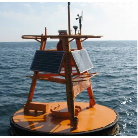
The Central Weather Bureau (CWB) of Taiwan has been constantly developing, deploying, and maintaining moored 2.5 m circular discus hull foam buoys (Fig. 4) in the coastal waters around Taiwan Island for meteorological and ma-rine measurements including ocean wave measurement since 1997. The buoys were designed for reliable operations, with wave following characteristics, and are lightweight for con-venient and safe land and sea transportability. Currently there are nine buoys in operation, all are equipped with heave, pitch, and roll accelerometers sampled at 2 Hz frequency for 10 min duration each hour. In this paper we are concentrat-ing on the one buoy located at longitude 121◦5503000E, and latitude 24◦5005700N in 38 m water depth in the lee of the small offshore Gueishantao Island (Fig. 5). The buoy is lo-cated 12 km offshore of the northeast coast of Taiwan, which was closest to the center path of Typhoon Krosa prior to its landfall. The wave conditions during the onward move-ment of Krosa at this buoy location, as represented by the ocean surface fluctuations inferred from the recorded heave displacements, are used in this paper in search of possible occurrences of freaque waves during the passage of the ty-phoon.

4 The portrait of a freaque wave

What are freaque waves and how do we identify them? These are questions that still lack unified, clear-cut answers. Cur-rently, information is limited to descriptions of the waves at

Figure 4. A deployed CWB Buoy.

Figure 5. The buoy location near Gueishantao off the northeast coast of Taiwan.

Fig. 4. A deployed CWB buoy.

Figure 4. A deployed CWB Buoy.

Figure 5. The buoy location near Gueishantao off the northeast coast of Taiwan.

Fig. 5. The buoy location near Gueishantao off the northeast coast of Taiwan.

2636 P. C. Liu et al.: Freaque waves during Typhoon Krosa

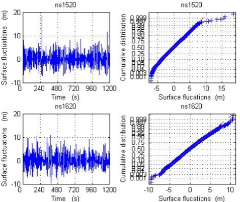
Figure 6. Two wave data recorded on January 1, 1995 at Draupner platform. The upper left panel is considered to be the standard portrait of a freaque wave. Fig. 6. Two wave data recorded on 1 January 1995 at Draupner

plat-form. The upper left panel is considered to be the standard portrait of a freaque wave.

Gorm field (Sand et al., 1990) and Draupner platform (Haver, 2004) were both discovered from conventional wave mea-surements. The wave profile from the Draupner platform, as shown in the upper left panel of Fig. 6, has been widely recognized and generally identified as the exemplary depic-tion of a freaque wave. Since it is also generally construed that freaque waves can happen any time and in any part of the world’s oceans, there must be more Gorm/Draupner-like freaque waves being recorded but that simply have not been discovered or noticed.

The time series plot of the ocean surface fluctuation shown in the upper left panel of Fig. 6 is widely considered as the portrait of a freaque wave, known as the Draupner freaque wave. We see that it clearly does not fit the conventional conceptualization that expects the ocean surface as a Gaus-sian random process. This is shown by the discord in the cumulative distribution between the Gaussian process and the Draupner data on the upper right panel of Fig. 6, espe-cially at the high end. In contrast, measurement at the same sensor one hour later, as shown in the two bottom panels, displays a more customary time series plot and a nearly ac-cordant Gaussian cumulative distribution.

As the discovery and recognition of the Draupner freaque wave time series shown above was basically through visual means, other generally objective approaches of recognizing freaque waves have also been employed. One frequently used approach is to examine the ratioHmax/Hs, the maxi-mum wave height,Hmaxin the time series to the significant

wave height,Hs, which we feel should be more appropri-ately called the standard deviation wave height since it is given by 4*standard deviation in the data. For the Gaussian random process, the zero-upcrossing or zero-downcrossing

Figure 7. Time history of wave heights during Typhoon Krosa. For the three digit numbers on the abscissa, the first number is the day of October and the next two digits give the corresponding

hour. The red vertical bars denote where freaque waves might have occurred.

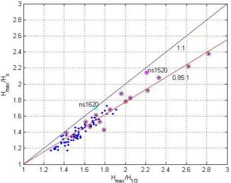
Figure 8. Correlation of the ratios of Hmax/Hs with Hmax/H1/3. The blue line represents the 1:1

perfect fit. The red line is a best eyeball fit, 0.85:1 in this case. The points with a red circle around are the visually picked freaque wave cases.

Fig. 7. Time history of wave heights during Typhoon Krosa. For the three digit numbers on the abscissa, the first number is the day of October and the next two digits give the corresponding hour. The red vertical bars denote where freaque waves might have occurred.

wave heights usually follow a Rayleigh distribution where statisticallyHmaxshould be at most twice theHs, thus it is frequently thought that cases withHmax/Hs>2 are freaque waves. This is what Dysthe et al. (2008) now called the “pragmatic” approach.

One of the well-known equations that correlatesHmax/Hs with the number of zero-upcrossing or zero-downcrossing waves needed in the data for it to occur is

Hmax/Hs= [ln(N )/2]1/2 (1)

whereN is the number of waves encountered in the data. Another minor approach that has only been used for ref-erence purposes is to check into the kurtosis of the data set. The kurtosis for a perfect Gaussian process is 3. Larger kur-tosis values signify a greater departure from Gaussian. As shown in Fig. 6, the Draupner freaque wave has a kurtosis of 4.0648, but an hour later, without the freaque wave, the kurtosis is 3.2842.

5 In search of freaque waves during Krosa

We started by visually examining the wave time series data recorded at Gueishantao buoy during the build up of Typhoon Krosa prior to landfall on Taiwan, 3–6 October 2007. We looked at each data set during this period for Draupner-like cases and are rather astonished to have found more cases than we ever expected. As shown in Fig. 7, the vertical red bars denote the cases that were visually recognized as possibly Draupner-like freaque waves. The detailed plotting of each time series and the corresponding test of Gaussian probabil-ity distribution, similar to Fig. 6, are given in the Appendix.

P. C. Liu et al.: Freaque waves during Typhoon Krosa 2637 Figure 7. Time history of wave heights during Typhoon Krosa. For the three digit numbers on

the abscissa, the first number is the day of October and the next two digits give the corresponding hour. The red vertical bars denote where freaque waves might have occurred.

Figure 8. Correlation of the ratios of Hmax/Hs with Hmax/H1/3. The blue line represents the 1:1

perfect fit. The red line is a best eyeball fit, 0.85:1 in this case. The points with a red circle around are the visually picked freaque wave cases.

Fig. 8. Correlation of the ratios ofHmax/HswithHmax/H1/3. The blue line represents the 1:1 perfect fit. The red line is a best eyeball fit, 0.85:1 in this case. The points with a red circle around are the visually picked freaque wave cases.

Draupner case. They are, in our visualization, at least poten-tial freaque wave cases. As shown in the next section with a few exceptions, their kurtosis and their departure from Gaus-sian distribution tend to sustain our visual choice. Clearly visual picks tend to find more cases than the conventional in-dicators. But who is in position to quibble which one really is or is not a true freaque wave when we don’t even have a tangible definition for it yet?

6 Circumscribing freaque wave cases

We proceed next to examine conventional approaches to cir-cumscribe freaque waves. As alluded earlier the widely used approach is the use of the ratio of maximum wave height to significant wave height in a given time series wave data. Based on the assumption of Gaussian and Rayleigh distribu-tion theories, a ratio larger than 2 is generally regarded as possibly a freaque wave case. However, some ambiguity is implicated with this approach. One is that the size of time series data has never been specified. Different time length of data invariably leads to different results. The other is that the significant wave height, usually defined as the average of the highest one third wave heights in the data, has been mostly represented by four times the standard deviation in the data – again a result of the assumption of Gaussian and Rayleigh distributions. The significant wave height,H1/3,

and the standard deviation wave height,Hs, are not always the same as we see in Fig. 8 here. The North Sea data, rep-resented by the points labeled as ns1520 and ns1620, show that Hmax/Hs andHmax/H1/3 are basically close. But the

Gueishantao data show thatHmax/Hs tend to underestimate

Figure 9. Correlating measurements with the theoretical relation given in equation (1). As in Figure 8, the points with a red circle around are the visually picked freaque wave cases. _{Fig. 9. Correlating measurements with the theoretical relation given}

in Eq. (1). As in Fig. 8, the points with a red circle around are the visually picked freaque wave cases.

Hmax/H1/3 by about 15 percent. This is possibly because

The Draupner platform is in the deep North Sea, whereas Gueishantao buoy is in the nearshore area which could be in-fluenced by shoaling effects. As a result, we see that there are 4 cases ofHmax/Hs greater than 2, whereas 6 cases of

Hmax/H1/3greater than 2. But our visually picked freaque

wave cases seem to be indifference to the demarcation never-theless, as there are plenty of cases show freaque wave occur-rences with either ratios below 2 as shown by the data points of freaque wave cases enclosed by red circle in Fig. 8.

We have also examined the data in connection with Eq. (1) discussed earlier that shown the theoretical relation between

Hmax/Hs and the number of trough-to-crest wave heights in the data. The results are shown in Fig. 9. The theoretical re-lation of Eq. (1) is plotted as the curved line in both graphs. It is of interest and may even be comforting to note that the measured data fit the theoretical relation reasonably well for the most part. With one or two exceptions most of the identi-fied freaque wave cases are clearly apart from the theoretical curve as expected. It is encouraging to see that while Gaus-sian and Rayleigh distributions can be useful in general but they are just not capable of representing cases when freaque waves are present. Furthermore, whenH1/3andHs are not comparable,H1/3, rather thanHs, should be used in the anal-ysis.

Alternatively using kurtosis in connection with character-izing freaque waves has been used in theoretical studies (e.g. Janssen, 2003). But we are not aware of any directly using kurtosis to render freaque wave cases. Figure 10 presents a correlation between corresponding kurtosis and the ratio of Hmax/H1/3. It appears that most of our visually picked

2638 P. C. Liu et al.: Freaque waves during Typhoon Krosa

Figure 10. Correlation of corresponding kurtosis with the ratio of Hmax/H1/3. Again the points

with a red circle around are the visually picked freaque wave cases.

Fig. 10. Correlation of corresponding kurtosis with the ratio of

Hmax/H1/3. Again the points with a red circle around are the vi-sually picked freaque wave cases.

Caution should be taken that noisy data always have high kurtosis values. So as long as judging a freaque wave is basi-cally subjective and intuitive and not always clear-cut, it may be better to try more than one criterion or else one might overlooked some attestable freaque wave cases.

7 Can there be new indices of freaqueness?

Guedes Soares et al. (2004)’s contention that “the present criteria of identification of abnormal waves are not satisfac-tory” seems to be a good observational commentary of the present state of struggling regarding the inadequacy in avail-able means to discern Draupner-type freaque waves objec-tively. But developing new indices is a formidable task be-yond the scope of our present effort. Rather in this study we attempted to further explore the possibility of devising viable approaches to justify our subjective visual identification of freaque waves from our data, we have thus constructed two separate implements for possible indexing of the freaqueness in the time series data.

7.1 Group of 18 waves approach

The idea is based on the simple facts that waves come in groups and that large waves usually arouse among groups, which have presumably led to the popularly fabled notion that every 7th wave is the highest. We ventured into ex-amining every consecutive groups of zero-crossing, crest to trough, wave heights in the time series data for the ratio of maximum over mean in the group and picked the largest ratio as our index of freaqueness, i.e.

IFG=Max{Hmax/Hmean: for all localN consecutive

Figure 11 Calculated IFG: index of freaqueness based on Group of 18 waves approach corresponding to the data shown in Figure 7.

Fig. 11. Calculated IFG: index of freaqueness based on Group of 18 waves approach corresponding to the data shown in Fig. 7.

zero-crossing wave heights}.

Upon testing different numbers ofN waves in the group, we have found thatN=18 and a threshold of IFG>2.95 best sub-stantiated our visually picked cases from the Gueishantao Typhoon Krosa wave data set. The results are presented in Fig. 11. The red line represents the threshold. Based on this Group of 18 waves approach we think it is likely any time series data with an IFG over the threshold value of 2.95 will contain a freaque wave.

As an independent corroboration, we also calculated IFG for the North Sea Draupner data sets and plotted them in Fig. 11 as respective horizontal lines. The widely recog-nized freaque wave case occurred at hour 1520, 1 January 1995 that data produced a freaque index 3.9 shown as the top ns1520 line, whereas the hour 1620 case without a freaque wave produced a freaque index of 2.7, shown by the lower ns1620 line. Both fit our postulated threshold criteria well. 7.2 Central wave reclusive approach

As an entirely different approach, we examined every in-dividual wave by considering a time length of (Np+Nf+1) number of consecutive waves in the data set, where Np is the number of waves preceding and Nf is the number of waves following. Now we designateHcas the wave height of the central wave under consideration, andHmas the average height of the (Np+Nf)waves excluding the central wave. ThenHcwill be a freaque wave if the ratioHc/Hmexceeds a threshold. Thus

IFC=Max{Hc/Hm:for all individual zero-crossing wave heights}

P. C. Liu et al.: Freaque waves during Typhoon Krosa 2639

Table 1. Corresponding parameters and indices for the perceived freaque wave cases.

Data yyyymmddhh Number of waves Hmax H1/3 HmaxH1/3 Hs HmaxHs Kurtosis IFC IFG Wave Steepness

2007100300 93 2.29 0.90 2.54 1.03 2.22 4.20 3.94 3.32 0.0299

2007100316 85 1.47 1.02 1.44 1.09 1.35 3.15 4.07 3.09 0.0155

2007100401 77 2.37 1.17 2.02 1.29 1.83 3.63 3.51 3.05 0.0231

2007100403 75 2.11 1.27 1.66 1.31 1.61 3.09 3.92 3.23 0.0255

2007100409 72 2.62 1.53 1.71 1.71 1.53 3.44 2.32 3.16 0.0148

2007100416 80 2.76 1.66 1.66 1.81 1.52 3.06 3.54 2.23 0.0246

2007100419 86 3.10 1.89 1.64 2.11 1.47 2.91 2.39 3.01 0.0261

2007100511 69 6.73 3.11 2.17 3.51 1.92 3.89 3.70 3.49 0.0261

2007100600 68 6.56 3.74 1.75 4.59 1.43 3.92 4.30 3.05 0.0347

2007100607 61 10.67 4.51 2.36 5.12 2.08 4.65 3.44 3.08 0.0392

2007100608 65 9.04 4.53 2.00 5.07 1.78 3.72 3.52 2.97 0.0389

2007100609 58 12.99 7.02 1.85 7.73 1.68 4.25 4.13 3.06 0.0355

2007100610 67 15.86 5.62 2.82 6.66 2.38 9.32 5.17 3.60 0.0622

2007100611 52 17.31 8.82 1.96 9.19 1.88 5.25 4.11 3.17 0.0782

2007100612 46 23.10 14.33 1.61 15.13 1.53 4.32 2.40 3.34 0.0534

andNf should have a minimum of 1) and a threshold of IFC>3.43 for possible freaque waves is again plotted as the red line shown in Fig. 12. Similarly the corresponding North Sea Draupner cases are plotted as indicated also. It would be preferable to make further comparisons with other results. But the time series data of most of the other studies are not as readily available as the Draupner platform data, as our in-dices are still of tentative in preliminary developing stage, we thus relegate the more extensive comparison possibly with other results for future studies.

While these two approaches we suggested are conceptu-ally different, it is rather interesting that they both end up at examining 18 and 19 consecutive waves in the data set. And they both can pick out most of the visually picked Draupner-type freaque wave cases which the current, conventional pragmatic approach seems to be overlooked. Cherneva and Guedes Soares (2008) may have envisioned similar idea though they did not pursue further toward identifying freaque waves.

Table 1 summarized the corresponding parameters of the likely freaque waves detected by our empirical indices listed along with conventional indicesHmax/Hs,Hmax/H1/3as well

as supplementary ones as Kurtosis and wave steepness. Their corresponding plots of time series and cumulative distribu-tion are given in the Appendix. Note that not all indices or combination with supplemental ones can be successfully used to identify all cases. Wave steepness and Kurtosis, in particular, are more corroborative rather than can be used as basic indices for identifying freaque waves. Of course what really constitutes a freaque wave is still a widely open ques-tion. Freaque waves only get noticed when they caused dam-ages or dangerous encounters. Every freaque wave, real or perceived, could all be potentially causing damage or

dan-Figure 12 Same as dan-Figure 11 with calculated IFC: index of freaqueness based on Central reclusive approach corresponding to the data shown in Figure 7.

Fig. 12. Same as Fig. 11 with calculated IFC: index of freaque-ness based on Central reclusive approach corresponding to the data shown in Fig. 7.

gerous encounters. We think that with these new indices of freaqueness as enticements, hopefully there will soon be emerging more viable, encompassing approaches for search-ing and explorsearch-ing freaque waves from past, present, and fu-ture wave measurements.

8 Concluding remarks

2640 P. C. Liu et al.: Freaque waves during Typhoon Krosa their occurrences are clearly manifested. Although at this

stage we are not certain that our findings can be generalized to all typhoons or hurricanes, we feel that it is quite possi-ble that MV Derbyshire might have indeed encountered an abnormal freaque wave during the 1980 Typhoon Orchid be-fore their demise.

While we have found more seemingly freaque waves than expected in this study, how often that freaque waves occur is still a question yet to be satisfactorily answered. A widely re-ported news item regarding a brief three-week radar satellite study carried out by the German Aerospace Centre in 2003 in which they found 10 monster waves around the world, ranging from 26 m to 30 m in height and concluded that “it looks as if freaque waves occur in the deep ocean far more frequently than the traditional linear model would predict.” Liu and Pinho (2004) studied wave measurements made from Campos Basin off the Brazil coast in South Atlantic Ocean also concluded that freaque waves are “more frequent than rare.” The Liu and Pinho study was based on cases that ful-fillHmax/Hs>2. Now that we have also found freaque wave cases forHmax/Hs less than 2, we can certainly expect that what we are now considering as freaque waves may just be an integral part of the ocean surface process – not extraneous oc-currence. Furthermore the data we examined were recorded by buoys where buoys are known to have difficulty resolve sharply crested waves. So in reality the real waves could even larger than we reported here.

So in the midst of still more uncertainties along with more results for each new study, we wish to echo the recent call by Liu et al. (2008) for the need for more concerted wave measurements throughout the world’s oceans since “Without tangible measurements, no amount of modeling or theoreti-cal simulations can truly divulge the reality of what is really happening during the passing of a typhoon or hurricane.”

Appendix A

Plots of time series and cumulative distributions correspond-ing to the cases listed in Table 1.

Appendix

2642 P. C. Liu et al.: Freaque waves during Typhoon Krosa

Acknowledgements. We wish to thank the editor and the reviewers

for their constructive critiques and S. Haver of Statoil, Norway for generously providing the North Sea Draupner wave data. This is GLERL Contribution no. 1505.

Topical Editor S. Gulev thanks two anonymous referees for their help in evaluating this paper.

References

Cherneva, Z. and Guedes Soares, C.: Linearity and Non-Stationarity of the New year abnormal wave, Appl. Ocean Res., 30, 215–220, 2008.

Draper, L.: “Freak” Ocean Waves, Oceanus, X:4, Reprinted in: Rogue Waves 2004, Proceedings of a Workshop, 1964.

Dysthe, K., Krogstad, H. E., and Muller, P.: Oceanic Rogue Waves, Annu. Rev. Fluid Mech., 40, 287–310, 2008.

Faulkner, D.: Rogue Waves – Defining their characteristics for ma-rine design, Rogue Waves 2000, Proceedings of a Workshop, 2000.

Guedes Soares, C., Cherneva, Z., and Ant˜ao, E.: Characteristics of abnormal waves in North Sea storm sea states, Appl. Ocean Res., 25, 337–344, 2003.

Guedes Soares, C., Cherneva, Z., and Ant˜ao, E.: Abnormal Waves during Hurricane Camille, J. Geophys. Res., 109, C08008, doi:10.1029/2003JC002244, 2004.

Gulev, S. K., Grigorieva, V., Sterl, A., and Woolf, D.: Assessment of the reliability of wave observations from voluntary observing ships: insights from the validation of a global wind wave cli-matology based on voluntary observing ship data, J. Geophys. Res.-Oceans, 108(C7), 3236, doi:10,1029/2002JC001437, 2003.

Haver, S.: A possible freak wave event measured at the Draupner Jacket January 1, 1995, Rogue Waves 2004, Proceedings of a Workshop, 2004.

Janssen, P. A. E. M.: Nonlinear four-wave interactions and freak waves, J. Phyical. Oceanography., 33, 863–884, 2003.

Kharif, C. and Pelinovsky, E.: Physical mechanisms of the rogue wave phenomenon, European Journal of Mechanics, B/Fluids, 22, 603–634, 2003.

Liu, P. C., Chen, H. S., Doong, D.-J., Kao, C. C., and Hsu, Y.-J. G.: Monstrous ocean waves during typhoon Krosa, Ann. Geophys., 26, 1327–1329, 2008,

http://www.ann-geophys.net/26/1327/2008/.

Liu, P. C. and Pinho, U. F.: Freak waves – more frequent than rare!, Ann. Geophys., 22, 1839–1842, 2004,

http://www.ann-geophys.net/22/1839/2004/.

National Transportation Safety Board (NTSB): Marine Accident Report SS EDMUND FITZGERALD Sinking in Lake Superior on November 10, 1975, 1978.

Panchang, V. G. and Li, D.: Large waves in the Gulf of Mexico caused by Hurricane Ivan, B. Am. Meteorol. Soc., 87, 481–489, 2006.

Royal Commission: Report One: The loss of the Semisubmersible Drill Rig Ocean Ranger and its crew, Canadian Government Pub-lishing Centre, 1984.