Open Access
Research article
Variable selection under multiple imputation using the bootstrap in
a prognostic study
Martijn W Heymans*
1,2,3,4,8, Stef van Buuren
5,6, Dirk L Knol
7, Willem van
Mechelen
2,3,4and Henrica CW de Vet
4Address: 1Vrije Universiteit, Institute for Health Sciences, Department of Methodology and Applied Biostatistics, Amsterdam, The Netherlands, 2Body@Work, Research Center Physical Activity, Work and Health, TNO-VUmc, Amsterdam, The Netherlands, 3Department of Public and
Occupational health, VU University Medical Center, Amsterdam, The Netherlands, 4Institute for Research in Extramural Medicine, VU University
Medical Center, Amsterdam, The Netherlands, 5TNO Quality of Life, Leiden, The Netherlands, 6Department of Methodology and Statistics,
University of Utrecht, The Netherlands, 7Clinical Epidemiology and Biostatistics, VU University Medical Center, Amsterdam, The Netherlands and 8EMGO-Institute (Metropolitan building), VU University Medical Center, Van der Boechorststraat 7, 1081 BT Amsterdam, The Netherlands
Email: Martijn W Heymans* - [email protected]; Stef van Buuren - [email protected]; Dirk L Knol - [email protected]; Willem van Mechelen - [email protected]; Henrica CW de Vet - [email protected]
* Corresponding author
Abstract
Background: Missing data is a challenging problem in many prognostic studies. Multiple imputation (MI) accounts for imputation uncertainty that allows for adequate statistical testing. We developed and tested a methodology combining MI with bootstrapping techniques for studying prognostic variable selection.
Method: In our prospective cohort study we merged data from three different randomized controlled trials (RCTs) to assess prognostic variables for chronicity of low back pain. Among the outcome and prognostic variables data were missing in the range of 0 and 48.1%. We used four methods to investigate the influence of respectively sampling and imputation variation: MI only, bootstrap only, and two methods that combine MI and bootstrapping. Variables were selected based on the inclusion frequency of each prognostic variable, i.e. the proportion of times that the variable appeared in the model. The discriminative and calibrative abilities of prognostic models developed by the four methods were assessed at different inclusion levels.
Results: We found that the effect of imputation variation on the inclusion frequency was larger than the effect of sampling variation. When MI and bootstrapping were combined at the range of 0% (full model) to 90% of variable selection, bootstrap corrected c-index values of 0.70 to 0.71 and slope values of 0.64 to 0.86 were found.
Conclusion: We recommend to account for both imputation and sampling variation in sets of missing data. The new procedure of combining MI with bootstrapping for variable selection, results in multivariable prognostic models with good performance and is therefore attractive to apply on data sets with missing values.
Published: 13 July 2007
BMC Medical Research Methodology 2007, 7:33 doi:10.1186/1471-2288-7-33
Received: 6 October 2006 Accepted: 13 July 2007
This article is available from: http://www.biomedcentral.com/1471-2288/7/33
© 2007 Heymans et al; licensee BioMed Central Ltd.
Background
The development of chronic low back pain is an impor-tant societal problem. From a prevention perspective, it is necessary to identify as early as possible the patients that are at high risk for developing chronic low back pain and long-term disability. This study aims to investigate the variable selection process in a prognostic model for high risk patients using merged data from three different stud-ies [1-3]. Patients with low back pain were enrolled in each study, and similar baseline and follow-up informa-tion was measured. As some variables were measured in only one or two studies, merging the studies resulted in high percentages of missing values for these data. Discard-ing these prognostic variables would undermine the valid-ity of the models. This study therefore set outs to develop a prognostic model from incomplete data.
The presence of missing data is a frequently encountered problem in the development of prognostic models. The default strategy is to eliminate all incomplete cases from the analysis. As the amount of incomplete cases can rap-idly increase with the number of variables considered, this strategy is wasteful of costly collected data [4]. Single imputation, such as mean imputation or imputation based on linear regression, leads to incorrect statistical tests because the complete-data analysis does not account for uncertainty created by the fact that data are missing [5,6]. Multiple imputation (MI) accounts for the uncer-tainty caused by the missing data, and when properly done, MI provides correct statistical inferences [6]. MI replaces each missing values by two or more imputations. The spread between the imputed values reflects the uncer-tainty about the missing data. MI proceeds by applying the complete-data analysis to each imputed data set, fol-lowed by pooling the results into a final estimate. Such pooling is usually straightforward, but introduces com-plexities if automatic variable selection strategies are applied. The variable selection algorithm may easily pro-duce different models for different imputed data sets. Some authors suggested including variables into the com-mon model that appear in at least 3 out of 5 (60%) of the model [7,8], and pool these coefficients. Some simulation work has been done with encouraging results, but appli-cations in using MI in prognostic modeling are still rare [9].
Model building in prognostic studies is often conducted by automatic backward or forward selection procedures. It is well known that stepwise methods have disadvantages: their power to select true variables is limited, they may include noise variables in the final model, they may lead to biased regression coefficients and to overly optimistic estimates of predictive ability and model fit, and the set of predictors may be unstable [10,11]. For example, in a sim-ulated case-control study using stepwise regression of
var-iables declared to be significant with p-values between 0.01 and 0.05, only 49 percent were true risk factors [12]. Model selection problems occur if the optimal model in the available sample is different from the optimal model in the population of interest. Problems grow as the sam-ple size becomes smaller.
Improving the methodology for stepwise model building is an active and rapidly expanding research area in both theoretical and applied statistics. In the sequel, we will focus on particular line of research that combines boot-strapping with automatic backward regression [13-16]. This methodology randomly draws multiple samples with replacement from the observed sample, thus mimicking the sampling variation in the population from which the sample was drawn. Stepwise regression analyses are then performed on each bootstrap sample. The proportion of times that each prognostic variable is retained into the stepwise regression model provides information about the strength of the evidence that an indicator is an inde-pendent predictor. Variables that have a strong effect on the outcome will be included more frequently than varia-bles with no or a weak effect [13]. The hope is that the model derived when variables are included in this way is closer to the optimal model in the population. Using sim-ilar technology, it is also possible to measure and correct for overly optimistic inferences obtained from analysing a single data set. See Harrell and Steyerberg [11,17] for an overview.
There are interesting similarities between the missing data and the bootstrap regression modeling methodologies. Both replicate the key variation into multiple data sets, analyse each data set separately, and synthesize the repli-cated analyses into a final inference. For missing data, the key variation consists of the spread of the multiply imputed values. In bootstrap regression modeling, the rel-evant variation derives from the fact that only one sample is available. Both sources of variation complicate prognos-tic model building, and both may cause biased, inefficient or overly optimistic model predictions. The objective of this paper is to examine and correct for the influence of both sources of variation, i.e., variation induced by sam-pling as well as extra variation created by incomplete data. Both MI and bootstrapping generate multiple datasets. The main purpose of this article is to examine how MI and bootstrapping can be properly combined into the selec-tion process of prognostic variables if there is missing data and to examine if this influences model performance.
Methods
Study design and population
effective-ness of a behaviorally oriented graded activity program in comparison to usual care (134 patients) [1]. The second trial compared participative ergonomics interventions and graded activity to usual care (195 patients) [2]. The third trial compared high and low intensity back schools with usual care (299 patients) [3]. Consequently, the study population consists of 628 patients in total. All patients visited their occupational physician (OP) at one of the participating Occupational Health Services (OHS) when they were on sick-leave because of low back pain for not more than 8 weeks. All studies had a follow-up of at least one year.
Outcome measures
The study was aimed to assess prognostic variables for chronic low back pain. We defined the outcome chronic low back pain as having pain indicated with a minimum score of ≥1 on the VAS scale (0–10) measured at baseline, 12 and 26 weeks follow-up. The potential prognostic var-iables were assessed by means of self-reported question-naires before inclusion in the studies.
Potential prognostic variables
The following variables were considered important: age, gender, duration of current episode of low back pain, radi-ation to one or both legs, treatment during study enroll-ment, education level, quality of life and body mass index [18-20]. Also pain intensity at baseline measured by the VAS scale [21] and functional status at baseline measured by the Roland Disability Questionnaire (RDQ) [22] were assessed. To asses short-term change in pain intensity and in functional status we performed calculations based on change scores of pain and RDQ respectively between base-line and 26 weeks follow-up. We also included the abso-lute level of RDQ score achieved at 26 weeks follow-up. Work-related physical variables were measured by the sec-tion 'musculoskeletal workload' of the Dutch Muscu-loskeletal Questionnaire (DMQ) [23]. These variables are daily exposition to sitting, stooping, lifting, whole body vibration, working with vibration tools, working with hands under knee level, bending and twisting of the trunk. Physical activity was measured with the Baecke questionnaire [24] and height and weight were used to calculate the Body Mass Index (BMI). The presence of full or partial work absence at baseline was also identified. Work-related psychosocial variables were measured by means of a Dutch version of the Job Content Question-naire. Dimensions distinguished by this questionnaire are: quantitative job demands, job control and social sup-port [25]. Job satisfaction was assessed by means of a question concerning job task satisfaction [26]. Self-predic-tion concerning the timing of return to work was also assessed. The extent to which people feared that exercise could lead to reinjury was measured with the Dutch ver-sion of the Tampa Scale for Kinesiophobia [27]. Fear of
movement, avoidance of activities and back pain beliefs were measured with the Fear Avoidance Beliefs Question-naire [28]. Active and passive coping with pain was meas-ured with the Pain Coping Inventory Scale [29].
Statistical analyses
The objective was to construct a prognostic model under imputation and sampling variation 1) that used all avail-able information and 2) that has been corrected for any optimism arising from the model selection process. In order to achieve this goal, we multiply imputed the merged data sets 100 times. For each imputed data set, we constructed 200 bootstrap data sets by randomly drawing with replacement. The total number of data sets was thus equal to 100 (number of imputations) times 200 (number of bootstrap samples) is 20,000 data sets. Auto-matic backward logistic regression analyses were used at various levels of this nested procedure, according to four methods:
Imputation (MI)
automatic backward selection was applied to on 100 imputed datasets. Any differences between the 100 mod-els is due to the uncertainty created by the missing data.
Bootstrapping (B)
automatic backward selection was applied by drawing 200 bootstrap samples from the first imputed dataset only. Any differences between these 200 models is due to model uncertainty created by sampling.
MI100+B
automatic backward selection was applied to the 20,000 data sets from the nested procedure. Any differences between these 20,000 models is due to uncertainty cre-ated both the missing data and the sample design.
MI10+B
automatic backward selection was applied to the first 2,000 data sets from M100+B method. The results from this method explores whether generation of 10 multiple imputed data sets, which is commonly used within the MI framework, will yield the same results as the MI100+B
method.
Complete-data model
All automatic stepwise methods used a probability to remove of 0.5. Although this value seems relatively high, it is favorable for backward logistic regression analyses [10]. To explore the sensitivity of this selection criterion we repeated variable selection with a p-value of 0.157 [30]. All regression models adjusted for the effects of the interventions by including the variable treatment into the models. In all models chronic pain was fitted as the dependent variable and the prognostic indicators as the independent variables. The number of events per variable in these models was 4.4.
Imputation of the missing data
Variables with incomplete baseline and follow-up data were completed by multiple imputation (MI). As not all trials collected all prognostic variables, it is reasonable to assume that the data are Missing at Random (MAR). MI was performed with the Multivariate Imputation by Chained Equations (MICE) procedure [31]. This is a flex-ible imputation method which allows one to specify the multivariate structure in the data as a series of conditional imputation models. Logistic regression is used to impute incomplete dichotomous variables, linear regression to impute continues variables.
Specification of the imputation model was done accord-ing to the guidelines described by Van Buuren et al [32] and Clark and Altman [9]. As a starting point we included all 31 variables that would be used in the full multivaria-ble model. Due to multicolinearity and computational problems it was not feasible to run this model. We there-fore refined the imputation model. We kept all complete variables into the model and further maximized the number of variables on basis of their correlation (> 0.2) with the variables to be imputed. This resulted in a series of imputation models that consisted of the best 10 to 25 predictor variables.
MICE was done with the closest predictor option ("predic-tive mean matching") as described in Rubin [6] and Van Buuren et al. [32]. This method models a missing variable Y as a linear combination of predictor variables X, finds the complete case whose Y estimate is closest to that of the current incomplete case, and takes the observed Y from the former as the imputed Y value for the latter. With this approach only a subset of the predictor values is used to find the complete case which makes this procedure robust against non-normal linear combinations. We constructed 100 imputed datasets. This high value was chosen in order to be able to estimate the inclusion frequency per variable (see next paragraph) in the final model with adequate pre-cision.
Selection of prognostic indicators by bootstrapping In each of the four methods described above we calculated the proportion of times that a variable appears in the models and call this number the inclusion frequency [13]. The final model under each method was estimated by 1) taking up the predictors whose inclusion frequency exceeds a certain threshold, and 2) estimating the regres-sion weights of this predictor set on the imputed data. We chose the following threshold values: 0.0 (the full model), 0.6, 0.7, 0.8 and 0.9 (the smallest model).
Model performance
The performance of the models developed by the four methods was explored in terms of their discriminative and calibrative ability. The discriminative ability was meas-ured by the so-called c-index, which is equal to the area under the curve (AUC) for logistic models and was cor-rected, by using bootstrapping, for optimism in the origi-nal sample [33]. The idea is as follows. A stepwise model is fitted on each bootstrap sample, and that model is used to calculate the c-index in the original sample. The boot-strap model will typically be less successful than a model optimized on the original sample. The size of the differ-ence in the c-index between the bootstrap sample and the original sample indicates the amount of optimism in the original model. The c-index is an index of predictive strength that measures how well the model can distin-guish between patients with a high and low risk for chronic low back pain. A higher c-index means a model with a better discriminative ability with perfect discrimi-nation with a c-index of 1. Calibration of the models is considered by calculating the slope of the prognostic index (PI). The slope can be considered a correction factor for too optimistic regression estimates in the original sam-ple and is also calculated by using bootstrapping. The size of the difference in predictability, of the PI fitted on the bootstrap sample and on the original sample, indicates the amount of optimism of the original model. A slope of < 1 indicates that low predictions for chronic low back pain are too low and high predictions are too high, which means that the model is too optimistic [34]. For the c-index and the slope 200 bootstrap samples were used.
Software
The MICE imputation procedure [35] as well as the back-ward selection procedure were performed with S-Plus software (version 2000). We developed additional S-plus routines to perform bootstrap selection and to evaluate model performance building on the MICE and Design Libraries [36].
Results
high percentages of missing data (44.6% and 48.1% respectively). Other variables had missing values within the range of 0 – 33.3%. The overall number of chronic low back pain patients is 493 (of out 628), which is a preva-lence of 79%. For the individual studies the prevapreva-lence rates were: trial 1: 111 (of out 134) patients (83%); trial 2: 139 (of out 195) patients (71%) and trial 3: 243 (of out 299) patients (81%) with chronic low back pain. Table 2 lists the inclusion frequencies of prognostic variables selected by the four methods. A value of 100% means that the indicator was selected in each replication. Table 2 shows that both the inclusion frequency and the sequence in which indicators were retained varied considerably between MI and B. For MI, the inclusion frequency varied from 27% to 100%, whereas that range was 51.8% to 100% for B. This indicates that MI is more sensitive to
dis-tinguish variables with a strong effect from variables with a weak effect on the outcome. With respect to the sequence of prognostic indicators, three (level of func-tional status at 3 months, change in pain intensity and pain at baseline) and two indicators (level of functional status at 3 months and change in pain intensity) were selected in 100% of the samples by methods MI and B respectively. Note that about 20% of these variables were missing, so there is substantial potential for missing data variation in the imputed data. It is reassuring to see that MI imputes data in such a way that the most important predictors are retained. Also, physical activity had 44% missing data. Its inclusion frequency under MI (95%) is considerably lower than under B (99.4%), but still very high. Agreement is generally less at lower levels of inclu-sion frequencies.
Table 1: Patient characteristics and missing data information (n = 628)
Trial 1 (n = 134) Trial 2 (n = 195) Trial 3 (n = 299) Missing (%) Value
Age (mean years ± sd) ✓ ✓ ✓ 0 40.6 (9.5)
Gender (male, %) ✓ ✓ ✓ 0 71.0
Education (%) ✓ ✓ ✓ 26.1 73.9
Smoking (%) ✓ ✓ ✓ 7.5 43.8
Self-predicted certainty at 6 months (%) ✓ ✓ ✓ 24.4 75.6 Physical activity (mean ± sd) ✓ ✓ 44.6 8.8 (1.0) Bodyweight (kg) (mean ± sd) ✓ ✓ ✓ 3.3 81.1 (15.8) Height (cm) (mean ± sd) ✓ ✓ ✓ 3.3 176.6 (9.4) Quality of life (mean ± sd) ✓ ✓ ✓ 2.7 0.5 (0.07) Years working in current job (median, IQR) ✓ ✓ 24.2 35.0 (28) Full work absence (vs partial) (%) ✓ ✓ ✓ 0.8 67.0
Job satisfaction (%) ✓ ✓ 2.9 97.1
Job Content Questionnaire:
Job control (mean ± sd) ✓ ✓ 25.6 56.2 (9.2) Job demands (mean ± sd) ✓ ✓ 24.7 33.1 (4.8) Social support (mean ± sd) ✓ ✓ 24.8 22.5 (4.1) Daily exposed to:
Vibration tools (%) ✓ ✓ 27.1 5.7
Lifting >25 kg (%) ✓ ✓ 24.2 15.3
Bending and twisting of the trunk (%) ✓ ✓ 24.2 20.2
Whole body vibration (%) ✓ ✓ 26.4 7.8
Sitting (%) ✓ ✓ 24.7 14.2
Working with hands under knee level (%) ✓ ✓ 25.0 6.6
Stooping (%) ✓ ✓ 25.2 19.6
Duration of complaints (weeks) prior to randomization; (median, IQR)
✓ ✓ ✓ 33.3 5.8 (13.3)
Pain radiation in 1 or both legs (%) ✓ ✓ ✓ 2.1 33.8 Functional status (RDQ) (mean ± sd) ✓ ✓ ✓ 5.1 11.3 (5.2) Pain intensity (VAS) in (mean ± sd) ✓ ✓ ✓ 3.0 6.2 (1.9) Treatment during enrollment (%) ✓ ✓ ✓ 23.6 76.7 Pain intensity at 3 months (VAS) (mean ± sd) ✓ ✓ ✓ 17.8 4.5 (2.5) Functional status at 3 months (RDQ) (mean ± sd) ✓ ✓ ✓ 19.9 8.8 (6.1) Change in pain intensity* (VAS) (mean ± sd) ✓ ✓ ✓ 20.0 2.2 (2.8) Pain coping, active (mean ± sd) ✓ ✓ ✓ 5.6 6.7 (1.2) Pain coping, passive (mean ± sd) ✓ ✓ ✓ 7.0 6.5 (1.3) Fear avoidance beliefs (FAB) (mean ± sd) ✓ ✓ 48.1 19.5 (9.7) Kinesiophobia (Tampa) (mean ± sd) ✓ ✓ ✓ 6.2 39.8 (6.7)
Body mass index ✓ ✓ ✓ 4.1 25.9 (4.0)
At a threshold level of 60%, MI selects 13 prognostic vari-ables while B selects 18 varivari-ables, The combined methods (MI100+B, MI10+B) agree quite well with each other, and tend to be similar to method B in terms of the range of absolute inclusion frequency. However, the sequence of variables is more closely related to MI, indicating that the missing data variation has more influence on the inclu-sion sequence than the sampling variation.
When MI10+B is applied using a stricter p-value of 0.157, step 1 selects variables having inclusion frequencies between 19.2 to 99.1. Using a cut off value of 80% for the inclusion frequency, resulted in a model in which the first 3 variables agreed.
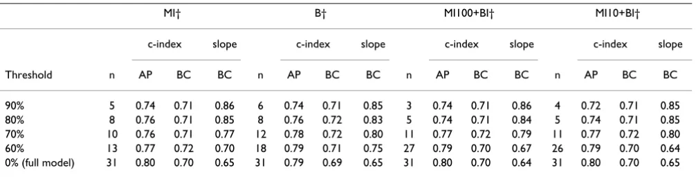
Table 3 summarizes the performance of the models devel-oped by the four methods where the p-value of 0.5 was used. It presents the number of variables included in the full model, and at inclusion levels of at least 90, 80, 70 and 60%. It also provides the corresponding discrimina-tive and calibradiscrimina-tive indices, respecdiscrimina-tively the c-index and the slope of the PI.
The reduced model, with prognostic indicators included whose inclusion frequency exceeds a threshold of 90% showed apparent c-indices between 0.72 and 0.74. The bootstrap corrected c-index was 0.71 for all four methods. These are relatively low values of the AUC, implying that these models do not distinguish patients with and with-out chronic low back pain very well. Including more
vari-Table 2: Inclusion frequencies and average rank per indicator selected by the four methods (MI = multiple imputations, B = bootstrap, M100+B = 100 imputations+bootstap, MI10+B = 10 imputations+bootstrap)
Method
MI† B† MI100+B† MI10+B† MI10 + B‡
% rank % rank % rank % rank % rank
Level of functional status at 3 months 100.0 1 100.0 1 99.4 1 99.5 1 88.0 3 Change in pain intensity 100.0 2 100.0 2 99.3 2 98.5 2 99.1 1 Pain at baseline 100.0 3 90.2 6 96.2 3 95.7 3 97.7 2 Physical activity 95.0 4 99.4 3 85.7 4 91.2 4 61.3 5 Vibration tools 90.0 5 94.2 4 81.0 5 80.9 5 43.7 13 Whole body vibration 88.0 6 71.0 12 77.2 7 79.6 6 50.2 4
Sitting 86.0 7 75.6 10 76.5 9 75.7 9 50.2 9
Job demands 81.0 8 65.6 16 77.7 6 79.0 7 52.2 8 Passive pain coping 77.0 9 51.8 30 71.8 11 72.5 11 41.1 15 Duration of complaints 70.0 10 71.2 11 76.5 8 77.4 8 35.9 19 Body mass index 63.0 11 90.8 5 66.1 13 69.0 14 39.2 16 Treatment during enrollment 62.0 12 85.8 7 75.5 10 75.5 10 46.2 11 Pain radiation 61.0 13 85.8 8 68.2 12 69.4 12 31.6 21 Working with hands under knee level 59.0 14 76.8 9 65.9 15 68.1 15 31.2 22 Education level 57.0 15 66.0 15 65.7 14 65.1 16 32.1 20 Job control 53.0 16 64.2 17 65.4 16 69.1 13 36.9 18 Quality of life 51.0 17 51.8 31 62.5 21 60.8 23 24.9 26 Bending and twisting of the trunk 50.0 18 56.8 22 64.6 17 62.9 17 45.9 12
Age 48.0 19 68.4 13 62.2 22 57.5 29 23.0 29
Lifting 48.0 20 66.6 14 61.4 24 60.4 25 41.8 14 Fear avoidance beliefs 48.0 21 55.8 26 63.3 19 61.8 21 25.4 25 Change in functional status 44.0 22 52.0 29 63.4 18 59.9 26 55.9 6 Kinesiophobia 43.0 23 52.8 28 63.2 20 60.4 24 22.6 30 Gender 42.0 24 56.2 24 61.5 23 61.5 20 24.6 27 Social support 41.0 25 56.0 25 60.0 26 62.8 18 27.9 24 Self-predicted certainty at 6 months 35.0 26 61.6 18 60.9 25 62.5 19 28.1 23 Active pain coping 32.0 27 54.4 27 59.9 27 58.6 28 23.5 28 Functional status at baseline 31.0 28 58.0 21 59.1 28 57.0 30 46.8 10 Stooping 30.0 29 58.8 19 57.7 30 59.4 27 53.0 7 Job satisfaction 29.0 30 58.4 20 58.2 29 60.9 22 37.7 17 Work absence at baseline 27.0 31 56.8 23 57.1 31 55.1 31 19.2 31
Rank: the sequence of indicators in order of their appearance into the backward regression models.
%: the proportion of times that the indicator is retained in the backward regression models (inclusion frequency). † P-value used of 0.5.
ables into the model increases the apparent c-index to 0.79–0.80, but a substantial part of the apparent increase of predictability is due to model optimism. By applying the bootstrap the c-index is adjusted to 0.69 and 0.70.
The slope of the PI is 0.86 for the simplest models (thresh-old 90%), but drops to 0.64 for the more comprehensive models. This means that the performance in new samples is likely to be affected, and that the more elaborate models are unlikely to achieve the apparent c-index of 0.77–0.79 when applied in new samples.
Given these results, a parsimonious prognostic model that accounts for both the missing data and variable selection variation will 1) shrink the regression weight by a factor of 0.85–0.86 and 2) lowers the apparent c-index to an adjusted estimate of 0.71, i.e., the value expected when the prognostic model is applied to new data.
Discussion
The effects of multiple imputation and bootstrapping on the inclusion frequency of prognostic indicators was investigated using four methods. For our data set, it appeared that multiple imputation lead to a relatively large spread in inclusion frequency, which is a nice prop-erty that eases decisions about which variables to include. In general, predictive models resulting from the combined methods were more similar to those generated by the imputation method than to those according to the boot-strap method. Incorporating variation from both the missing data and the model selection process revealed as much optimism as using either source alone. Optimism in the apparent c-index was larger for the more comprehen-sive models, i.e. when more variables are included who have a weak effect on the outcome in the models. The amount of bootstrap correction of the apparent c-index was almost independent of which sources of variation
were included. This also accounted for the slope of the PI, or the amount of shrinkage needed.
It is useful to account for sampling variation by bootstrap-ping, and this method is slowly gaining acceptance within the research community. Our study suggests that the boot-strap method alone might not be enough if the data set contains missing values. Many clinical data sets contain substantial amounts of missing data, but the influence of missing data on the inclusion frequency of prognostic var-iables used to select a model is hardly recognized [37]. In contrast to the study by Clarke and Altman that had fewer missing data [9], we found a substantial effect of imputa-tion on the apparent c-index estimate, especially for the more complex models. We therefore advocate the com-bined use of MI and bootstrapping, which addresses both imputation and sampling variation.
Note that some variables had over 45% of missing data. We nevertheless found that using 10 imputed datasets resulted in a similar selection of prognostic indicators than the use of 100 imputed datasets. This is in line with the claim of Rubin that 5 to 10 imputed datasets are enough to achieve high efficiency [6].
The bootstrap draws samples with replacement from the same data set. As was presented in table 2, the inclusion frequencies of the bootstrapping methods were less varia-ble than those of the MI method. Thus, bootstrapping in addition to MI in our study only led to a small increase in variation of the inclusion frequency. In general, sampling variation resulting from bootstrapping varies with respect to the sample size and the number of bootstrap samples drawn. The latter number must be high enough to mini-mize simulation variance. By using 200 bootstrap samples simulation variance decreases as well as the bias caused by these source of variance [38].
Table 3: The performance of methods 1 to 4 at different levels of proportions of selected indicators
MI† B† MI100+BI† MI10+BI†
c-index slope c-index slope c-index slope c-index slope
Threshold n AP BC BC n AP BC BC n AP BC BC n AP BC BC
90% 5 0.74 0.71 0.86 6 0.74 0.71 0.85 3 0.74 0.71 0.86 4 0.72 0.71 0.85 80% 8 0.76 0.71 0.85 8 0.76 0.72 0.83 5 0.74 0.71 0.84 5 0.74 0.71 0.85 70% 10 0.76 0.71 0.77 12 0.78 0.72 0.80 11 0.77 0.72 0.79 11 0.77 0.72 0.80 60% 13 0.77 0.72 0.70 18 0.79 0.71 0.75 27 0.79 0.70 0.67 26 0.79 0.70 0.64 0% (full model) 31 0.80 0.70 0.65 31 0.79 0.69 0.65 31 0.80 0.70 0.64 31 0.80 0.70 0.65
n: number of indicators selected in the multivariable models. AP: apparent index
BC: bootstrap corrected index
To identify relevant prognostic variables in our study we applied automatic backward selection in combination with bootstrapping [14-17] methods which are frequently used for this purpose. It has been shown that automatic backward regression can lead to an unstable selection of prognostic indicators [10]. For this reason, Sauerbrei and Schumacher [14] proposed the use of bootstrapping methods in combination with automatic backward selec-tion. They ranked the chosen indicators on basis of their selection in the models. Except for the method where only imputation was used, we applied bootstrapping in combi-nation with automatic backward selection in all other methods as proposed by Sauerbrei and Schumacher [14]. However, we extended their method in two ways. First, we included an imputation step for dealing with the missing data. Second, we augmented their method to include esti-mates of a shrinkage factor.
In our study we found bootstrap corrected c-indexes around 0.71 for discrimination in the models developed by the combined methods. Austin and Tu [13] found a c -index of 0.82 for a model developed and validated by the use of only the bootstrap method containing variables which were chosen at level of 60%. However, unclear is if they presented the bootstrap corrected c-index. Other studies that used the bootstrap had c-indexes between 0.70 and 0.80 [10,39], and reported slope values within the range of 0.80 and 0.90, similar to our results. For our models that combined MI and the bootstrap, we found a large decrease in the slope at the threshold of 60% com-pared to 70%. At 70%, the slope values were 0.79 and 0.80, which decreased to 0.67 and 0.64 at the threshold of 60%. Simultaneously, the number of indicators in these models changed from 11 at the 70% level to 27 and 26 at the 60% level. Steyerberg (2001) [10] demonstrated that it is better to use a more complete model to derive a shrinkage factor to improve the generalization of results to future patients. On basis of this recommendation the c -index and the slope among the models in our study with the 70% threshold provides a reasonable trade-off. When a parsimonious model is more important a model that is chosen at a higher inclusion threshold, e.g. 90%, is a good alternative.
In our procedure, identification of strong predictors pre-cede in two steps: first a selection on basis of the p-value, then a selection based on the inclusion frequency. These steps are communicating channels. One strategy is to be fairly flexible in the first step using a p-value of 0.5 and apply a strict variable inclusion frequency level of 90% in step 2. Another strategy is to be strict in step 1 (e.g. take a p-value of 0.157 or 0.05) and take a more lenient value at step 2 (e.g. 70%). Preferably, both routes would produce the same final model, and if this is the case, this will lend credence to the model.
We assumed that the data were missing at random (MAR). It is, by definition, not possible to test the MAR assump-tion. The prognostic variables that we have included in our study are fairly comprehensive with respect to their importance in low back pain studies. Using all these data in the imputation model makes the MAR assumption plausible, even if the data are not missing at random [6]. It is therefore reasonable to assume that although some variables might be not MAR, this is ignored by the inclu-sion of other variables in the imputation model when MI is applied [8]. Furthermore, if there are deviations from the MAR assumption in the data set the question is to what extent this affects the final results. Collins et al. [40] showed in a simulation study that an incorrect MAR assumption only had a minor effect on estimates and standard errors in combination with MI. Van Buuren et al. [41] reported in several strongly MAR incompatible mod-els that the negative effects on estimates after MI were only minimal. On basis of these study results we are fairly con-fident that we have generated valid imputations and that we were able to make reliable inferences from our data. It has been shown in the literature that imputation of out-come variables using the predictors under study mini-mizes bias in the relationship between predictor and outcome [42,43]. In our data set also some values with respect to the outcome variable were missing. We there-fore choose to impute these missing values within the MI algorithm.
Specification of the full imputation model is preferable, but led to computational problems. We followed the guidelines as described by van Buuren et al. [31] and Clark and Altman [9]. These guidelines consist of a number of steps for predictor selection in the context of imputation. Note that such procedures are essentially ad-hoc, and thus open to further research.
A common rule of the thumb states that sample size should be at least 10 times the number of events. In our case, the events per variable (EPV) ratio was 4.4, which according to some would be too low for reliable modeling [44]. Observe however that our methodology takes sam-ple size fully into account and corrects for dangers of over-fitting that may result from small samples. Overover-fitting diagnostics in Table 3 present the effect of sample size on the final model, and may be used to correct the model. Our methodology thus appears to have advantages over other methods if the sample size falls below the EPV > 10 rule.
limi-tation to main effects models only. Royston and Sauerbrei have shown that it is straightforward to control for non-linear effects by using fractional polynomials within a bootstrapping context [45]. Our method can thus be adjusted to include relevant nonlinearities in the prognos-tic model. Allowing for interaction makes things more complicated, but there is nothing in our methodology that prevents the use of interactions. When desired, inter-action terms can be included by starting from the final main effect of the multivariable model. In principle, the imputation model should also contain the relevant inter-actions, but the specification of the imputation will become more cumbersome. Not much is known about the strength of the influence of omitting or including interactions on the final inference.
As far as we know, this is the first study that addresses both multiple imputation and sampling variation on the inclu-sion frequency of prognostic variables. The bootstrap method for investigating the model building is not new, but is still somewhat experimental. Chen and George (1985) [46] described this procedure more than 2 decades ago for the Cox model. Sauerbrei and Schumacher [14], and Augustin [47] extended this method by using the bootstrap to account for uncertainty in model selection as proposed by Buckland [48]. In our study we accounted for uncertainty in selecting a model by means of sampling variation. Sauerbrei and Schumacher [14], and Augustin et al. [47] tested their methods in data sets containing missing values using complete case analyses. Our study provides a more principled alternative.
Conclusion
Missing data frequently occurs in prognostic studies. Mul-tiple imputation, to handle missing data, and bootstrap-ping, to select prognostic models, are increasingly applied in prognostic modeling. Both are promising techniques, but both may also complicate the model building process. We showed that it is possible to combine multiple impu-tation and bootstrapping, thereby accounting for uncer-tainty in imputations and unceruncer-tainty in selecting of models.
Competing interests
The author(s) declare that they have no competing inter-ests.
Authors' contributions
MWH participated in the planning and design of the study, the statistical analysis and drafted the manuscript. SVB participated in the planning and design of the study and the statistical analyses. DLK participated in the plan-ning and design of the study. WVM participated in the planning of the study. HCWDV participated in the
plan-ning, design and supervision of the study. All authors read and approved the final manuscript.
Acknowledgements
We would like to thank two reviewers for their thoughtful comments on the manuscript and Han Anema, Ivan Steenstra, Bart Staal and Hynek Hlobil for providing their data. Martijn Heymans was supported by the Nether-lands Organisation for Health Research and Development. The funding body had no role in study design; in the collection, analysis, and interpreta-tion of data; in the writing of the manuscript; and in the decision to submit the manuscript for publication.
References
1. Staal JB, Hlobil H, Twisk JW, Smid T, Koke AJ, van Mechelen W:
Graded activity for low back pain in occupational health care: a randomized, controlled trial. Ann Intern Med 2004,
140:77-84.
2. Steenstra IA, Anema JR, Bongers PM, de Vet HC, van Mechelen W:
The effectiveness of graded activity for low back pain in occupational healthcare. Occup Environ Med 2006,
63(11):718-25.
3. Heymans MW, de Vet HC, Bongers PM, Koes BW, van Mechelen W:
The Effectiveness of High Intensity versus Low Intensity Back Schools in an Occupational Setting: a pragmatic ran-domised controlled trial. Spine 2006, 31:1075-82.
4. Schafer JL: Analysis of Incomplete Multivariate Data. London: Chapman & Hall; 1997.
5. Little RJA, Rubin DB: Statistical Analysis with Missing Data.
New York: John Wiley & Sons; 2002.
6. Rubin DB: Multiple imputation for nonresponse in surveys.
New York: John Wiley & Sons; 1987.
7. Wood AM, White IR, Hillsdon M, Carpenter J: Comparison of imputation and modelling methods in the analysis of a phys-ical activity trial with missing outcomes. International Journal of Epidemiology 2005, 34:89-99.
8. Brand JPL: Development, implementation and evaluation of multiple imputation strategies for the statistical analysis of incomplete data sets. Enschede: Print Partners Ipskamp; 1999. 9. Clark TG, Altman DG: Developing a prognostic model in the
presence of missing data – an ovarian cancer case study. Jour-nal of clinical epidemiology 2003, 56:28-37.
10. Steyerberg EW, Eijkemans MJ, Harrell FE Jr., Habbema JD: Prognos-tic modeling with logisPrognos-tic regression analysis: in search of a sensible strategy in small data sets. Med Decis Making 2001,
21:45-56.
11. Harrell FE Jr: Regression modeling strategies. Berlin: Springer; 2001.
12. Viallefont V, Raftery AE, Richardson S: Variable selection and Bayesian model averaging in case-control studies. Stat Med 2001, 20:3215-3230.
13. Austin PC, Tu JV: Bootstrap Methods for Developing Predic-tive Models. American Statistician 2004, 58:131-137.
14. Sauerbrei W, Schumacher M: A bootstrap resampling procedure for model building: application to the Cox regression model.
Stat Med 1992, 11:2093-109.
15. Hollander N, Augustin NH, Sauerbrei W: Investigation on the improvement of prediction by bootstrap model averaging.
Methods Inf Med 2006, 45:44-50.
16. Altman DG, Andersen PK: Bootstrap investigation of the stabil-ity of a Cox regression model. Stat Med 1989, 8:771-83. 17. Steyerberg EW, Eijkemans MJ, Harrell FE Jr, Habbema JD:
Prognos-tic modelling with logisPrognos-tic regression analysis: a comparison of selection and estimation methods in small data sets. Stat Med 2000, 19:1059-79.
18. van den Hoogen JMM, Koes BW, Deville W, van Eijk JthM, Bouter LM:
The prognosis of low back pain in general practice. Spine 1997, 22:1515-21.
19. van Poppel MN, Koes BW, van der Ploeg T, Smid T, Bouter LM: Lum-bar supports and education for the prevention of low back pain in industry: a randomised controlled trial. JAMA 1998,
279:1789-94.
Publish with BioMed Central and every scientist can read your work free of charge "BioMed Central will be the most significant development for disseminating the results of biomedical researc h in our lifetime."
Sir Paul Nurse, Cancer Research UK
Your research papers will be:
available free of charge to the entire biomedical community
peer reviewed and published immediately upon acceptance
cited in PubMed and archived on PubMed Central
yours — you keep the copyright
Submit your manuscript here:
http://www.biomedcentral.com/info/publishing_adv.asp
BioMedcentral
occupational health care. Scand J Work Environ Health 1999,
25:50-6.
21. Carlsson AM: Assessment of chronic pain. I. Aspects of the reliability and validity of the visual analogue scale. Pain 1983,
16:87-101.
22. Gommans IHB, Koes BW, van Tulder MW: Validity and responsiv-ity of the Dutch Roland Disabilresponsiv-ity Questionnaire. [In Dutch: Validiteit en responsiviteit van de Nederlandstalige Roland Disability Questionnaire]. Ned Tijdschr Fysioth 1997, 107:28-33. 23. Hildebrandt VH, Bongers PM, van Dijk FJ, Kemper HC, Dul J: Dutch
Musculoskeletal Questionnaire: description and basic quali-ties. Ergonomics 2001, 44:1038-55.
24. Baecke JA, Burema J, Frijters JE: A short questionnaire for the measurement of habitual physical activity in epidemiological studies. Am J Clin Nutr 1982, 36:936-42.
25. Karasek RA, Brisson C: The Job Content Questionnaire (JCQ): An Instrument for Internationally Comparative Assess-ments of Psychosocial Job Characteristics. Journal of Occupa-tional Health Psychology 1998, 3:322-355.
26. Bigos SJ, Battie MC, Spengler DM, Fisher LD, Fordyce WE, Hansson TH, Nachemson AL, Wortley MD: A prospective study of work perceptions and psychosocial factors affecting the report of back injury. Spine 1991, 16:1-6.
27. Swinkels-Meewisse EJ, Swinkels RA, Verbeek AL, Vlaeyen JW, Oost-endorp RA: Psychometric properties of the Tampa Scale for kinesiophobia and the fear-avoidance beliefs questionnaire in acute low back pain. Man Ther 2003, 8:29-36.
28. Waddell G, Newton M, Henderson I, Somerville D, Main CJ: A Fear-Avoidance Beliefs Questionnaire (FABQ) and the role of fear-avoidance beliefs in chronic low back pain and disability.
Pain 1993, 52:157-68.
29. Kraaimaat FW, Bakker A, Evers AWM: Pain Coping Strategies in chronic pain patients: the development of the Pain-Coping-Inventory list. Gedragstherapie 1997, 30:185-201.
30. Sauerbrei W: The use of resampling methods to simplify regression models in medical statistics. Applied Statistics 1999,
48:313-329.
31. Van Buuren S, Oudshoorn K: Flexible multivariate imputation by MICE. In Technical report Leiden, The Netherlands: TNO Quality of Life; 1999.
32. Van Buuren S, Boshuizen HC, Knook DL: Multiple imputation of missing blood pressure covariates in survival analysis. Stat Med 1999, 18(6):681-94.
33. Harrell F, Lee K, Mark D: Multivariate prognostic models: issues in developing models, evaluating assumptions and adequacy, and measuring and reducing errors. Stat Med 1996, 15:361-87. 34. Vergouwe Y, Steyerberg EW, Eijkemans MJ, Habbema JD: Validity of prognostic models: when is a model clinically useful? Semin Urol Oncol 2002, 20:96-107.
35. Van Buuren S: The Mice Library. 2000 [http://www.multiple-impu tation.com].
36. Harrell FE: Design: S-plus functions for biostatistical/epidemi-ological modeling, testing, estimation, validation, graphics, prediction and typesetting by storing enhanced model design attributes in the fit. 1997 [http://biostat.mc.vanderbilt.edu/ twiki/bin/view/Main/FrankHarrell].
37. Burton A, Altman DG: Missing covariate data within cancer prognostic studies: a review of current reporting and pro-posed guidelines. Br J Cancer 2004, 91:4-8.
38. Davison AC, Hinkley DV: Bootstrap Methods and Their Appli-cation. New York: Cambridge University Press; 1997.
39. Steyerberg EW, Eijkemans MJ, Van Houwelingen JC, Lee KL, Habbema JD: Prognostic models based on literature and indi-vidual patient data in logistic regression analysis. Stat Med 2000, 19:141-60.
40. Collins LM, Schafer JL, Kam CM: A comparison of inclusive and restrictive strategies in modern missing data procedures.
Psychol Methods 2001, 6(4):330-51.
41. Van Buuren S, Brand JPL, Groothuis-Oudshoorn CGM, Rubin DB:
Fully conditional specification in multivariate imputation.
Journal of Statistical Computation and Simulation 2006, 76:1049-64. 42. Crawford SL, Tennstedt SL, McKinlay JB: A comparison of anlaytic
methods for non-random missingness of outcome data. J Clin Epidemiol 1995, 48(2):209-19.
43. Rubin DB: Multiple imputation after 18+ years. Journal of the American Statistical Association 1996, 91:473-489.
44. Peduzzi P, Concato J, Kemper E, Holford TR, Feinstein AR: A simu-lation study of the number of events per variable in logistic regression analysis. Journal of Clinical Epidemiology 1996,
49:1373-1379.
45. Royston P, Sauerbrei W: Stability of multivariable fractional polynomial models with selection of variables and transfor-mations: a bootstrap investigation. Stat Med 2003,
22(4):639-59.
46. Chen CH, George SL: The bootstrap and identification of prog-nostic factors via Cox's proportional hazards regression model. Stat Med 1985, 4:39-46.
47. Augustin NH, Sauerbrei W, Schumacher M: The practical utility of incorporating model selection uncertainty into prognostic models for survival data. Statistical Modelling 2005, 5:95-118. 48. Buckland ST, Burnham KP, Augustin NH: Model selection: An
integral part of inference. Biometrics 1995, 53:603-618.
Pre-publication history
The pre-publication history for this paper can be accessed here: