R E S E A R C H A R T I C L E
Open Access
On the impact of nonresponse in logistic
regression: application to the 45 and Up
study
Joanna J. J. Wang
1,2,3*, Mark Bartlett
2,3and Louise Ryan
1,3,4Abstract
Background:In longitudinal studies, nonresponse to follow-up surveys poses a major threat to validity, interpretability and generalisation of results. The problem of nonresponse is further complicated by the possibility that nonresponse may depend on the outcome of interest. We identified sociodemographic, general health and wellbeing characteristics associated with nonresponse to the follow-up questionnaire and assessed the extent and effect of nonresponse on statistical inference in a large-scale population cohort study.
Methods:We obtained the data from the baseline and first wave of the follow-up survey of the 45 and Up Study. Of those who were invited to participate in the follow-up survey, 65.2% responded. Logistic regression model was used to identify baseline characteristics associated with follow-up response. A Bayesian selection model approach with sensitivity analysis was implemented to model nonignorable nonresponse.
Results:Characteristics associated with a higher likelihood of responding to the follow-up survey include female gender, age categories 55–74, high educational qualification, married/de facto, worked part or partially or fully retired and higher household income. Parameter estimates and conclusions are generally consistent across different assumptions on the missing data mechanism. However, we observed some sensitivity for variables that are strong predictors for both the outcome and nonresponse.
Conclusions:Results indicated in the context of the binary outcome under study, nonresponse did not result in substantial bias and did not alter the interpretation of results in general. Conclusions were still largely robust under nonignorable missing data mechanism. Use of a Bayesian selection model is recommended as a useful strategy for assessing potential sensitivity of results to missing data.
Keywords:45 and Up Study, Nonignorable missing, Nonresponse, Bayesian selection model, Sensitivity analysis
Background
Handling missing data and non-response represents one of the most methodologically challenging aspects of longitu-dinal survey research. The loss of cohort members over time can arise from failure to locate or contact them, or because members refuse to participate for various reasons. Missing data and nonresponse constitute problems for epidemiological studies for two main reasons. First, miss-ingness leads to the loss of observations and the reduction of sample size. This can result in a loss of statistical power
and an increase in variances of estimates. The second consequence of nonresponse is that estimates may become biased, because the decision to respond to a survey is rarely completely random. Those members who responded to the follow-up surveys may have different characteristics from the nonresponders. In fact, many studies have found non-response is commonly associated with demographics, socioeconomic status and health behaviours and conditions ([1–3]). Hence, the responders may not be representative of the original sample and estimated measures of associations between exposure and outcome based solely on responders can be biased ([4, 5]).
It is possible to adjust and accommodate for missing responses. To compensate for the loss of participants in * Correspondence:[email protected]
1School of Mathematical and Physical Sciences, University of Technology
Sydney, Ultimo, Australia 2The Sax Institute, Sydney, Australia
Full list of author information is available at the end of the article
longitudinal surveys, it is common to assign weights, usually derived from the probability of response, to the responders to ensure the distribution of the original population is properly represented by the responders [6]. A second commonly used approach is multiple imputation, where the missing values are imputed based on statistical models which produce estimated plausible values [7]. Studies that use these methods to account for nonresponse have not found serious bias in association estimates ([8–11]). However, results from analyses based on weighting and multiple imputation methods are generally valid under the assumption that the data are “missing at random”(MAR), which means that missing-ness depends only on the observed data. Apart from multiple imputation, another commonly used approach is full information maximum likelihood (FIML) method which estimates parameters directly using all the infor-mation contained in the incomplete data set by maximising the observed data likelihood. Another popular maximum-likelihood based missing data method is the expectation-maximisation (EM) algorithm, which estimates the parameters directly by iterating between the E step and the M step. Both FIML and EM assume MAR mechanism and multivariate normality for the joint distribution of all variables.
In many situations there may be a reason to believe that even after accounting for the observed information, responders still differ from non-responders. In other words, the process that generates missingness may be directly related to the values of the unobserved variables. For example, people with very low or very high incomes may choose not to reveal their salaries. In the longitu-dinal study that motivates this paper, it is reasonable to think that people who move to a new residence during the follow-up period may be less likely to respond to the follow-up survey. Such cases, assuming that the data are MAR, may yield biased results. A number of authors in recent years have discussed strategies to handle this so called informative missingness. For instance, Diggle et al. [12] proposed a selection model for continuous longi-tudinal data with informative drop-out, that combines a linear model for the outcome and a logistic regres-sion model for the drop-out process. Such selection models have also been explored by Scharfstein et al., Ibrahim et al. and Carpenter et al. [13–15], among many others. On the other hand, the pattern-mixture approach [16] models the distribution of data condi-tional on the missing data pattern. Applications of the pattern-mixture model include [17–19]. A com-prehensive review and discussion of these models can be found in [20–23]. Recently, Wang et al. [24] pro-posed a Bayesian sensitivity analysis to address the problem of missing response data in the context of logistic regression based on a longitudinal follow-up
study. They also showed how to quantify the likely impact of bias associated with informative missingness when naïve methods are used. In this paper, we illus-trate the use of this methodology in the context of the 45 and Up Study, using our results to make rec-ommendations for broader epidemiological practice.
The 45 and Up Study is a large-scale Australian cohort study of individuals aged 45 and over. Recruitment into the 45 and Up Study commenced in early 2006 and the first 45 and Up Study follow-up survey was administered in 2012. The cohort consists of more than 267,000 men and women aged 45 years and over from the general population of the state of New South Wales [25]. Extensive information was collected at baseline on demographic and social characteristics; personal health behaviours; general health related data such as known risk factors for major causes of morbidity and mortality and other likely confounding factors. The 45 and Up Study aims to provide researchers with reliable information on a wide range of exposures and outcomes of public health for informing policy to support healthy aging.
A rigorous evaluation of possible impact of nonresponse in the 45 and Up Study has not been attempted. This study aims to fill this research gap by identifying sociode-mographic, general health and wellbeing characteristics associated with nonresponse to the follow-up question-naire and assessing the extent and effect of nonresponse on statistical inference drawn from estimates based on the 45 and Up Study survey data. In particular, we allowed for the possibility that nonresponse was non-ignorable and we illustrate the use of Bayesian selection model approach [24] which allowed us to examine the sensitivity of our conclusions to different assumptions on the missing data mechanism. The results of this study provide insights into factors associated with nonresponse and methods that are useful for exploring and mitigating the consequences of nonresponse in the 45 and Up Study.
Methods
The 45 and Up study
The Sax Institute’s 45 and Up Study is a population-based sample from the state of New South Wales (NSW), Australia. Extensive demographic and social characteristics, personal health behaviour and general health-related data on individuals are collected. This provides researchers with reliable information on a wide range of exposures and outcomes of public health. The 45 and Up Study as a research resource will also give government the tools for evidence-based policy making to support healthy ageing.
oversampled individuals from rural areas and those aged 80 years and over. Participants consented to regular follow-up and linkage of their survey data to a range of health databases. Recruitment commenced in February 2006 and the full cohort of size 267,157 reached by December 2009. The response rate to the 45 and Up Study is about 18% and participants included about 11% of the NSW population aged 45 years and over. Detailed description of the 45 and Up Study can be found in [25].
The first follow-up of participants began in 2012 with 41,440 45 and Up Study participants invited to respond. Of these, 27,036 returned the follow-up questionnaire, resulting in a response rate of 65.2%. After excluding in-dividuals with missing values for baseline covariates, 32,037 individuals were included in this analysis with 21,750 of these being responders to the follow-up questionnaire.
Data collection and variables
The 45 and Up Study baseline and follow-up question-naires include demographic data such as age, postcode of residence, education, country of birth and type of housing, lifestyle factors including physical functional capacity, self-rated health condition and social support and marital status, employment status and household income. To explore the impact of nonresponse on mea-sures of association, we focus on an outcome related to dwelling-type change between baseline and the follow-up. The 45 and Up Study questionnaires ask respondents to describe their dwelling type as belonging to one of eight categories: house, flat/unit/apartment, house on farm, retirement village/self-care unit, nursing home, hostel for the aged, mobile home and other. Due to low counts in some categories of these variables, house and house on farm; retirement village, nursing home and hostel for the aged; mobile and other are combined. Similarly, outer regional, remote and very remote Accessibility/Remoteness Index of Australia (ARIA) categories are combined. Physical functional limitation was assessed using the RAND 36-Item Health Survey, Version 1.0, subscale. The subscale was scored as recommended in ‘Scoring Instructions for MOS 36-Item Short Form Survey Instrument (SF-36) [26]. Social connectedness was assessed using the Duke Social Support Index (DSSI) subscale and scored as recommended by [27]. As per Phongsavan et al. [28], due to the positively skewed distribution of the social connectedness scores, this variable was transformed into quartiles.
In this paper, the outcome of interest was change in dwelling type between surveys, which was assessed by comparing responses to the relevant questions between the baseline and the follow-up surveys. To gain a better understanding of the particular type of housing transi-tion, we focus on the case where the binary outcome represents transition into retirement village/nursing
home/hostel for the aged, limited to those 45 and Up participants who were not in these categories at baseline. For ease of exposition, we subsequently refer to the out-come of interest as “transition to residential aged care”, or sometimes simply “transition”. It is important to explore various demographics, socio-economic and health factors associated with this transition as the find-ings of this study provide useful insights into relocation behaviour as people age and implications for aging and housing policy and age care provision.
Statistical analyses
We will consider two statistical methods to adjust for non-response: inverse probability weighting using a propensity score and a Bayesian selection model. Both of these methods require a formulation of the model which predicts the probability of responding, given a set of observed covar-iates. As discussed below, the Bayesian selection model also allows for the possibility that missingness might depend on the unobserved response variable. We first conduct univari-ate chi-squared tests of association, to identify significant differences between responders and nonresponders in terms of demographic characteristics (age, gender, educa-tion qualificaeduca-tion, country of birth, area remoteness), well-being (self-rated health, level of mobility, social support), household income, carer status, marital status and dwelling type at baseline.
The propensity score, as defined in Little [29], is the conditional probability that an individual responds, given a set of covariates. Following convention, we use a multivariable logistic regression model with response to the follow-up as the outcome variable to estimate propen-sity scores. Those variables with significant univariate associations with response status were included in a multi-variable logistic regression. Variables with p-values > 0.05 were removed from the model in a stepwise fashion. The likelihood ratio test and model comparison using Akaike’s Information Criterion were used for variable selection. The final propensity score model comprises of the variables included in Table 1. These also formed the basis of the modelling for the nonresponse probability in the selection model described below.
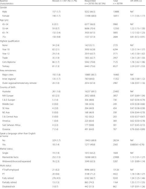
Table 1Characteristics of 45 and Up participants according to response to follow-up survey
Baseline characteristics
Movedn= 347 (%) (1.7%) Responded
n= 20730 (%) (67.3%)
Total
n= 30799
OR (95% CI)
Gender
Male 157 (1.7) 9232 (66.5) 13888 Ref
Female 190 (1.7) 11498 (68.0) 16911 1.11 (1.05–1.17)
Age (yrs)
45–54 6 (0.1) 6577 (66.0) 9960 Ref
55–64 59 (0.7) 8696 (70.4) 12350 1.22 (1.15–1.30)
65–74 132 (3.4) 3920 (67.5) 5805 1.12 (1.02–1.23)
75+ 150 (9.8) 1537 (57.3) 2684 0.81 (0.72–0.91)
Highest qualification
None 34 (2.4) 1421(52.1) 2725 Ref
Year 10 82 (2.1) 3950 (62.8) 6294 1.25 (1.14–1.37)
Year 12 29 (1.4) 2019 (63.7) 3171 1.45 (1.30–1.62)
Trade 35 (1.9) 1855 (62.7) 2957 1.34 (1.20–1.50)
Cert./diploma 86 (1.7) 5042 (70.8) 7125 1.78 (1.62–1.96)
Tertiary 81 (1.3) 6443 (75.6) 8527 2.29 (2.07–2.53)
Area remoteness
Major cities 192 (1.8) 10885 (66.1) 16460 Ref
Inner regional 135 (1.7) 7831(69.0) 11352 1.06 (1.00–1.12)
Outer regional/remote/very remote 20 (1.0) 2014 (67.4) 2987 1.06 (0.97–1.16)
Country of birth
Australia 261 (1.6) 16237 (69.1) 23492 Ref
NW Europe 65 (2.5) 2652 (68.8) 3857 0.97 (0.89–1.04)
S & E Europe 5 (1.4) 356 (48.8) 730 0.67 (0.56–0.79)
Middle East 0 (0.0) 106 (42.6) 249 0.50 (0.38–0.66)
SE Asia 4 (2.0) 204 (44.9) 454 0.47 (0.38–0.58)
NE Asia 0 (0.0) 168 (46.9) 358 0.56 (0.44–0.70)
S & Central Asia 0 (0.0) 102 (50.2) 203 0.50 (0.37–0.67)
America 1 (0.4) 223 (60.4) 369 0.62 (0.50–0.78)
Sub Saharan Africa 4 (2.3) 177 (58.8) 301 0.57 (0.45–0.72)
Oceania 7 (1.4) 491 (64.0) 767 0.76 (0.65–0.89)
Speak a language other than English at home
No 329 (1.7) 19453 (68.9) 28234 Ref
Yes 18 (1.4) 1277 (49.8) 2565 0.68(0.61–0.76)
Marital status
Single 19 (1.9) 1013 (63.2) 1604 Ref
Married/de facto 252 (1.5) 16368 (68.5) 23908 1.13 (1.01–1.27)
Widowed/divorced/separated 76 (2.3) 3349 (63.3) 5287 1.01 (0.89–1.14)
Work status
FT/self-employed 21 (0.2) 8996 (68.5) 13126 Ref
PT 20 (0.6) 3148 (71.2) 4422 1.18 (1.08–1.27)
Fully retired 276 (4.5) 6162 (66.7) 9243 1.34 (1.23–1.46)
Partially retired 13 (1.5) 865 (74.3) 1164 1.35 (1.17–1.55)
MAR assumption. That is, the probability of responding to the follow-up questionnaire is independent of the outcome, conditional on the set of observed covariates used to compute the weights. This is a strong assumption that asserts, given the observed covariates, those who do not respond behave in similar ways to those who do respond. This assumption is impossible to verify in practice without collecting data on the nonresponders.
For modelling the outcome variable, transition to resi-dential aged care facility, univariate Chi-squared analysis was firstly used to identify statistically significant associ-ations for each variable described above. Those variables with significant associations with the transition were included in a multivariable logistic regression model to further test associations. Possible first-order interaction
terms between the following variables were also consid-ered: sex with income, marital status, work status and age group; age group with physical function, health sta-tus, country of birth and language spoken at home. Interaction terms were first added to the main effects model one at a time and those with ap-value > 0.05 were dropped from the model. Then we sequentially add those interaction terms with significant p-values and after inclusion of main effects and other interaction terms, those withp-value > 0.05 were dropped to obtain the final model. This complete case analysis was re-peated with survey commands that allowed for weight-ing responders accordweight-ing to their propensity scored derived weights (“complete case with IPW”). Note that other variable selection methods due to shrinkage, such
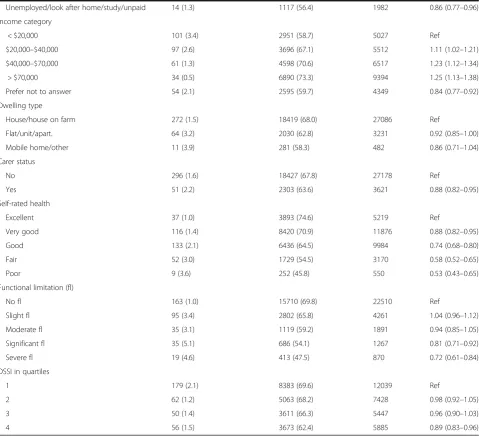
Table 1Characteristics of 45 and Up participants according to response to follow-up survey(Continued)
Unemployed/look after home/study/unpaid 14 (1.3) 1117 (56.4) 1982 0.86 (0.77–0.96)
Income category
< $20,000 101 (3.4) 2951 (58.7) 5027 Ref
$20,000–$40,000 97 (2.6) 3696 (67.1) 5512 1.11 (1.02–1.21)
$40,000–$70,000 61 (1.3) 4598 (70.6) 6517 1.23 (1.12–1.34)
> $70,000 34 (0.5) 6890 (73.3) 9394 1.25 (1.13–1.38)
Prefer not to answer 54 (2.1) 2595 (59.7) 4349 0.84 (0.77–0.92)
Dwelling type
House/house on farm 272 (1.5) 18419 (68.0) 27086 Ref
Flat/unit/apart. 64 (3.2) 2030 (62.8) 3231 0.92 (0.85–1.00)
Mobile home/other 11 (3.9) 281 (58.3) 482 0.86 (0.71–1.04)
Carer status
No 296 (1.6) 18427 (67.8) 27178 Ref
Yes 51 (2.2) 2303 (63.6) 3621 0.88 (0.82–0.95)
Self-rated health
Excellent 37 (1.0) 3893 (74.6) 5219 Ref
Very good 116 (1.4) 8420 (70.9) 11876 0.88 (0.82–0.95)
Good 133 (2.1) 6436 (64.5) 9984 0.74 (0.68–0.80)
Fair 52 (3.0) 1729 (54.5) 3170 0.58 (0.52–0.65)
Poor 9 (3.6) 252 (45.8) 550 0.53 (0.43–0.65)
Functional limitation (fl)
No fl 163 (1.0) 15710 (69.8) 22510 Ref
Slight fl 95 (3.4) 2802 (65.8) 4261 1.04 (0.96–1.12)
Moderate fl 35 (3.1) 1119 (59.2) 1891 0.94 (0.85–1.05)
Significant fl 35 (5.1) 686 (54.1) 1267 0.81 (0.71–0.92)
Severe fl 19 (4.6) 413 (47.5) 870 0.72 (0.61–0.84)
DSSI in quartiles
1 179 (2.1) 8383 (69.6) 12039 Ref
2 62 (1.2) 5063 (68.2) 7428 0.98 (0.92–1.05)
3 50 (1.4) 3611 (66.3) 5447 0.96 (0.90–1.03)
as the Least Absolute Shrinkage and Selection Operator (LASSO) can be applied. The complete case analysis and the complete case with IPW were performed using SAS version 9.3.
If the MAR assumption was violated, then IPW adjust-ment may not necessarily remove all nonresponse bias. This leads to the missingness mechanism known as “not missing at random” (NMAR) or informative missingness, where the probability of a missing value depends on the value of the variable that is missing. In this case, the missing data mechanism must be specified by the researcher and incorporated into the model in order to obtain unbiased parameter estimates. However, available data contains no information about what would be an appropriate model for the missing data and statistical inference is very sensitive to the choice of such model. This makes sensitivity analysis essential for investigating possible violations of the MAR assumption and exploring the robustness of the study con-clusions to increasingly extreme departures from the MAR mechanism ([24, 30–32]).
In this paper, we adopt a selection model approach for NMAR, which consists of two sub-models: one specifies the relationship between the covariates and the outcome of interest and the other represents the missing data process, which is dependent not only on observed covari-ates, but also the outcome. More specifically, we assume a standard logistic regression for the transition to residential aged care:
logitðP yð i¼1ÞÞ ¼b0þ
Xk
j¼1
bjxji; ð1Þ
whereyiis the outcome andxjiis thejth baseline covari-ate for subjecti. Potential covariates for the outcome, as well as those that may be predictors for nonresponse are detailed in Additional file 1. We then specify a logistic model for missingness as follows:
logitðP mð i¼1ÞÞ ¼θ0þX l
s¼1
θsxsiþλyi; ð2Þ
wheremiis a nonresponse indicator taking a value of 1 if the i th individual did not respond to the follow-up questionnaire, 0 otherwise. Other viable modelling frame-works for analysing data with informative missingness include pattern mixture models [33] and shared parameter models [34].
In the above selection model we assume a linear relationship between the logit of the probability of non-response and the outcome. Different values of the par-ameter λ posit different assumptions on how strongly the likelihood of nonresponse depends on the outcome. When λ= 0, we have the MAR case where the probabil-ity of nonresponse only depends on observed covariates.
This case corresponds exactly to the logistic regression model used to construct IPW weights and it further shows the selection model is an appealing choice as it relates to the propensity score method but model par-ameter are estimated jointly rather than in a two-stage process. More generally, the parameter λ is interpreted as the log odds ratio of nonresponse for those who had a dwelling-type change, conditional on all other covari-ates included in the model. We make the assumption that λ is nonnegative, that is, the likelihood of nonre-sponse is higher for those who had a dwelling-type change. This is a plausible assumption since change dwelling is often associated with family-type events such as marriage or birth and work transitions [35]. Thus, those who had dwelling-type change are more difficult to track in a longitudinal study as well as other sorts of changes in life course, making them less likely to re-spond to the follow-up survey [36]. In implementing the selection model, we repeat the analysis for a range of values of λ and examine the sensitivity of the estimated regression coefficients in the outcome equation across these values. The values we set for λ are (0, 1, 2, 3). More specifically, these values imply that the odds ratio of nonresponse for individuals with a dwelling-type change (which is transition into aged care facilities) is between 1 and 20 ([36, 37]). Note that in practice, one could also assign a mildly informative prior distribution toλand estimate it jointly with other model parameters. A full Bayesian probability modelling approach using Markov chain Monte Carlo (MCMC) was used for the selection model, as it was shown that the Bayesian mod-elling approach provides a flexible way to incorporate different assumptions on the missing data mechanism and enables coherent model estimation ([24, 38, 39]). We ran the selection model in the WinBUGS software [38, 40] for 15,000 iterations including 5000 for burn-in. Vague N(0, 1000) prior distributions were assigned to intercept parameters b0andθ0and all coefficientsbjand
θsin equations (1) and (2). Visual inspection of trace plots and autocorrelation plots of MCMC iterations was satis-factory suggesting that all runs achieved convergence.
Results
propensity score weights for responders and nonre-sponders are also presented in Table 1. Table 1 also pro-vides the percentages of subjects within each category who had transitioned to an aged facility at follow-up.
The results of the propensity score modelling show that individuals with the following characteristics have a higher probability of responding to the follow-up survey as compared with each reference category: female, in 55-74 age category, having higher educational qualifications, being married or in a de facto relationship and having higher household income. Conversely, those who at baseline survey worked full-time, had poor self-rated health, had significant to severe functional limitation, poor social connectedness, were a carer or were born outside Australia are more likely to be nonresponders at follow-up.
The mean propensity score for responders was 0.31 with a standard deviation of 0.11. The average weight given to each responder was 3.65 (range: 1.22 – 8.54). The C statistic or the area under the ROC curve for the model was equal to 0.65.
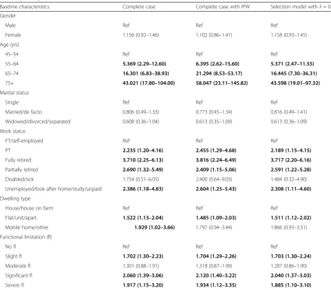
Table 2 shows ORs and 95% CIs for the complete case analysis (with and without IPW) and for the selection model with different values of λ for the association be-tween transition and various baseline characteristics. For the complete case analysis without any adjustment for nonresponse, the likelihood of making the transition is significantly greater for individuals who were over 55 years of age and who had slight, significant or severe physical functional limitation. On the other hand, those who worked full time or who lived in a house/house on farm were significantly less likely to transition into resi-dential aged care facility between baseline and follow-up. Table 2 reveals some interesting findings. First, results based on the propensity score analysis were very similar to those based on the naïve complete case analysis. Spe-cifically, there were only small changes in estimated ORs and no change in conclusions regarding associations with the transition of interest. The one exception was in the case with IPW, the likelihood of transition changed from borderline to non-significant for those living in mobile home/other as compared to those who lived in a house at baseline. In general, CIs were generally slightly wider for the propensity score-based analysis, due to the variability in the derived weights [41].
Second, Table 2 suggests that results based on the Bayesian selection modelling with λ= 0, were very close to the IPW and complete case analyses. This is to be expected since λ= 0 corresponds to MAR, as discussed above.
Finally, Table 2 provides a useful assessment of the po-tential impact of informative missingness by presenting results based on three different values of withλ. The de-gree of departure from MAR becomes more extreme as
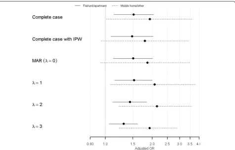
λ increases. For the most part, results were surprisingly robust, even for large values of λ. There were some cases, however, when the estimated ORs and conclusions changed. For example, the odds ratio for comparing the likelihood of transition into aged care facility between those who lived in mobile home/other to those lived in house at baseline became statistically significant under the NMAR assumption. The odds ratio estimates for baseline work status were significantly positive (except for “disable/sick”) in the complete case analysis, models assuming MAR and the selection model with λ= 1. However, asλincreases, the point estimates for categories “work part-time”, “partially retired” and “unemployed/ other”shifted toward the null value and became insignifi-cant when λ= 3. In contrast, the estimate for “disabled/ sick” shifted away from the null value and the CI no longer included 1 as λ increased. Lastly, for physical functional limitation, the only change in conclusion oc-curred for the category “moderate functional limitation”, where the estimate became significant in NMAR withλ≥2. Selected forest plots showing how OR estimates and CIs change under different modelling assumptions (i.e. complete case, MAR and NMAR with increasing values of λ) are shown in Figs. 1, 2 and 3. These plots clearly demonstrate the overall robustness of our conclusions to the possibility of MAR and NMAR assumptions, though we see some sensitivity of the estimates related to baseline work status. The remaining forest plots are available online as supple-mentary material (see Additional files 2, 3 and 4).
Combining the results of propensity score modelling in Table 1 and the OR estimates for the outcome variable under different assumptions as shown in Figs. 1, 2 and 3, it became clear that some variables are more sensitive to the underlying missing data mechanism and increasing departure from the MAR assumption. We are then able to classify these variables according to their sensitivity to the missingness assumptions and their strength of relationship with both the response and the outcome variable as shown in the following table.
Discussion
A major threat to the validity of longitudinal studies is nonresponse, which can potentially affect the magnitude and direction of measures of association and in turn can lead to erroneous conclusions. Using the baseline and follow-up data from the Sax Institute’s 45 and Up Study, we were able to identify a large number of factors associ-ated with response to the follow-up survey in this large cohort. More than 65% of the invited participants from the baseline responded to the follow-up survey.
qualification, married/de facto, worked part time or partially or fully retired and higher household income. Those who were born outside Australia, who spoke a language other than English at home, were a carer, who reported poorer subjective health, who had significant functional limitation and poor social connectedness were less likely to respond to the follow-up survey. There is no statistically significant difference in response by area remoteness and baseline dwelling type. Generally speak-ing, our findings on the characteristics associated with higher probability of response are in accordance with many previous studies [42, 43].
After assessing the factors associated with response to the follow-up survey, we then evaluated the extent to which nonresponse could impact the estimation of
change in dwelling type, in particular, transition into a residential aged care facility, between baseline and follow-up survey. To determine if estimates obtained from fitting a logistic model to complete cases only were affected by nonresponse, the first approach was to use propensity score to weigh each follow-up responder. The idea behind the weighting is that an individual with a low predicted propensity for response, who actually responded, will represent a larger group of individuals who did not respond. This approach has been used in many studies ([8, 44]) to assess nonresponse bias in cohort studies. Our results showed that adjusting for nonresponse by the means of using IPW had very little impact on the estimates of dwelling-type change related to various baseline characteristics.
Table 2Multivariate logistic regression analysis of characteristics associated with changed dwelling type between baseline and follow-up survey
Baseline characteristics Complete case Complete case with IPW Selection model withλ= 0
Gender
Male Ref Ref Ref
Female 1.156 (0.92–1.46) 1.102 (0.86–1.41) 1.158 (0.93–1.45)
Age (yrs)
45–54 Ref Ref Ref
55–64 5.369 (2.29–12.60) 6.395 (2.62–15.60) 5.371 (2.47–11.55)
65–74 16.301 (6.83–38.93) 21.294 (8.53–53.17) 16.445 (7.30–36.31)
75+ 43.021 (17.80–104.00) 58.047 (23.11–145.82) 43.598 (19.01–97.32)
Marital status
Single Ref Ref Ref
Married/de facto 0.806 (0.49–1.33) 0.773 (0.45–1.34) 0.816 (0.49–1.41)
Widowed/divorced/separated 0.608 (0.36–1.04) 0.613 (0.35–1.09) 0.613 (0.36–1.09)
Work status
FT/self-employed Ref Ref Ref
PT 2.235 (1.20–4.16) 2.455 (1.29–4.68) 2.189 (1.15–4.15)
Fully retired 3.710 (2.25–6.13) 3.816 (2.24–6.49) 3.717 (2.20–6.16)
Partially retired 2.690 (1.32–5.49) 2.409 (1.15–5.06) 2.591 (1.22–5.28)
Disabled/sick 1.754 (0.51–6.05) 2.400 (0.64–9.03) 1.484 (0.32–4.90)
Unemployed/look after home/study/unpaid 2.386 (1.18–4.83) 2.604 (1.25–5.43) 2.308 (1.11–4.60)
Dwelling type
House/house on farm Ref Ref Ref
Flat/unit/apart. 1.522 (1.13–2.04) 1.485 (1.09–2.03) 1.511 (1.12–2.02)
Mobile home/other 1.929 (1.02–3.66) 1.797 (0.94–3.44) 1.866 (0.93–3.51)
Functional limitation (fl)
No fl Ref Ref Ref
Slight fl 1.702 (1.30–2.23) 1.704 (1.29–2.26) 1.703 (1.30–2.24)
Moderate fl 1.301 (0.88–1.91) 1.318 (0.87–1.99) 1.287 (0.86–1.90)
Significant fl 2.060 (1.39–3.06) 2.120 (1.40–3.22) 2.040 (1.37–3.03)
Severe fl 1.917 (1.15–3.20) 1.934 (1.12–3.35) 1.885 (1.10–3.10)
The underlying assumption for using propensity score derived weights to adjust for nonresponse is MAR, which means the probability of nonresponse is independent of any unobserved data, conditional on the observed data. The MAR assumption is commonly used in the literature on missing data methods and an often used justification for MAR assumption is the availability of rich baseline information for characterising both responders and non-responders [45].
The use of a Bayesian selection model allows us to further assess the robustness of parameter estimates and conclusions when we have reasons to believe the missingness mechanism is NMAR or informative. In imple-menting the Bayesian selection model, we repeated our analysis over a range of fixed values of parameterλ, which controls the degree of departure from MAR assumption. [24] showed that it is not possible to estimate the parameter
λ and that the observed likelihood is nonidentifiable in the case of logistic regression with informatively missing out-comes. Hence we adopted a sensitivity analysis approach and repeated the analysis for various fixed values ofλ, which is equivalent to assigning a fixed point prior. The results from the selection model indicate that nonignorable nonresponse did not substantially affect estimates and conclusions regard-ing statistical significance of variables that were associated
with transition into residential aged care facility forλvalues which are not too extreme.
Table 3 shows that variables that are strong predictors for both the outcome and nonresponse are those af-fected to a greater extent by increasing departure from the MAR assumption. For instance, gender, marital status and baseline dwelling-type variables are quite robust to different missingness assumptions since they are weak predictors for either nonresponse or the out-come. Note that even with little change in magnitude, the estimate for those living in mobile home/other at baseline became significant in the NMAR analysis.
Due to low counts in this category, this result is of borderline insignificance under MAR assumption des-pite large estimated effect combined with wide CIs. A similar explanation is given for the category “moderate limitation” in the functional limitation variable, where small change in estimate caused the conclusion to change. On the other hand, age and work status as strong predictors for both nonresponse and the out-come, have their estimates varied substantially with in-creasing λ values. However, even with a large change in the estimates of the age variable, conclusions remain unchanged due to large magnitude of the estimated ORs and tight CIs.
This high level of robustness in estimates is consistent with the findings in Wang et al. [24]. Using a simpler model with one binary covariate, they derived exact expressions for the bias in estimates when using complete cases only. From that, it was shown that if the covariate is a weak predictor for the response missing-ness, then the bias of its regression coefficient in the outcome equation diminishes.
In practice, we suggest caution when interpreting re-sults for variables that are strong predictors for both nonresponse and outcome, as their estimates are sensi-tive to varying missingness assumptions and departure from the MAR assumption. On the other hand, small changes in estimates of variables which are not strong predictors of nonresponse and/or outcome could still result in change in conclusions when they are of border-line significance with wide CIs. Furthermore, change in conclusion usually occurs with large values of λ, which could be too extreme or scientifically implausible in a particular context.
Results based on our Bayesian selection modelling revealed a surprising level of robustness in terms of estimated ORs and associated CIs. A helpful explanation for this may be obtained through drawing an analogy with the familiar case control setting. There, it is well
known that oversampling cases does not affect estimated covariate effects, only the estimated intercept in a logis-tic regression analysis of a binary outcome. The presence of informative missingness in an epidemiological study means that responders and nonresponders are differen-tially represented in the study sample just as in a case-control study. Estimated ORs will only be affected if the missingness mechanism also depends on the same co-variates that we wish to correlate with the outcome of interest. This explains what we have observed in Table 2 and in the Figures, namely that estimated ORs are sensi-tive to informasensi-tive missingness only for covariates that are strong predictors of missingness as well.
Even though our results showed odds ratio estimates of the covariates and their CIs are generally robust to different assumptions on the missingness mechanism, the intercept estimate is affected, just like in a case-control setting as mentioned above. Hence, any compu-tation that requires the full set of parameter estimates such as calculating predicted probabilities would be im-pacted by the different assumptions.
Second, it is possible that there are some unmeasured factors associated with the outcome of interest and/or nonresponse which were not captured. However, since a large number of variables were collected at baseline, the likelihood of uncaptured confounders is low. Sensitivity analyses could be performed to assess how strong the effects of the unobserved confounder on the exposure and/or the outcome would have to be in order to over-turn a study conclusion [46]. Third, in our application we did not distinguish between different types of non-response. For example, reasons for nonresponse could include refusal or inability to be contacted. This can be accounted for by extending the model for nonresponse
by using multiple missingness indicators for each cause. Also, we restrict our analysis to individuals with fully observed covariates at baseline, those with missing values in any baseline covariate could be incorporated by using methods such as multiple imputation. Lastly, we conducted the sensitivity analysis for a range of λ values which we assume to be plausible for specifying the probability of nonresponse for individuals with and without transition into an aged care facility. Ideally we want to find strong scientific evidence to support the use of particular values ofλor to elicit expert knowledge about the odds of nonresponse for different dwelling change outcomes.
Conclusions
To the best of our knowledge, ours is the first study to investigate the impact of nonresponse in the 45 and Up Study cohort. We identified several baseline characteris-tics that were associated with high probability of nonre-sponse and many of them were commonly cited in the literature. By comparing odds ratio estimates for transi-tion into residential aged care facility using complete case analysis, inverse probability weighted method as-suming MAR and Bayesian selection model with the special case of MAR, our results showed in the context Fig. 3Odds ratio and 95% CI for dwelling type (Ref =“House”), under the complete case, complete case with IPW and selection model with different values ofλ
Table 3Classification of variables according to their strength of relationship with nonresponse and outcome
Predictor of nonresponse
Predictor of the outcome
Sensitivity to missingness mechanism
Variables
Strong Strong Yes Age; work status
Strong Weak No Gender; marital status
Weak Strong No Dwelling type;
physical functional limitation
-of examining factors associated with transition into aged care facilities, nonresponse did not result in substantial bias and certainly did not alter the interpretation of the results in general. We further examined the robustness of the conclusions under the NMAR assumption with varying degree of departure from MAR and showed the conclu-sions were still largely consistent for plausible values ofλ.
It is important to note that the MAR and NMAR clas-sification is unverifiable from the data under analysis and remains an assumption, hence making sensitivity analysis essential. Lastly, we describe in detail situations where the NMAR assumption and different values of λ are likely to affect parameter estimates and correspond-ing conclusions. We recommend caution when inter-preting results especially where variables are strong predictors for both nonresponse and the outcome, since their estimates and conclusions can be sensitive to the underlying missing data mechanism and varying degree of departure from the MAR assumption. Use of a Bayesian selection model is recommended as a useful strategy for assessing potential sensitivity of results to missing data.
Additional files
Additional file 1:Provides a table of description of selected variables collected in the 45 and Up Study baseline survey. (DOCX 28 kb)
Additional file 2:Provides a forest plot of OR estimates and CIs under different modelling assumptions for the variable“work status”. (EMF 135 kb)
Additional file 3:Provides a forest plot of OR estimates and CIs under different modelling assumptions for the variable“marital statuts”. (EMF 74 kb)
Additional file 4:Provides a forest plot of OR estimates and CIs under different modelling assumptions for the variable“functional limitation”. (EMF 120 kb)
Acknowledgements
This research was completed using data collected through the 45 and Up Study (www.saxinstitute.org.au). The 45 and Up Study is managed by the Sax Institute in collaboration with major partner Cancer Council NSW; and partners: the National Heart Foundation of Australia (NSW Division); NSW Ministry of Health; NSW Government Family & Community Services–Carers, Ageing and Disability Inclusion; and the Australian Red Cross Blood Service. We thank the many thousands of people participating in the 45 and Up Study.
Funding
This research received no specific grant from any funding agency in the public, commercial or not-for-profit sectors.
Availability of data and materials
The data that support the findings of this study are available from the Sax Institute and were used under license for the current study. Data are available for use by approved researchers.
Authors’contributions
JW conceptualised this project and drafted the manuscript and conducted the statistical data analysis. LR also conceptualised this project and provided overall guidance. MB and LR critically commented and revised the manuscript. All authors read and approved the final version of the manuscript.
Competing interests
The authors declare that they have no competing interests.
Consent for publication
The 45 and Up Study participants give consent on the understanding that reports and publications from the 45 and Up Study will be based on de-identified information and will not identify any individual taking part.
Ethics approval and consent to participate
The conduct of the 45 and Up Study was approved by the University of New South Wales Human Research Ethics Committee (HREC). The 45 and Up Study participants joined voluntarily and give consent for long term follow-up, including linkage to personal health records.
Publisher’s Note
Springer Nature remains neutral with regard to jurisdictional claims in published maps and institutional affiliations.
Author details
1School of Mathematical and Physical Sciences, University of Technology
Sydney, Ultimo, Australia.2The Sax Institute, Sydney, Australia.3The Australian Research Council Centre of Excellence for Mathematical and Statistical Frontiers (ACEMS), Parkville, Australia.4Department of Biostatistics, Harvard T.H. Chan School of Public Health, Boston, USA.
Received: 19 October 2016 Accepted: 27 April 2017
References
1. Nohr EA, Frydenberg M, Henriksen TB, Olsen J. Does low participation in cohort studies induce bias? Epidemiology. 2006;17(4):413–8.
2. Young AF, Powers JR, Bell SL. Attrition in longitudinal studies: who do you lose? Aust N Z J Public Health. 2006;30(4):353–61.
3. Hartge P. Raising response rates: getting to yes. Epidemiology. 1999;10(2):105–7.
4. Eagan TM, Eide GE, Gulsvik A, Bakke PS. Nonresponse in a community cohort study: predictors and consequences for exposure-disease associations. J Clin Epidemiol. 2002;55:775–81.
5. Shahar E, Folsom AR, Jackson R. The effect of nonresponse on prevalence estimates for a referent population: insights from a population-based cohort study. Ann Epidemiol. 1996;6:498–506.
6. Robins JM, Hernan MA, Brumback B. Marginal structural models and causal inference in epidemiology. Epidemiology. 2000;11:550–60. 7. Rubin DB. Multiple imputation for survey nonresponse. New York: John
Wiley & Sons Inc.; 1987.
8. Littman AJ, Boyko EJ, Jacobson IG, Horton J, Gackstetter GD, Smith B, Hooper T, Wells TS, Amoroso PJ, Smith TC. Assessing nonresponse bias at follow-up in a large prospective cohort of relatively young and mobile military service members. BMC Med Res Methodol. 2010;10:99.
9. Eerola M, Huurre T, Aro H. The problem of attrition in a Finnish longitudinal survey on depression. Eur J Epidemiol. 2005;20(1):113–20.
10. Boshuizen HC, Viet AL, Picavet HS, Botterweck A, van Loon AJ. Non-response in a survey of cardiovascular risk factors in the Dutch population: determinants and resulting biases. Public Health. 2006; 120(4):297–308.
11. Yu S, Brackbill RM, Stellman SD, Ghuman S, Farfel MR. Evaluation of non-response bias in a cohort study of world trade center terrorist attack survivors. BMC Res Notes. 2015;8:42.
12. Diggle P, Kenward MG. Informative drop-out in longitudinal data analysis (with discussion). J R Stat Soc Series C App Stat. 1994;43:49–93.
13. Scharfstein DO, Robins JM, Rotnitzky A. Adjustingfor nonignorable dropout using semiparametric nonresponse models (with discussion). J Am Stat Assoc. 1999;94:1096–146.
14. Ibrahim JG, Chen M-H, Lipsitz SR. Missing responses in generalized linear mixed models with then missing data mechanism is nonignorable. Biometrika. 2001;88:551–64.
16. Little R. Pattern-mixture models for multivariate incomplete data. J Am Stat Assoc. 1993;88:125–34.
17. Hedeker D, Gibbons RD. Application of random-effects pattern-mixture models for missing data in longitudinal studies. Psychol Methods. 1997;2:64–78.
18. Birmingham J, Fitzmaurice GM. A pattern-mixture model for longitudinal binary responses with nonignorable nonresponse. Biometrics. 2002;58:989–96. 19. Guo W, Ratcliff SJ, Have TT. A random pattern-mixture model for
longitudinal data with dropouts. J Am Stat Assoc. 2004;99:929–37.
20. Little R. Modeling the drop-out mechanism in repeated-measures studies. J Am Stat Assoc. 1995;90:1112–21.
21. Kenward M, Molenberghs G. Parametric models for incomplete continuous and categorical longitudinal data. Stat Methods Med Res. 1999;8:51–83. 22. Verbeke G, Lesaffre E, Spiessens B. The practical use of different strategies to
handle dropout in longitudinal studies. Drug Inf J. 2001;35:419–39. 23. Michiels B, Molenberghs G, Bijnens L, Vangeneugden T, Thijs H. Selection
models and pattern-mixture models to analyze longitudinal quality of life data subject to dropout. Stat Med. 2002;21:1023–42.
24. Wang JJJ, Bartlett M, Ryan L. On the impact of informative nonresponse in logistic regression. In: JSM Proceedings, health policy statistics section. Alexandria: American Statistical Association; 2016.
25. 45 and Up Study Collaborators. Int J Epidemiol. 2008;37:941–7. 26. RAND Health. Scoring Instructions for MOS 36-Item Short Form Survey
Instrument (SF-36). 2009. http://www.rand.org/health/surveys_tools/mos/ mos_core_36item.html. Accessed 3 May 2016.
27. Broadhead WE, Gehlbach SH, de Gruy FV, Kaplan BH. The duke-UNC functional social support questionnaire. Measurement of social support in family medicine patients. Med Care. 1988;26(7):709–23.
28. Phongsavan P, Grunseit AC, Bauman A, Broom D, Byles J, Clarke J, Redman S, Nutbeam D. SEEF Project. Age, gender, social contacts, and psychological distress: findings from the 45 and Up study. J Aging Health. 2013;25(6):921–43. 29. Little R. Survey nonresponse adjustments for estimates of means. Int Stat Rev.
1986;54(2):139–57.
30. Scharfstein DO, Daniels MJ, Robins JM. Incorporating prior beliefs about selection bias into the analysis of randomized trials with missing outcomes. Biostatistics. 2003;4:495–512.
31. Verbeke G, Molenberghs G, Thijes H, Lesaffre E, Kenward MG. Sensitivity analysis for non-random dropout: a local influence approach. Biometrics. 2001;57:7–14.
32. Kenward M. Selection models for repeated measurements with non-random dropout: an illustration of sensitivity. Stat Med. 1998;17:2723–32. 33. Little RJA. Pattern-mixture models for multivariate incomplete data.
J Am Stat Assoc. 1993;88:125–34.
34. Follmann D, Wu M. An approximate generalized linear model with random effects for informative missing data. Biometrics. 1995;51:151–68.
35. Lepkowski JM, Couper MP. Nonresponse in the second wave of longitudinal household surveys. In: Groves RM, Dillman DA, Entinge JL, Little RJA, editors. Survey nonresponse. NY: John Wiley and Sons; 2002. p. 121–34.
36. Voorpostel M, Lipps O. Attrition in the Swiss household panel: Is change associated with drop-out? J Off Stat. 2011;27:301–18.
37. Uhrig NSC. The nature and causes of attrition in the British Household Panel Survey. ISER Working Paper 2008-05. Colchester: Institute for Social and Economic Research, University of Essex.
38. Mason A, Best N, Plewis I, Richardson S. Insights into the use of Bayesian models for informative missing data. Technical report, Imperial College London. 2010.
39. Mason A, Richardson S, Plewis I, Best N. Strategy for modelling non-random missing data mechanisms in observational studies using Bayesian methods. J Off Stat. 2012;28:279–302.
40. Lunn DJ, Thomas A, Best N, Spiegelhalter D. WinBUGS–a Bayesian modelling framework: concepts, structure, and extensibility. Stat Comput. 2000;10:325–37. 41. Little R, Lewitzky S, Heeringa S, Lepkowski J, Kessler RC. Assessment of
weighting methodology for the National Comorbidity Survey. Am J Epidemiol. 1997;146:439–49.
42. Etter JF, Perneger TV. Analysis of non-response bias in a mailed health survey. J Clin Epidemiol. 1997;50:1123–8.
43. Watson N, Wooden M. Identifying factors affecting longitudinal survey response. In Methodology of longitudinal surveys, ed. Peter Lynn, 157-183. Chichester: John Wiley & Sons; 2009.
44. Seaman SR, White IR. Review of inverse probability weighting for dealing with missing data. Stat Methods Med Res. 2011;22:278–95.
45. Rao RS, Sigurdson AJ, Doody MM, Graubard BI. An application of a weighting method to adjust for nonresponse in standardized incidence ratio analysis of cohort studies. Ann Epidemiol. 2005;15:129–36.
46. Liu W, Kuramoto SJ, Stuart EA. An introduction to sensitivity analysis for unobserved confounding in non-experimental prevention research. Prev Sci. 2013;14:570–80.
• We accept pre-submission inquiries
• Our selector tool helps you to find the most relevant journal
• We provide round the clock customer support
• Convenient online submission
• Thorough peer review
• Inclusion in PubMed and all major indexing services
• Maximum visibility for your research
Submit your manuscript at www.biomedcentral.com/submit