A hybrid approach to the simultaneous eliminating of power-line interference and associated ringing artifacts in electrocardiograms

R E S E A R C H

Open Access

A hybrid approach to the simultaneous

eliminating of power-line interference and

associated ringing artifacts in electrocardiograms

Xiaolin Zhou

and Yuanting Zhang

* Correspondence:[email protected]

1

Institute of Biomedical and Health Engineering, Shenzhen Institutes of Advanced Technology, Chinese Academy of Sciences, Xili Nanshan, Shenzhen 518055, China Full list of author information is available at the end of the article

Abstract

Background:The second-order, infinite impulse response notch filter is widely used to remove electrical power line noise in electrocardiograms (ECGs). However this filtering process often introduces spurious ringing artifacts in the vicinity of raw signal with sharp transitions. It is challenging to simultaneously remove these two types of noise without losing vital information about cardiac activities.

Objective:Our objective is to devise a method to remove the power-line

interference without introducing artifacts nor losing vital information. To this end we have developed the "hybrid approach" involving two-sided filtration and multi-iterative approximation techniques. The two-sided filtration technique can suppress the interference but some cardiac components are lost. The lost information can be restored using multi-iterative approximation technique.

Results:For evaluation, four artificial data sets, each including 91 ECGs of different heart rates, were generated by a dynamical model. Four publicly-accessible sets of clinical data (MIT-BIH Arrhythmia, QT, PTB Diagnostic ECG, and T-Wave Alternans Challenge Databases) were also selected. Our new hybrid approach and the existing method were tested with these two types of signal under various pre-determined conditions. In contrast with the existing method, the hybrid approach can provide more than 27.40 dB and 37.77 dB reduction in signal distortion for 95% and 60% of artificial ECGs respectively; it can provide in excess of 11.78 dB and 17.48 dB reduction in distortion for 95% and 60% of these real records respectively.

Conclusions:Overall, a significant reduction in signal distortion is demonstrated. These test results indicate that the newly proposed approach outperforms the traditional method assessed on both the artificial and clinical ECGs and suggest it could be of practical use for clinicians in the future.

Background

Biopotential signals, such as electrocardiogram (ECG), often suffer from power-line interference (PLI, 50 or 60 Hz) since the recorded signal is an output of the electric fields of coupling states surrounding main power lines (PLs) and the power of the body. PLI is probably the most common problem encountered in the processing of biopotential signals. Essentially, a notch filter is adapted for minimizing PLI because of its ability to reject narrow band noise. Indeed, the second-order, infinite impulse re-sponse (IIR) notch filter is routinely applied for this purpose [1-3]. Because of the

transient response effect of the notch filter, the impulse response of this type filter gen-erally has an oscillatory behavior, which may cause microvolt-level ringing artifacts (RAs, typically ranging between 0 and 40 μV) in the immediate regions of input signal with sharp transitions. Besides, it will cause undesirable attenuation in signal compo-nents at frequencies close to the center frequency (50 or 60 Hz). Tolerable signal dis-tortion needs a narrow stopband bandwidth (SBW); however, a narrower SBW results in a longer transient response time (TRT); whilst a longer TRT often incurs more ser-ious RAs. It is an inherent contradiction. When an ECG signal is being processed, the RAs occur in the right side of QRS complexes, and consequently, this implies that many cardiac components are lost in ST-T regions. Serious distortion (signal distortion caused by the SBW itself and the appreciable RAs) may make the ECG signal more dif-ficult to interpret, particularly for the ST-T segment analysis, QT interval estimation, the detection of Ventricular Late Potentials (VLPs) and so on [4-6]. Removal of PLI however should be done with utmost stringent efforts not to eliminate or distort the raw signals without introducing artifacts nor losing vital information [7-9]. Many so-phisticated digital methods have been investigated to cope with either 50 or 60 Hz interference [10-12], and they satisfy the requirement for suppression and even elimin-ation of PLI during ECG signals acquisition. However, it is impossible to design an IIR notch filter to remove PLI without causing distortion [13-15], and this problem is still unsolved in practice. In this paper we address the challenges to simultaneously remove the PLI and RAs without losing critical cardiac components by developing a new method which we call the "hybrid approach".

Being motivated by early pioneering work on investigating the RAs phenomena caused by the suppression of PLI, in this paper, the hybrid approach comprising two-sided filtration and multi-iterative approximation techniques, is proposed to simultan-eously minimizing the PLI and associated RAs. In the first instance, the two-sided fil-tration technique is partitioned into four steps, which are applied to eliminate the PLI, localize the RAs and remove them afterward, whilst handling the boundary effects which are caused by the practical causal filter. To deal with the inherent contradictions, next the multi-iterative approximation technique is accomplished in three steps, which are adopted to sequentially reconstruct the lost cardiac information. A combination may thus prove to be more effective in eliminating these two types of noise. The elab-orate scheme of the hybrid approach is stated in Sect. 3.

notch filter with the center frequency of 50 and 60 Hz, respectively. The first two groups that without PLs, are designed for quantitatively investigating the signal dis-tortion. The other two groups, which mixed with the artificial PLs, are chosen for evaluating the distortion in an environment with interference, together with examin-ing the capacities of the newly presented and old methods for removexamin-ing PLI. The re-lationship of SBW and TRT of notch filters has not been well delineated, to provide more insight in the next section we also detail the key properties of finite impulse re-sponse (FIR) and IIR notch filters, so that their properties can be compared with each other. Additionally, related RAs are quantitatively examined, and the challenges are outlined.

Problem statement

A digital notch filter is a band-stop filter that passes all frequency components except those lying within a narrow range centered on a center frequencyf0. The magnitude re-sponse of an ideal notch filter may be given as below,

Hd ejω

_¼ 1; ω ≠ω0

0; ω¼ω0

ð1Þ

whereω= 2πf/fsis the normalized digital frequency,ω0= 2πf0/fsis the normalized cen-ter frequency at _f0.fsis the sampling rate, and fis the specified frequency. In practice, the notch filter has a SBW at f0, that is, Δω= 2πΔf/fs. Δω and Δf are normalized and digital SBWs, respectively.

FIR and IIR notch filters

LetHf(z) denote the transfer function of a second-order, FIR notch filter,

Hfð Þ ¼z 1−2γz−1þz−2 ð2Þ

where γ= cosω0. Hf(z) is simple and easy to implement. However, a disadvantage in using this kind filter is that the SBW of Hf(z) is relatively large, which could not meet the specifications [19]. In order to be applicable at narrow SBW situations, a Hf(z) based second-order, IIR notch filter is then commonly used [3,20],

Hið Þ ¼z β0⋅

Hfð Þz 1−2γβ₀z−1_{þð1−λÞβ}

0z−2

ð3:aÞ

whereβ0= 1/(1 +λ) andλ= tan(Δω/2). We regulate 0 <λ< 1 in this study. Eq. (3.a) can be rearranged as follows,

Hið Þ ¼z b0þb1z

−1_þb

2z−2

a0þa1z−1þa2z−2 ð

3:bÞ

where a0= 1,b0=b2=β0, a1=b1=−2γβ0, anda2= (1−λ)β0. First providedγ≠ −1, Hi (z) contains two poles (α1andα2) inside the unit circle |z| = 1 atzcomplex plane,

α1;2¼β0⋅ γ

ffiffiffiffiffiffiffiffiffiffiffiffiffiffiffiffiffiffiffiffi

γ2þλ2₋₁ q

ð4Þ

Letx[n] andy[n] be the input and output signals at discrete timen, respectively. This filter can be implemented by the following difference equation,

y n½ ¼−X

2

k¼1

aky n½ −k þ X2

k¼0

bkx n½ −k ð5:aÞ

where the subscript krefers to the kth-order index ofHi(z). By deduction, in essence, Eq. (5.a) can be identified as follows,

y n½ ¼X

∞

k¼0

h k½ x n½ −k ð5:bÞ

whereh[k] represents the impulse response ofHi(z) (see Appendix A),

h k½ ¼

b0; k¼0

−a1

ð Þh k½ −1 þb1; k¼1 −a1

ð Þh k½ −1 þð−a2Þh k½ −2 þb2; k¼2 ⋮

−a1

ð Þh k½ −1 þð−a2Þh k½ −2; k

≥

> > > > < > > > > :

ð6Þ

Hi(z) is a stable system, since |a2| < 1 and |a1| < 1 +a2. WhenHi(z) contains a pair of complex valued poles or a single negative pole, h[k] will cycle back and forth between negative and positive during the transient state [21], which indicates thath[k] is associ-ated with an oscillatory behavior.

Recalling Eq. (5.b), let us consider a finite case, this can be written as,

y n½ ¼X

K

k¼0

h k½ x n½ −k ð7Þ

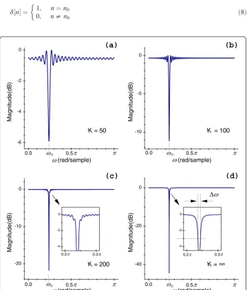
where K is a positive integer. One interpretation of Eq. (7) is that it represents a FIR notch system. Figure 1(a)-(d) display FIR and IIR notch filters calculated by Eqs. (6) and (3.b), respectively. Notably, the higher orderKof the filter, the weaker intensity the pass-band ripples and greater the selectivity. Consulting Figure 1(a)-(d), it is clear that this kind FIR filter has the following limitations: (A) The orderKis considerably higher than that of an equivalent second-order IIR filter meeting the same requirements. It thus has far more computational complexity. (B) Because of many pass-band ripples, signals that include the information of interest inside the relevant frequency bands will be grossly distorted. This is an issue related to the pseudo-Gibbs phenomena.

Inherent contradictions

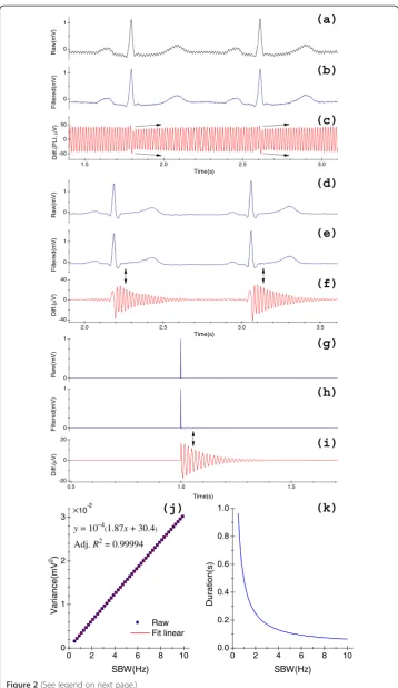
Just as in Figure 2(b), it seems as if there were no RAs. However, if we carefully check Figure 2(c) (as indicated by arrows), we find that they still exist.

Sharp transitions of signal may generate noticeable and intolerable RAs in the imme-diate vicinities of these abrupt changes. Figure 2(d)-(f ) is another example, in which we clearly see the spurious effect of RAs: RAs with the amplitude up to 30μV, as shown in Figure 2(f ). Therefore, the RAs should be carefully removed to prevent the distortion of input signal. The main cause of RAs is due to the abrupt bandstop ofHi(z), spectral components that lie within theΔf, as well as those close tof0±Δf/2, will be attenuated; this is the frequency-domain description. In the time domain, the cause of RAs isHi(z) itself: infinite impulse and oscillatory responses.

In order to quantitatively investigate the relationship between abrupt discontinuities of input signal and the corresponded RAs, we begin with the unit impulse signal, which is,

δ½ ¼n 1_0;; n¼n0

n≠ n0

ð8Þ

-6 -4 -2 0

-10 -5 0

-20 -10 0

-40 -20 0

-4 -2 0

-4 -2 0

0 0

0

0.0 0.0

0.0

0.5 0.5

0.5

K=

K= 200

K = 100

Magnitude(dB) Magnitude(dB)

Magnitude(dB) Magnitude(dB)

(rad/sample) (rad/sample)

(rad/sample) (rad/sample)

(a)

K= 50

0

(b)

0.0 0.5

0.3 0.2

0.3 0.2

(c)

(d)

∞

Δ

Figure 1Effects of different values ofK.(a) FIR filter withK= 50; (b) FIR filter withK= 100; (c) FIR filter

withK= 200; (d) IIR filter withK=∞; (a)-(c) are calculated by Eq. (6), respectively. (d) is calculated by Eq. (3.b), which is equivalent to Eq. (5.b). These notch filters are designed atfs= 500 Hz withf0= 60 Hz, and

0 1

0 1

0 1

0 1 0 1

0 1

2.0 2.5 3.0 3.5

-40 0 40

0 2 4 6 8 10

0 1 2 3

0 2 4 6 8 10

0.0 0.2 0.4 0.6 0.8 1.0

0.5 1.0 1.5

-20 0 20

1.5 2.0 2.5 3.0

-50 0 50

Raw(

mV)

(a)

Fi

lt

ered(mV)

(b)

Raw(

mV)

(g)

Fi

lt

ered(mV)

(h)

Raw(

mV)

(d)

F

ilte

re

d

(m

V

)

(e)

Time(s)

D

iff.(

V)

(f)

y= 10-4(1.87x+ 30.4)

Adj.R2= 0.99994

Raw Fit linear

SBW(Hz)

Variance(mV

2 )

(j)

×10-2

Du

ra

ti

o

n

(s)

SBW(Hz)

(k)

Di

ff

.(

V)

Time(s)

(i)

Time(s)

D

iff.(

P

L

I,

V)

(c)

where n0is a specific time. For simplifying the mathematics that follows the processing, by definition,δ[n] starts at 0 (n0= 0), and goes to∞. By makingδ[n] pass through the sys-temHi(z), and lettingyf[n] be the output,ν[n] =δ[n]−yf[n] the difference. The variance of ν[n] is then calculated by,

σ2 v¼

X∞

n¼0

v n½ 2¼X

∞

n¼0

δ½ n−X

∞

k¼0

h k½ δ½n−k

!2

¼ð1−h½ 0Þ2þX

∞

n¼1

h n½ 2

¼1−2h½ þ0 X

∞

n¼0

h n½ 2

ð9:aÞ

By deduction (see Appendix B), we relate theσ2 vandλ,

σ2 v¼

1 1−λ2⋅λ; σ

2 v∝Δf

ð9:bÞ

In most practical applications, provided γ2+λ2−1≤0 (i.e., tan(Δω/2)≤sinω0, com-monly,Δω/2≪ω0), then the pole radiusρforHi(z) is given by,

ρ¼j j ¼α1 j j ¼α2 pffiffiffiffiffia2¼

ffiffiffiffiffiffiffiffiffiffiffiffi

1−λ 1þλ

r

; Ifγ2_þλ2_{−1<0; Imα}

1¼−Imα2 ≠0

Ifγ¼−pffiffiffiffiffiffiffiffiffiffiffi1−λ2; α1 ¼α2<0

;ρ∝1=Δf

ð10Þ

Referring to Eqs. (9.b) and (10), we come to the overall conclusions: (i) If λ≪1, σ2 v can be loosely interpreted as a linear function of Δf. With Δf increasing, more and more signal components in the stop and pass bands will be modified in both the ampli-tude ("ripple") and the phase. (ii) Eq. (10) expresses that when Δf→0, thenρ→1. In other words, the wider the Δf, the closer the location of poles to the origin in the z

plane, meaning the system Hi(z) settles more rapidly (also meaning the system has a shorter duration of TRT) [22]. Therefore, it indicates that the duration of RAs tends to decrease asΔfincreases. It is an inherent contradiction of notch filters.

To visualize this problem, next we use Eq. (8) to generate a 10-second-length signal that is digitized at 1000 Hz, as shown in Figure 2(g). For convention, let the impulse occur atn0= 1 s (amplitude of the impulse is 1 mV). By makingΔfwith an increment of 0.1 Hz from 0.5 to 10.0 Hz, we calculated the outputsyf[n] by Eq. (5.a) atf0= 50 Hz

(See figure on previous page.)

Figure 2Results of processing of notch filtersHi(z).(a) Clinical ECG with 50 Hz real PLI; (b) The output

of this kind filter when applied to the signal in (a); (c) Differentiated components of (a) and (b); (d) Clinical ECG without PLI; (e) The output of the signal in (d) after passing it to this kind filter; (f) Differentiated components of (d) and (e); (g) A simulated unit impulse signal (1 mV); (h) The output ofHi(z) when applied to the signal in (g); (i) Differentiated results of (g) and (h); (j) The distributions ofσ2

vat various SBW; (k) The

with each Δf. We thus obtained 96 outputs. For each output, at a specifiedΔf, the dur-ation of RAs is defined as the time from impulse to the pointw, at which,

Xw

n¼0

δ½ n−yf½ n 2

= λ

1−λ2

≥95% ð11Þ

Figure 2(h) shows the output at Δf= 3.0 Hz, and Figure 2(i) displays the correspond-ing residual components. Figures 2(j) and (k) plot all the calculated results. Observe that these results agree with the aforementioned conclusions.

The principle of this algorithm

As we have seen, a cardinal implication is how the QRS complex affects the output of sys-temHi(z); to the system it always poses a big impulse. BecauseHi(z) is a causal filter, notice-ably time-decaying RAs can only occur on the right side of QRS complexes, see Figures 2 (e), (f), (h) and (i). This implies that RAs only depend on the input waveforms regardless of whether the output waveforms which are of steep transitions or not. In addition, Eqs. (9.b) and (10) offer insights on the determinants ofHi(z), which are uniquely controlled by itsΔf. These key intrinsic properties ofHi(z) would be applied in this newly developed approach.

As before, x[n] denotes the input, the number of samples is Land xT[n] denotes the counterpart of the signal _x[_n], that is, _xT[_n] =_x[_L−1−_n]. Then we construct a mirror extended signal,

xme½ ¼n x n½ ;

0 ≤n≤L−1

xT½n−L; L≤n≤2L−1

ð12Þ

We explore two-sided filtration and multi-iterative approximation techniques to eliminate the probable PLI and RAs which are contained inxme[n]. For the various fil-ter parmefil-ters, let yr

me½ n denote outputs of the signal xme[n] after passing it to the sys-temsHi(z),ymen ½ n denote outputs of this new method when applied toxme[n].

Two-sided filtration technique

The design procedure can be summarized as follows: Step 1 - Initialization

Givenfsandf0, at a specifiedΔf, we use Eq. (3.b) to calculate filter coefficientsa1,a2,b0,

b1andb2.bCons=⌊fs=fb⌋,⌊∙⌋represents a round operator,fb= 125 Hz is a constant.

bConsis an integer that is chosen to accommodate differentfs. IfbCons< 2, letbCons= 2. Step 2 - Twice notch filtering

(i) First notch filter suppressing. We pass thexme[n] to the notch filter, that is the Eq. (5.a) with filter coefficients calculated in the previous step, and get the output yr

me½ n as the system output. Then we can obtain the differential componentsdyme[n] using the derivative filter followed,

dy_me½ ¼n xme½ n−yrme½ n ð13Þ

-50 0 50

0.0 0.4 0.8

0.0 0.4 0.8

-10 0 10

-50 0 50

2.0 2.5 3.0 3.5

0 1

F

ilte

re

d

(m

V

)

(a)

Di

ff

.(

μ

V)

(b)

Di

ff

.(

μ

V)

(c)

Fi

lt

ered(

μ

V)

(d)

Fi

lt

er

ed(

μ

V)

(e)

Abs_Di

ff

.(

mV)

(f)

Abs_Di

ff

.(

mV)

(g)

C

o

e

ff.(

m

V

)

(h)

− −

+ +

D

iff.(

μ

V)

(i)

Fi

lt

er

ed(

m

V)

Time(s)

(j)

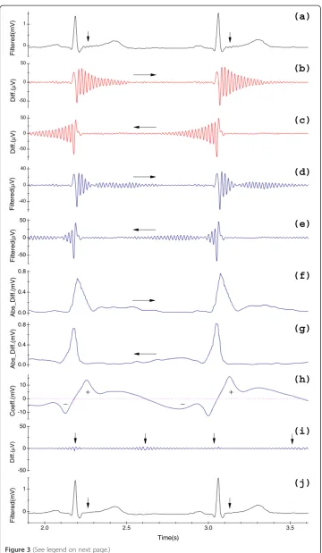
conducted in the counterpartxT[n], which is equivalent to be operated inx[n] in the backward direction, as displayed in Figure3(c), which shows the next half ofdyme[n] (L≤n≤2L–1) at relevant positions of the first half. The "relevant positions" means a sample atnis corresponded to the sample atn* (n* = 2L–1–n),

hereinafter the same. BecauseHi(z) is a causal system, detectable RAs in both halves ofdyme[n] lie on right and left arms of the same QRS complexes, respectively. (ii) Second notch filter suppressing. Sequentially, letdyme[n] be filtered by Eq. (5.a) with the same filter, we obtain the outputdy0_me½ n.dyme[n] may involove the PLI, RAs and distorted components which are caused by the boundary effect [3]. However,dy0me½ n can only contains the major information of RAs and distorted portions. Figure3(d) shows the first half ofdy0me½ n and Figure3(e) illuminates the second half ofdy0me½ n. In order to localize RAs in the next step, we need the second notch filtering operation. In fact, the possible PLI is directly suppressed in this step. Step 3 - RAs localization

Let us first construct a sequencecsme[n] implemented by the derivative operation as below,

csme½ ¼n dy 0 me½ n−dy

0

me½n−bCons

_ð14Þ

the time delay of Eq. (14) isbCons/2 samples. Next we letcsme[n] pass through a low-pass filter shown as follows, and letlsme[n] denote as the relevant output,

Hl0ð Þ ¼z

1−z−lOrder

1−z−1 ð15Þ

wherelOrder= 4∙bCons, intrinsic delay ofHl0(z) is (lOrder−1)/2 samples and the gain is

lOrder. For extracting the information of RAs, this low-pass filter is introduced to filter out fluctuations around the input sample and suppress undesirable outliers. Figure3(f) displays the first half oflsme[n] and Figure3(g) shows the second half. From Figures3(f) and (g), it is clear that triangle-like spikes localize the RAs.

Step 4 - Determination of the output

Likewise, we construct another sequencedsme[n], which results from the following operation,

dsme½ ¼n lsme½ n−lsme½ n ð16Þ

The use of Eq. (16) makes it possible to distinguish the RAs by means of positive and negative samples ofdsme[n]. Due to the same consideration inStep 3, we letdsme[n] be processed by another low-pass filter defined as below,

Hl1ð Þ ¼z 1−z

−jOrder

1−z−1 ð17Þ

(See figure on previous page.)

Figure 3Schematic diagram of the two-sided filtration technique.(a) The outputyr

me½ n of the notch

filterHi(z) when applied to the signal in Figure 2(d); (b) First half ofdyme[n]; (c) Another half ofdyme[n]; (d) First half ofdy0_me½ n; (e) Second half ofdy0_me½ n; (f)First half oflsme[n]; (g) Second half oflsme[n]; (h) Segment ofjsme[n]; (i) Residuesxme½ −n ymen ½ n; (j) The ultimate outputynme½ n of the signal in Figure 2(d) processed by

wherejOrder= 16∙bCons, the phase delay ofHl1(z) is (jOrder−1)/2 samples and gain is

jOrder, and letjsme[n] denote the output. Figure3(h) shows the first half ofjsme[n], and we see Figures3(b) and (c), it is obvious that to each sample at position n: (1) ifjsme[n] > 0, it represents that it gathers the information of RAs that lie within one arm of QRS complexes (left or right); (2) ifjsme[n] < 0, it means that it gather the information of RAs that lie within the other arm of QRS complexes (right or left), see Figures3(b), (c) and (h). Therefore, to each sample, we eliminate RAs based upon the criteria as below,

(i) Ifjsme[n] < 0,ynme½ ¼n yrme½ þn dy 0 me½ n; (ii) Ifjsme[n] > 0,ymen ½ ¼n yrme½ þn dy

0 me½ n;

(iii) Ifjsme[n] = 0 andlsme½n<lsme½n*,ynme½n=yrme½n+dy 0 me½n; (iv) Otherwise,yn

me½ ¼n yrme½ þn dy 0 me½ n:

Furthermore, another benefit of criteria (i)-(iv) is avoiding the boundary effect. Figure 3(j) shows the output yn

me½ n processed by this new method, and Figure 3(i) shows the residue portionxme½ n−ynme½ n. Pay special attention to the details of Figures 3 (a) and (j), and see the regions with arrows in Figure 3(j), then consult Figures 3(b), (c) and (i), we easily find that RAs are mostly eliminated. Note worthily, variablesbCons,

lOrder and jOrder are self-adaptive with respect to fs. Although the introduction of

both-sided filtration increases the memory requirements and the proposed method also increases the complexity by introducing logical tests in Step 4, two-sided filtration re-stores the phase distortions caused by the one-sided operation.

Multi-iterative approximation technique

The single implementation of previous technique has two minor drawbacks, both of which are presented in Figure 3(i): (1) it is based upon the assumption that RAs consist of non-overlapping portions at positions of both directions ofx[n]. In fact, it would not be able to distinguish overlapped RAs. However,Hi(z) of a smallΔfmay incur some ap-preciable parts (greater than 1 μV) overlapped in the middle of adjacent QRS com-plexes, as shown by the second and forth arrows in Figure 3(i). (2) Another major limitation encountered in using such a practical filter is that the system will attenuate waveforms constituted by high frequencies surrounding f0, as we see from positions with first and third arrows in Figure 3(i). As in the former disadvantage, intuitively, we might apply theHi(z) with a largerΔfto overcome this. From Eq (9.b), however, such a filter may cause more attenuation in signal components at frequencies close tof0, since the duration of RAs and the amount of lost components are mutually dependent upon each other.

A novel method that may overcome the fundamental problems is to repeat the pro-cessing of two-sided filtration several times with various Δf; we name it as multi-iterative approximation technique. Specifically, it can be partitioned into ternary steps as below,

drastically asΔfincreases at smallΔfcases; but it decreases slightly at largeΔfcases. Furthermore,σ2

v is roughly linear with respect to theΔf. Thus, an appropriate

compromise should be made to fit the task: an empirical and experimentalΔf= 6.0 Hz is employed here.

Inputxme[n] is depicted in Figure2(d). Figure4(b) illustrates the residual partxme½ n−ynme n

½ , which is obtained atΔf= 6.0 Hz, and Figure4(f) shows the related PSD spectrum. In the time domain, certain amounts of components of QRS complexes have been obviously lost, as we can see from Figure4(b). It can likewise be seen in Figure4(f) that parts of the signal of interest, which are close tof0, have been suppressed because of this largeΔfin the frequency domain.

Step II - Reconstruction of details with a small targetΔf. InStep I, we achieve a short duration of RAs, and thus RAs can be eliminated. However, because of the large SBW Δf, many cardiac components are lost. Thereby, in addition to possible PLs, residual partxme½ n−ynme½ n also contains lost components of original signal. In order to extract these useful details,xme½ n−ynme½ n is then to be processed by the two-sided filtration technique with a smallΔf(Δf< 6.0 Hz). Letxd

me½ ¼n xme½ n−ynme½ n denote the input, yd

me½ n the output.

Step IandStep IIare complementary with respect to Eqs (9.b) and (10). To illustrate,

Figure4(c) shows theydme½ n atΔf= 2.0 Hz and Figure4(g) displays the relevant PSD spectrum ofyd

me½ n. It can be observed from Figures4(b), (c), (f ) and (g) that most details have been reconstructed.

Step III - Reconstruction of slight details with the same targetΔf. We can see the vicinities indicated by arrows in Figure4(g),ydme½ n may still contain a little valuable information, just as the results shown in Figure4(c): the amplitude of which is greater than 1μV. To further reduce the distortion effects, similarly, letxs

me½ ¼n xdme½ n−ydme n

½ ,xs

me½ n is then be processed by the two-sided filtration technique with the sameΔf inStep II. Letysme½ n as the output. Figures4(d) and (h) showysme½ n and the relevant spectrum, respectively. We see that spectrum content in pass bands of Figure4(h) is flatter than that of Figure4(g), this represents that most lost details have been reconstructed, since the amplitude ofys

me½ n is substantially less than 1μV as shown in Figure4(d).

The ultimate output signal is derived from,

yn_me½ ¼n xme½ n− xsme½ n−ysme½ n

;ðn∈½0;L−1Þ ð18Þ

Figure4(a) displays the residual partxme½ n−yrme½ n obtained by the old method, and the relevant PSD spectrum is illustrated in Figure4(e). Observe that many cardiac components, which lie in the pass bands, have been removed, as illustrated at positions with the arrow in Figure4(e). By this new method, lost components have been minimized substantially in both time and frequency domains, as shown in Figure4(a)-(d) and Figure4(e)-(h), respectively.

Although one should aim to fully restore the lost components, it should be noted at this point that the residual coefficientsys

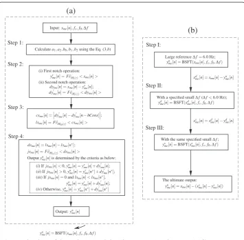
shows the flowcharts of the newly proposed algorithm; Figure 5(a) depicts the flowchart of two-sided filtration technique; Figure 5(b) represents the flowchart of multi-iterative approximation technique. Notably, Δfis the only parameter that needs to be specified in this method.

-30 0 30

-30 0 30

-2 0 2

2.0 2.5 3.0 3.5

-2 0 2

0 50 100 150 200 250 0

2k 4k

0 50 100 150 200 250 0

3 6

0 50 100 150 200 250 0

80 160

0 50 100 150 200 250 0

1 2

×10-6

×10-6

×10-6

D

iff.(

μ

V)

(a)

D

iff.(

μ

V)

(b)

D

iff.(

μ

V)

(c)

D

iff.(

μ

V)

Time(s)

(d)

PSD

int

ensi

ty

(

a.u.

)

Frequency(Hz)

(e)

PSD

int

ensi

ty

(

a.u.

)

Frequency(Hz)

(g)

PSD

int

ensi

ty

(

a.u.

)

Frequency(Hz)

(f)

×10-6

PSD

int

ensi

ty

(

a.u.

)

Frequency(Hz)

(h)

Figure 4Comparison of residual coefficients and relevant PSD spectra.(a) Thexme½ −n yrme½ n results

from the old method (Δf= 2.0 Hz); (b) Residual partxme½ −n ynme½ n inStep I(Δf= 6.0 Hz); (c) Residual part

yd

me½ n inStep II(Δf= 2.0 Hz); (d) Residual partysme½ n inStep III(Δf= 2.0 Hz); (e)-(h) show PSD spectra of

Materials and evaluation

Artificial and clinical ECG data sets

We simulated four artificial ECG data sets with fs of 250, 360, 500 and 1000 Hz, re-spectively. The generator generates realistic ECGs with user-settable parameters, such as "sampling frequency", "internal sampling frequency" and so on. This generator can be accessed from [16,17]. For this study, we used the generator to simulate 10-second-duration data at "internal sampling frequency" of 2000 Hz (but 720 Hz for ECGs sam-pled at 360 Hz) with the specified "mean heart rates", and regulated other parameters with default values [17]. To assess the performance of these two methods in an envir-onment with various sharp transitions, to each data set, we simulated ECGs with the "mean heart rates" ranging from 50 to 140 beats per minute (BPM), in increments of 1 BPM. We thus obtained 91 data for each data set.

Four widely used sets of real ECGs (MIT-BIH Arrhythmia Database [MITDB], QT Database [QTDB], PTB Diagnostic ECG Database [PTBDB], and the T-Wave Alternans Challenge Database [TWADB]) were also selected for evaluation [18], see Table 1 for details. All of these data were tested in this study.

(a)

(b)

Figure 5Flowcharts of the newly proposed algorithm.(a) Flowchart of the two-sided filtration

technique; (b) Flowchart of the multi-iterative approximation technique.Yout½n=Fi|HðzÞ<Xin[n]>

indicates that the inputXin[n] is filtered by the systemHðzÞ, and the relevant output isYout½n.

yn

Performance metrics

The main power supply is not perfectly stable. In some countries, tolerance of the fre-quency variation of PLs is 1% [23]. In poor electrical environments, however, the vari-ation may up to 3% [24]. Because the bandwidth of real PLs is varying, in order to assess the performance of this method under different situations, to both clinical and artificial data, we conducted these tests by changing Δfof the Hi(z) from 1.0 to 4.0 Hz with an increment of 0.1 Hz, respectively. In addition, to determine the capacity of eliminating PLI, artificial PLs that were simulated by sinusoidal functions (with the amplitude of 0.1 mV) at industrial frequencies (50 and 60 Hz, respectively), were added to the raw data. To each lead, at a specified Δf, different situations can be categorized into four groups:❶Atf0= 50 Hz, implementHi(z) without PLI;❷Atf0= 60 Hz, imple-ment Hi(z) without PLI;❸ At f0= 50 Hz, implementHi(z) with the addition of 50 Hz PLI;➍Atf0= 60 Hz, implementHi(z) with the addition of 60 Hz PLI.

We evaluated the relative distortion produced by two methods. The old method means the signals were only filtered by theHi(z). To each input signalx[n], we obtained the outputsyr[n] andyn[n] by processing input signalx[n] with the IIR filter, that is Eq. (5.a) and this new method, respectively. We calculated the relevant ratio of percentage root-mean-square difference (rPRD, in units of decibels [dB]), and it is given by,

rPRD¼10logPRD2r−10logPRD2n¼10log

σ2 r

σ2 n

ð19Þ

where PRD2r ¼ σ2

r

Am2, PRD2_n¼

σ2

n

Am2, Am2¼∑

L−1

n¼0x n½ 2

, σ2_r ¼L∑−1 n¼0 x n½ −y

r_{½ n}

ð Þ2

and σ2_n¼L∑−1 n¼0

x n½ −yn½ n

ð Þ2

.rPRDillustrates, for the new method, how distortion of the inputx[n] is quan-titatively lessened in comparison with the old method. It is not feasible to access the purely clinical signals, since these real signals might already contain PLs and other broadband noises. We hence let these signals be processed via the new approach first, and let the resulting signals be the inputsx[n] here.

To each data set with a specified group, wherein first, for the resultsrPRDs calculated from all of the various SBWs, we can figure out a threshold, at which, those results that, in excess of a certain percentage of total rPRDs, are greater than this threshold. Let rPRD|95% and rPRD|60%denote the thresholds with percentages of 95% and 60%, respectively. To facilitate comparisons with the old method in examining the capability

Table 1 Four publicly-accessible sets of clinical data are selected for evaluation

Databases fs(Hz) Data numbers/Channels (Durations)

Brief description

QTDB 250 105/2-lead It was chosen to represent a wide variety of QRS and ST-T morphologies.

(15 min.)

MITDB 360 48/2-lead It was obtained from 47 subjects and contains affluent arrhythmia information.

(30 min.)

TWADB 500 100/multi-lead Including subjects with risk factors, such as myocardial infarctins, transient ischemia, ventricular and so on, as well as healthy subjects.

(2 min.(appro.))

PTBDB 1000 549/15-lead It was collected from 290 healthy volunteers and patients.

of minimization of distortion at a specific SBW, then, for those resultsrPRDs outputted

by the same SBWΔf, at which (i.e., this singleΔf), we can define rPRDΔ50f% denote the

threshold with a percentage of 50%. Therefore,rPRD|95%,rPRD|60%and rPRDΔ50f%

rep-resent the overall performances of this newly prep-resented method.

Results and discussion

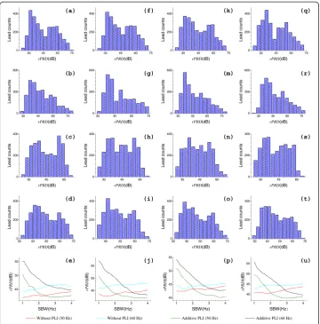
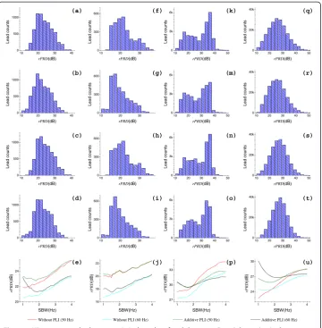
Test results of the artificial and clinical data sets are shown in Figures 6 and 7, respectively; where each histogram illustrates the results of a data set for a specific group. For each artifi-cial data set of a specific group, we have 2821 results calculated by Eq. (19). For a specific group, we have 6510, 2976, 28892 and 204228 results for QTDB, MITDB, TWADB and PTBDB, respectively. Insets, in the last rows of Figures 6 and 7, display the statistical results

(rPRDΔ50f%) corresponding to the histograms in the first four rows, respectively; for a

specific group with varying Δf, each curve is associated to a histogram in the same column. Tables 2 and 3 give the statistical results (rPRD|95%andrPRD|60%) corresponding to the histograms in Figures 6 and 7, respectively.

Figure 6(a)-(e) and Figure 7(a)-(e) plot the results using the artificial data set and QTDB (fs= 250 Hz), respectively. To groups❶ and ❷, asΔfincreases, it tends to

pro-duce largerrPRDΔ50f% for both artificial and clinical data sets as a whole. By contrast, to

both groups❸ and➍, asΔfincreases, it tends to producerPRDΔ50f% with relationships

that look like the exponential decay for artificial data sets, while relationships with

rPRDΔ50f% decreasing first and then increasing for QTDB data as a whole. With regard

to different notch frequencies, the performances are significantly different for both arti-ficial and clinical ECG data sets, as we see from Figures 6(e) and 7(e). From Table 2, to four groups, the minimum rPRD|95% and rPRD|60% were 28.82 dB and 38.82 dB for artificial ECGs, respectively. Similarly, in all of four groups, the minimum rPRD|95% and rPRD|60%were 15.07 dB and 20.58 dB for QTDB ECGs as shown in Table 3, re-spectively. It is worth noting that QTDB data was chosen specifically to contain a broad variety of QRS morphologies (i.e., various kinds of abrupt discontinuities) [25]. At this point, the results of QTDB ECGs are relatively more objective in the present study.

Figures 6(f )-(i) and 7(f )-(i) display the results using the artificial data set and MITDB

(fs= 360 Hz), respectively. Figures 6(j) and 7(j) are the relevant rPRDΔ50f% relations of

rPRD|95%andrPRD|60%were 28.91 dB and 38.75 dB for artificial ECGs, respectively; for the QTDB recordings with four groups, the minimum rPRD|95% and rPRD|60% were 11.78 dB and 17.48 dB, respectively.

The statistical results of artificial data set and TWADB (fs= 500 Hz) are shown in Figures 6(k)-(p) and 7(k)-(p), respectively. In terms of artificial ECG data with four groups, asΔfincreases, they exhibit consistent tendencies with these of artificial ECGs sampled at 250 and 360 Hz. However, for the TWADB data with four groups, as Δf in-creases, the performances depict no significant consistency as those of QTDB and

MITDB, since the rPRDΔ50f% are divergent at sides of low and large SBWs, while

rela-tively convergent in the middle of SBWs. In addition, for the QTDB and MITDB data sets, results with high probabilities lie in low sides of SBWs (i.e., less than 22 dB), but for the TWADB data the results of high probabilities lie within high sides (i.e., greater

30 45 60 75 0

200 400

30 45 60 75 0

300 600

30 45 60 0

200

400 400 400 400

30 40 50 60 70 0

200 400

1 2 3 4

45 50 55

30 45 60 75 0

200 400

30 45 60 75 0

300 600

30 45 60 0

200

40 50 60 70 0

200 400

1 2 3 4

45 50 55

30 45 60 75 0

200 400

30 45 60 75 0

300 600

30 45 60 0

200

30 40 50 60 70 0

200 400

1 2 3 4

40 45 50 55

30 45 60 75 0

200 400

30 45 60 75 0

300 600

30 45 60 0

200

30 40 50 60 70 0

200 400

1 2 3 4

40 45 50 55 Lead counts Lead counts Lead counts Lead counts Lead counts Lead counts Lead counts Lead counts Lead counts Lead counts Lead counts Lead counts Lead counts Lead counts Lead counts Lead counts rPRD(dB) (a) rPRD(dB) (b) rPRD(dB) (c) rPRD(dB) (d)

Without PLI (50 Hz) Without PLI (60 Hz) Additive PLI (50 Hz) Additive PLI (60 Hz)

rP R D (dB) SBW(Hz) (e) rPRD(dB) (f) rPRD(dB) (g) rPRD(dB) (h) rPRD(dB) (i) rP R D (dB) SBW(Hz) (j) rPRD(dB) (k) rPRD(dB) (m) rPRD(dB) (n) rPRD(dB) (o) rPRD (dB ) SBW(Hz) (p) rPRD(dB) (q) rPRD(dB) (r) rPRD(dB) (s) rPRD(dB) (t) rPRD (dB ) SBW(Hz) (u)

Figure 6Histograms and relevant statistical results of artificial data sets.From left to right: the four

than 30 dB). In Tables 2 and 3, for the four groups, we see that the minimum rPRD|95% and rPRD|60% were 27.88 dB and 38.60 dB, 14.66 dB and 24.86 dB, for artificial and TWADB data sets, respectively. Furthermore, from Figures 6(e), (j), (p) and Table 3, for this clinical data set, the performance of the new method is better than that of the QTDB and MITDB data sets as a whole.

10 20 30 40 0

500 1000

10 20 30 40 0

500 1000

10 20 30 40 0

500 1000

10 20 30 40 0

500 1000

1 2 3 4

20 22 24

10 20 30 0

300 600

10 20 30 0

300 600

10 20 30 0

300 600

10 20 30 0

300 600

1 2 3 4

16 18 20 22

10 20 30 40 50 0

3k 6k

10 20 30 40 50 0

3k 6k

10 20 30 40 50 0

3k 6k

10 20 30 40 50 0

3k 6k

1 2 3 4

27 30 33

10 20 30 40 50 0

20k 40k

10 20 30 40 50 0

20k 40k

10 20 30 40 50 0

20k 40k

10 20 30 40 50 0

20k 40k

1 2 3 4

24 27 30 Lead count s rPRD(dB) (a) Lead count s rPRD(dB) (b) Lead count s rPRD(dB) (c) Lead count s rPRD(dB) (d)

Without PLI (50 Hz) Without PLI (60 Hz) Additive PLI (50 Hz) Additive PLI (60 Hz)

rP R D (dB) SBW(Hz) (e) Lead count s rPRD(dB) (f) Lead count s rPRD(dB) (g) Lead count s rPRD(dB) (h) Lead count s rPRD(dB) (i) rP R D (dB) SBW(Hz) (j) Lead count s rPRD(dB) (k) Lead count s rPRD(dB) (m) Lead count s rPRD(dB) (n) Lead count s rPRD(dB) (o) rP R D (dB) SBW(Hz) (p) Lead count s rPRD(dB) (q) Lead count s rPRD(dB) (r) Lead count s rPRD(dB) (s) Lead count s rPRD(dB) (t) rP R D (dB) SBW(Hz) (u)

Figure 7Histograms and relevant statistical results of real data sets.From left to right: the four

columns, (a)-(e), (f)-(j), (k)-(p) and (q)-(u), show results of data sets withfsof 250, 360, 500 and 1000 Hz, respectively. For each data set, from top to bottom: the first four rows show results of four groups, including groups❶,❷,❸and➍, respectively. Four curves in each inset in the last row, which contains (e), (j), (p) and (u), correspond to four histograms in the same column and ordered by the legends, respectively.

Table 2 Statistical results of all of the four artificial ECG data sets

fs(Hz) Without PLI Additive PLI (0.1 mV)

f0= 50 Hz (−❶-) f0= 60 Hz (−❷-) f0= 50 Hz (−❸-) f0= 60 Hz (−➍-)

rPRD|95%

(dB) rPRD |60% (dB) rPRD |95% (dB) rPRD |60% (dB) rPRD |95% (dB) rPRD |60% (dB) rPRD |95% (dB) rPRD |60% (dB)

250 28.82 38.82 33.20 42.53 29.49 40.25 35.93 45.29

360 28.91 38.75 34.76 42.60 29.67 40.48 36.86 45.60

500 28.09 38.60 33.01 41.05 27.88 39.20 34.66 43.68

It can be clearly seen from Figures 6(q)-(u) and 7(q)-(u) that, for the artificial data set and PTBDB (fs= 1000 Hz), respectively, the results of the artificial ECGs reveal no sig-nificant difference compared with three earlier used artificial data sets. However, the

clinical ECGs have significant differences in the histograms as well as the rPRDΔ50f%

re-lations to these of three previous clinical ECGs. As far as the histograms of the four groups are concerned, they exhibit Gaussian probability distributions, since a huge number of results was obtained (a total of 204228 results) for each group, as shown in

Figure 7(q)-(t). In terms of rPRDΔ50f% relations, as shown in Figure 7(u), four curves

show tendencies toward convergence as Δf increases. Again from Tables 2 and 3, the minimum rPRD|95% andrPRD|60% were 27.40 dB and 37.77 dB for artificial ECGs of four groups, respectively; and for the PTBDB recordings, the minimumrPRD|95%and rPRD|60%were 14.67 dB and 23.85 dB, respectively.

Generally, for the artificial ECGs of a specific group, differences of results which were obtained from different data sets, show no special significance, since the only differ-ences of each data set are the sampling rates fsand the durationL. Regarding the four clinical ECG data sets (each including four groups), however, they showed obviously different performances, since these data sets were obtained from various subjects and with different emphases. In particular, the MITDB recordings, comprising many and a broad variety of wide size QRS complexes, show relatively poor performance. From all the results of artificial and clinical ECGs sampled at each fs, we can find that the per-formance exhibited by the artificial data set is significantly better than that of the rele-vant clinical data set. The reason is that the clinical ECGs may contain many low frequency leads. In summary, all of these test results indicate that the proposed method has the capacity to well reduce the PLI, and simultaneously, greatly minimize the RAs for both artificial and clinical ECGs.

Benefits and limitations

As previously mentioned, we always want the SBW of a notch filter to be very narrow for suppressing PLI. The FIR notch filter, which is defined by Eq. (7), does not encoun-ter the "infinite impulse" problem, but it requires a large degreeKto meet the specifica-tion, and this often comes at the cost of high computational complexity. Additionally, another problem with the FIR notch filter is that it may still produce RAs since it is os-cillatory in the range of the "finite response", because Kis a large number. In contrast,

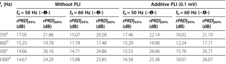
Table 3 Statistical results of all of the four clinical ECG data sets

fs(Hz) Without PLI Additive PLI (0.1 mV)

f0= 50 Hz (−❶-) f0= 60 Hz (−❷-) f0= 50 Hz (−❸-) f0= 60 Hz (−➍-)

rPRD|95%

(dB) rPRD |60%

(dB) rPRD |95%

(dB) rPRD |60%

(dB) rPRD |95%

(dB) rPRD |60%

(dB) rPRD |95%

(dB) rPRD |60%

(dB)

250a 17.05 21.86 15.07 20.58 17.46 22.14 16.02 21.10

360b 15.25 19.78 11.78 17.48 15.29 19.90 12.24 17.71

500c _{14.66 26.16 14.71 24.86 15.53 26.66 15.76 26.71}

1000d 14.67 24.20 15.88 23.85 16.58 25.38 18.07 26.07

a QTDB.b

MITDB.c TWADB.d

our hybrid approach provides primary benefits in eliminating specific interferences. It is not limited to reducing fixed fundamental PLI (50 or 60 Hz) but also applicable to removing the high-frequency harmonics for some worse cases, since the f0can be tai-lored to any desired frequency in this approach.

Thus far, all of our discussions are based upon the tan(Δω/2)≤sinω0. In certain ap-plications, however, some rare cases may still exist where tan(Δω/2) > sinω0, especially those ECG monitor systems with low sampling rates fs. In general, such situations occur atfs= 2f0+δfand 0≤δf≪fs. By Eq. (4), consider the following two possible cases,

(i)γ=−1 That is,f0=fs/2. According to Eq. (3.a),Hi(z) represents a first-order, IIR notch filter that has only one poleαinside the unit circle, for this case,

ρ0¼j j ¼α −α¼a2¼ 1−λ

1þλ; α<0;ρ 0

∝1=Δf

ð20Þ

Likewise, for the inputδ[n], we can obtain the output variance,

σ20 v ¼

1 1−λ2⋅λ; σ

20 v∝Δf

ð21Þ

Eqs. (20) and (21) demonstrate similar forms with Eqs. (10) and (9.b), respectively; it implies that the hybrid approach is also applicable. However, real PLs own a frequency bandwidth, the counterparts of PLs that lie within the right side off0will pollute valuable information of low frequencies. It is a limitation not caused by the method butfsitself. Therefore, we recommendδf≥4.0 Hz for practical application based upon the current study and literature [23,24].

(ii)−1 <γ< 0 andγ2+λ2−1 > 0 That is, |α1|≠|α2|. This yields (seeAppendix C),

Maxðj jα1;j jα2Þ ¼j jγ⋅

1þ

ffiffiffiffiffiffiffiffiffiffiffiffiffiffiffiffiffiffiffiffiffiffiffiffiffiffiffiffiffiffiffi 1−γ−2_þγ−2_λ2

q

1þλ ;

α1<0;α2<0;Maxðj jα1;j jα2Þ∝Δf

ð Þ

ð22Þ

Max(|α1|, |α2|) denotes the larger one of |α1| and |α2|. For |α1|≠|α2|, the settling time ofHi(z) is mainly determined by Max(|α1|, |α2|) [22]. Within this situation, using theHi(z) of a largerΔfwould not be able to achieve shorter durations of RAs but with more cardiac components lost. The "larger" referenceΔfis then set to the specified targetΔfinStep Ito meet the uniformity within the approach. Thus, it is worth emphasizing that more precautions should be taken whenΔfis adjusted to avoiding overlapping RAs in the middle of adjacent QRS complexes. Indeed, it is essential to remember this limitation as well, since Eq. (10) is not universal but with conditions.

Conclusions

the signal of sharp transitions by removing PLI is a great concern in the processing of biopotential signal. The detection and analysis of the VLPs in the ECG signal is highly sensitive to the residual PLI and the RAs after the QRS complexes as a result of the filtering technique applied. The artifacts may become considerable in cases of high and steep complexes. Owing to the intrinsic properties of Hi(z), we proposed a hybrid ap-proach, which utilizes Hi(z), to reliably suppress PLI as well as to aviod the generation of RAs. It is applicable to differentfsand easy to implement. In fact,Δfis the only par-ameter that needs to be specified for this approach. Problems are greatly mitigated via these techniques. Sufficient results and performance statistics are provided to validate the reliability of this method in the test environment with a variety of conditions (e.g., artificial and clinical ECGs, of various fs, with alteringΔf, etc.). An eventual consider-ation related to practice isf0of PLs. To the artificial PLs used in this study,f0was set to 50 or 60 Hz without varying. However, f0of real PLs, similar to its bandwidth, may fluctuate over a small range. Even so, we can refer to many previous studies for how to adaptive tracking of thef0with serious drift.

Appendix A: Proof of the Equation (6)

A real signal x[n] can be expressed as the sum of linear superposition of unit impulse functionsδ[n−k],

x n½ ¼X

∞

k¼0

x k½ δ½n−k ða:1Þ

where, if _k=_n, δ[_n−_k] = 1; otherwise, if _k≠_n, δ[_n−_k] = 0. By definition, to each im-pulse functionδ[n−k], the output is denoted as the impulse responseh[n−k]. Consult-ing Eq. (5.a), we obtain,

h n½ ¼−a1h n½ −1−a2h n½ −2

þb0δ½ þn b1δ½n−1 þb2δ½n−2 ð

a:2Þ

ProvideHi(z) is a causal system, then we conclude that,

(i)Ifn= 0,h[n−1] =h[n−2] = 0. Ignoreδ[n−1] andδ[n−2], sinceδ[n−1] =δ[n−2] = 0, then,

h n½ ¼b0 ða:3Þ

(ii)If_n= 1, because_h[_n−2] = 0, andδ[_n] =δ[_n−2] = 0, which results in,

h n½ ¼ð−a1Þh n½ −1 þb1 ða:4Þ

(iii)Ifn= 2,δ[n] =δ[n−1] = 0, we have,

h n½ ¼ð−a1Þh n½ −1 þð−a2Þh n½ −2 þb2 ða:5Þ

(iv)Ifn≥3, δ[n] =δ[n−1] =δ[n−2] = 0, this yields,

h n½ ¼ð−a1Þh n½ −1 þð−a2Þh n½ −2 ða:6Þ

Appendix B: Proof of the Equation (9.b)

The v[n] =δ[n]−yf[n] is equivalent to the inputδ[n] to be processed by the following comb filter,

Hcð Þ ¼z 1−Hið Þ ¼z c0⋅

1−z−2

a0þa1z−1þa2z−2 ð

b:1Þ

wherec0=λβ0. Ifγ≠ −1,Hc(z) also contains two poles atα1andα2inside the unit cir-cle |z| atzplane.

According to Parseval's theorem,σ2

vcan be calculated by,

σ2 v¼

X∞

n¼0

v n½ 2¼ 1

2π

Zπ

−π

Hc ejω

2

dω

¼ 1

2πj

∮

Hcð Þz Hcð Þz−1

z dz

ðb:2Þ

where∮crepresents the integral taken around the unit circle in counter-clockwise direc-tion, and let

F zð Þ ¼Hcð Þz Hc z −1 ð Þ

z ¼−

c20

z ⋅ ∏

2

i¼1

1−z2 z−αi

ð Þð1−αizÞ ð

b:3Þ

By the Residue theorem, we can obtain Eq. (b.4),

σ2 v¼

X2

k¼1

Res½F zð Þ;αk ðb:4Þ

By Eq. (b.3), we calculate residue valuesξandζat each pole,

ξ¼F zð Þ_z¼α1¼−c

2 0

α1⋅

1−α2 1

α1−α2

ð Þð1−α1α2Þ

ζ¼F zð Þ_z¼α2¼−c

2 0

α2⋅

1−α2 2

α2−α1

ð Þð1−α1α2Þ 8

> > > > < > > > > :

ðb:5Þ

And so,

σ2

v¼ξþζ¼c20⋅

1þa2

a2ð1−a2Þ¼

1

1−λ2⋅λ ðb:6Þ

Appendix C: Proof related to the Equation (22) For convention, we define,

ϕ¼1þφ

1þλ ðc:1Þ

where,

φ¼qffiffiffiffiffiffiffiffiffiffiffiffiffiffiffiffiffiffiffiffiffiffiffiffiffiffiffiffiffiffi1−γ−2_þγ−2_λ2 _ð

Take the derivative of both sides of Eq. (c.2) with respect toλ, which results in,

Δφ¼γ−2_φ−1_{λΔλ ðc:3Þ}

Then,

Δϕ¼ð1þλÞΔφ−ð1þφÞΔλ

1þλ

ð Þð1þλþΔλÞ

¼γ−2φ−1λð1þλÞ−ð1þφÞ

1þλ

ð Þð1þλþΔλÞ Δλ

¼ℱ_{Gð Þ}ð Þ_λλ Δλ

ðc:4Þ

where,

ℱð Þ ¼λ γ−2_{λð1þλÞ−φð1þφÞ} Gð Þ ¼λ φð1þλÞð1þλþΔλÞ

ðc:5Þ

First assume theℱ(λ)≤0 is true, from Eq. (c.5), this yields,

γ−2_{λð1þλÞ≤φð1þφÞ ðc:6Þ}

Solve Ineq. (c.6), we obtain (1 +λ)2≤0. Due to λ> 0, thus the assumptionℱ(λ)≤0 is false, thenℱ(λ) > 0. BecauseG(λ) > 0, we therefore have,

ℱð Þλ

Gð Þλ >0⇒Δϕ>0⇒ 1þ

ffiffiffiffiffiffiffiffiffiffiffiffiffiffiffiffiffiffiffiffiffiffiffiffiffiffiffiffiffi

1−γ−2þγ−2λ2 q

1þλ ∝Δf ðc:7Þ

Competing interests

The authors declare that they have no competing interests. Authors_’contributions

XZ developed the algorithm and drafted the manuscript. YZ provided suggestions and comments. All authors read and approved the final manuscript.

Acknowledgements

This work was supported in part by the National Basic Research Program 973 (2010CB732606), the Guangdong Innovation Research Team Fund for Low-Cost Healthcare Technologies in China, the External Cooperation Program of the Chinese Academy of Sciences (GJHZ1212), the Key Lab for Health Informatics of Chinese Academy of Sciences, the Enhancing Program of Key Laboratories of Shenzhen City (ZDSY20120617113021359) and the Young Scientists Fund of the National Science Foundation of China (61002002). The authors would like to thank Prof. Emma

Pickwell-MacPherson and Dr. Yan Chen for their assistance, advice, and encouragement. Author details

1

Institute of Biomedical and Health Engineering, Shenzhen Institutes of Advanced Technology, Chinese Academy of Sciences, Xili Nanshan, Shenzhen 518055, China.2_{Department of Electronic Engineering, The Chinese University of} Hong Kong, Shatin, NT, Hong Kong.

Received: 19 October 2012 Accepted: 1 April 2013 Published: 14 May 2013

References

1. McManus CD, Neubert KD, Cramer E:Characterization and elimination of AC noise in electrocardiograms: a comparison of digital filtering methods.Comput Biomed Res1993,26:48_–67.

2. Dotsinsky I, Stoyanov T:Power-line interference cancellation in ECG signals.Biomed Instrum Technol2005,

39(2):155_–162.

3. Pei SC, Tseng CC:Elimination of AC interference in electrocardiogram using IIR notch filter with transient suppression.IEEE Trans Biomed Eng1995,42(11):1128_–1132.

4. Breithardt G, Cain ME, El-Sherif N, Flowers NC, Hombach V, Janse M, Simson MB, Steinbeck G:Standards for analysis of ventricular late potentials using high-resolution or signal-averaged electrocardiography: a statement by a task force committee of the European Society of Cardiology, the American Heart Association, and the American College of Cardiology.J Am Coll Cardiol1991,17(5):999_–1006.

6. Subramanian AS, Gurusamy G, Selvakumar G:Detection of Ventricular Late Potentials using Wavelet-Neural Approach.Eur J Sci Res2011,58:11–20.

7. Kuchar DL, Thorburn CW, Sammel NL:Late potentials detected after myocardial infarction: natural history and prognostic significance.Circulation1986,74(6):1280–1289.

8. Prutchi D, Norris M:Design and development of medical electronic instrumentation.New Jersey: John Wiley E Sons, Inc; 2005.

9. Mousa A, Yilmaz A:Comparative analysis on wavelet-based detection of finite duration low-amplitude signals related to ventricular late potentials.Physiol Meas2004,25:1443–1457.

10. Van Alstk JA, Scbilder TS:Removal of base-line wander and power-he interference from the ECG by an efficient FIR filter with a reduced number of taps.IEEE Trans Biomed Eng1985,32(12):1052–1060. 11. Mitov IP:A method for reduction of power line interference in the ECG.Med Eng Phys2004,26:879–887. 12. Mahesh SC, Aggarwala RA, Uplane MD:Interference reduction in ECG using digital FIR filters based on

Rectangular window.WSEAS Trans Sig Proc2008,4(5):340–349.

13. Rangayyan RM:Biomedical signal analysis: a case-study approach.New York: IEEE press; 2002.

14. Kaur M, Singh B:Powerline Interference Reduction in ECG Using Combination of MA Method and IIR Notch.

IJRTE2009,2(6):125–129.

15. Luo S, Johnston P:A review of electrocardiogram filtering.J Electrocardiol2010,43(6):486–496. 16. McSharry PE, Clifford GD, Tarassenko L, Smith LA:A dynamical model for generating synthetic

electrocardiogram signals.IEEE Trans Biomed Eng2003,50(3):289–294.

17. ECGSYN:A realistic ECG waveform generator.http://physionet.cps.unizar.es/physiotools/ecgsyn/Matlab/. 18. The Physionet ECG Database: http://physionet.org/physiobank/database/.

19. Olguin DO, Lara FB, Chapa SOM:Adaptive notch filter for EEG signals based on the LMS algorithm with variable step-size parameter.InProceedings of the 39th International Conference on Information Sciences and Systems.Baltimore; 2005.

20. Hirano K, Nishimura S, Mitra S:Design of digital notch filters.IEEE Trans Commun1974,22(7):964–970. 21. Hellerstein J, Diao Y, Parekh S, Tilbury DM:Feedback control of computing systems.Chichester: Wiley-IEEE Press; 2004. 22. Vegte JVD:Fundamentals of Digital Signal Processing.New York: Prentice Hall; 2003.

23. Levkov C, Mihov G, Ivanov R, Daskalov I, Christov I, Dotsinsky I:Removal of power-line interference from the ECG: a review of the subtraction procedure.Biomed Eng Online2005,4:1–18.

24. Kumaravel N, Senthil A, Sridhar KS, Nithiyanandam N:Integrating the ECG power-line interference removal methods with rule-based system.Biomed Sci Instrum1995,31:115–135.

25. Laguna P, Mark RG, Goldberg A, Moody GB:A database for evaluation of algorithms for measurement of QT and other waveform intervals in the ECG.Comput Cardiol1997,24:673–676.

26. Press WH, Flannery BP, Teukolsky SA, Vetterling WT:Numerical recipes in C.Melbourne: Cambridge University Press; 1988.

doi:10.1186/1475-925X-12-42

Cite this article as:Zhou and Zhang:A hybrid approach to the simultaneous eliminating of power-line

interference and associated ringing artifacts in electrocardiograms.BioMedical Engineering OnLine201312:42.

Submit your next manuscript to BioMed Central and take full advantage of:

• Convenient online submission

• Thorough peer review

• No space constraints or color figure charges

• Immediate publication on acceptance

• Inclusion in PubMed, CAS, Scopus and Google Scholar

• Research which is freely available for redistribution