Shape‑based reconstruction of dynamic
fluorescent yield with a level set method
Xuanxuan Zhang
1, Jiulou Zhang
1, Jing Bai
1and Jianwen Luo
1,2*Background
Fluorescence molecular tomography (FMT) [1] is a promising imaging technique that
reveals the distributions of fluorescent agents within small animals in vivo. As an optical tomographic imaging technique, FMT has advantages of low cost, non-ionizing radia-tion and high sensitivity [2]. These merits lead to the popularity of the studies of FMT that not only observe static distribution of fluorescent markers [3] but also investigate metabolic process of drugs [4]. Compared with the static distribution, metabolic char-acteristics can provide additional information, which is important for drug development and tumor studies. At present, two kinds of methods are used in the reconstruction of dynamic FMT. The first one is to directly apply the reconstruction methods for static FMT to deal with dynamic cases [4, 5]. However, these methods are incapable of recov-ering the metabolic information within the data acquisition time and perform poorly especially when the fluorophore concentrations vary rapidly [6], because they only
Abstract
Background: Fluorescence molecular tomography (FMT) is an optical imaging tech-nique that reveals biological processes within small animals through non-invasively reconstructing the distributions of fluorescent agents. The primary problem in FMT with non-stationary fluorescent yield is the increase of the unknown parameters to be reconstructed. In this paper, a method is proposed to reconstruct dynamic fluorescent yield.
Methods: A shape-based reconstruction method that recovers dynamic fluorescent yield with a level set method is proposed for FMT. To reduce the number of unknown parameters, a level set function is introduced to describe the shape of target and a small number of parameters are used to describe the fluorescent yields at different time points.
Results: Results of simulations and phantom experiments demonstrate that the pro-posed method can recover well the dynamic fluorescent yields, shapes and locations of the target.
Conclusions: The proposed method can handle the cases with non-stationary fluores-cent yields and recover the fluoresfluores-cent yields at each projection angle.
Keywords: Fluorescence molecular tomography, Dynamic, Level set method, Shape-based reconstruction
Open Access
© 2016 Zhang et al. This article is distributed under the terms of the Creative Commons Attribution 4.0 International License (http:// creativecommons.org/licenses/by/4.0/), which permits unrestricted use, distribution, and reproduction in any medium, provided you give appropriate credit to the original author(s) and the source, provide a link to the Creative Commons license, and indicate if changes were made. The Creative Commons Public Domain Dedication waiver (http://creativecommons.org/publicdomain/ zero/1.0/) applies to the data made available in this article, unless otherwise stated.
RESEARCH
*Correspondence: [email protected]. edu.cn
2 Center for Biomedical
Imaging Research, School of Medicine, Tsinghua University, Beijing 100084, China
reconstruct a static distribution of fluorescent yield from data sets acquired within sev-eral minutes. The other kind of methods is based on different models. These methods model the metabolic process with a two-compartmental model [7, 8] or a polygonal line model [9, 10], and reconstruct the distributions of four pharmacokinetic parameters in the two-compartmental model or the distributions of fluorophore concentration vari-ation rate, instead of the distribution of fluorescent yield. These model-based methods convert the inverse problem of dynamic FMT from reconstructing a series of static dis-tributions of fluorescent yield to reconstructing the disdis-tributions of other parameters that can represent the metabolic information. Their limitations are the restriction of the used model. In this paper, a new approach is proposed to reconstruct dynamic fluores-cent yield based on a level set method. Different from the model-based methods, this method still reconstructs the distributions of fluorescent yield, thus the target metabolic curves are not restricted by specific models. This method is capable of recovering the distributions of fluorescent yield at each projection angle.
If the fluorescent yield is considered as the unknown parameter, the primary problem in FMT reconstruction with dynamic fluorescent yield is that the number of unknown parameters to be reconstructed is dramatically increased, because the fluorescent yield varies projection by projection in the dynamic problem whereas it does not change in the static problem. If the distributions of fluorescent yield at each projection angle are considered to be reconstructed, the number of unknown parameters will be multiplied by the number of projection angles (Np). Based on prior information that the same tissue or organ should have similar metabolic property, a shape-based reconstruction strategy is implemented in FMT to reduce the number of unknown parameters. In this strategy, the reconstructed object is divided into numbers of disjoint subregions and the shapes of these subregions are represented by a level set method [11] or spherical harmonics expansion [12]. Accordingly, the fluorescent yield in each subregion is described by only one parameter. It changes the reconstruction problem from reconstruction of fluores-cent yield at each voxel or node to reconstruction of level set function or expansion coefficients with several parameters of fluorescent yield. When a problem with dynamic fluorescent yield is considered, the number of unknown parameters will be reduced because the shapes of the distributions of fluorescent yield at different projection angles are described by the same set of unknown parameters by using the level set method or spherical harmonics expansion. In this paper, the level set method is chosen to represent the shapes of subregions for its ability of arbitrary boundary representation. Although spherical harmonics expansion can also describe arbitrary boundary theoretically, the maximum degree of spherical harmonics, which controls the shape representation, needs to be determined manually [13].
Methods
The generation and propagation of fluorescence in continuous wave FMT can be described by a couple of diffusion equations with Robin-type boundary condition, which are given by [14, 15]:
(1)
−∇D∇φx(r)+µaφx(r)=Q(r)
where Φ is the photon density. r denotes the coordinates and Ω denotes the region of imaged object. The subscripts x and m represent excitation and emission, respectively. Q is the excitation source term. n is the outward normal vector to the surface and q is a
term related to the optical reflective index mismatch at the boundary. μa and D are the absorption and diffusion coefficients, respectively. η is the quantum yield and μaf is the absorption coefficient of fluorophore to the excitation light. Their product is the fluores-cent yield which needs to be reconstructed.
Numerical approaches are commonly used to solve the diffusion equations with arbi-trary shaped domains. In this work, finite element method (FEM) is chosen to solve the forward problem, which converts the coupled diffusion equations given by Eq. (1) into the following linear equations after discretizing the imaged domain into a mesh with Nn nodes [16]:
Here Φ, X, and Q are column vectors with a length of Nn∙ X = ημaf is the vector of the unknown fluorescent yield. K is an Nn × Nn matrix which is commonly called stiffness matrix in FEM. F is a matrix with the same size as K, which is related to the excitation light field. K and F are constructed according to the topological structure of the mesh. K, F, and Q are given by:
where the subscripts i and j denote the indices of column and row, respectively. φi is the shape function at node i.
To reduce the number of unknown parameters, the shape-based reconstruction strat-egy is used. The imaged domain is assumed to consist of several disjoint subregions and the fluorescent yield in each subregion is represented by a single parameter. For simplic-ity, the case with two subregions (target region Rf and background region Rb) is con-sidered here and xf and xb are used to denote the corresponding fluorescent yields. To describe the shape of the subregions, a level set function is introduced [17]:
(2)
2qD∂φ (r)
∂n� +φ (r)=0 r∈∂�
(3)
Kφx = Q Kφm = FX
(4) Ki,j =
�
(D∇φi· ∇φj+µaφiφj)drn+ 1 2q
∂�
φiφjdrn−1
(5)
Fi,j =
�
φx(r)φiφjdrn
(6) Qi =
�
Q(r)φidrn
(7) x(r,t)=
where ψ is the level set function. Because the case with dynamic fluorescent yield is con-sidered, x, xf, and xb are functions of time.
In order to combine the level set function with FEM, ψ is discretized into an Nn dimensional vector Ψ of basis coefficients by a basis expansion with the shape functions as follows:
where ψi is the level set function at node i.
Then Eq. (7) is reformed by a single equation as follows:
where H (ψ) is the step function which is equal to 0 or 1 if ψ ≤ 0 or ψ > 0.
Through Eqs. (8) and (9), the unknown parameters to be reconstructed are converted from numbers of vectors X into only one vector Ψ with a set of values of fluorescent yields {xf (i)} and {xb (i)} after the discretization of the time t.
To reconstruct Ψ, {xf (i)} and {xb(i)} from boundary measurements, the following object function is defined:
where P is the measurement operation vector [18] used to extract the photon density at a certain detector point from the vector Φ. Nf denotes the number of frames of data used in the reconstruction and Nd denotes the number of detector points at each projec-tion angle. y* and y are the predicted measurements calculated from the forward
prob-lem and measurements acquired by the system, respectively. Differentiating Eq. (10) with respect to ψm yields:
where Ai (m) denotes the mth column of matrix K−1Fi∙ δ (ψm) is the Dirac function which is the derivation of the step function. xb (k, i) and xf (k, i) denote the fluorescent yield at the time point of the kth frame and ith projection angle for the background and fluores-cent target, respectively.
Accordingly, differentiating Eq. (10) with respect to xf (k, i) yields:
In Eq. (12), the indices of the nodes in Rf are needed, which are found with Ψ ≤ 0. The derivation with respect to xb (k, i) is similar to Eq. (12) whereas Rf is replaced by Rb.
(8)
ψ (r)=
Nn
i=1
ψiφi
(9) X(t)=xb(t)H(�)+xf(t)[1−H(�)]
(10)
Ŵ = 1
2 y ∗ −y 2 = 1 2 Nf
k=1
Np
i=1
Nd
j=1
PijK−1FiXk,i−yk,ij
2 (11) ∂Ŵ ∂ψm = Nf
k=1
Np
i=1
Nd
j=1
y∗k,ij−yk,ij
PijAi(m)xb(k,i)−xf(k,i)
δ(ψm)
(12) ∂Ŵ
∂xf(k,i) = Nd
j=1
y∗k,ij−yk,ij n∈Rf
The gradient of the object function consists of {∂Γ/∂ψm} and {∂Γ/∂xf|b (k, i)}. The gradient descent method [19] is used to reconstruct {xb (k, i)}, {xf (k, i)} and Ψ from measurements:
where the superscripts (n) and (n + 1) denote the indices of iteration. τ1 and τ2 are the
step lengths. They are determined empirically according to the value of the cost func-tion. Yk, i is the vector of measurements acquired at the kth frame and ith projection angle. J is the Jacobian matrix of the forward operator, which consists of row vectors {PijK−1Fi}. Because the Dirac function in Eq. (11) cannot be numerically calculated, it is omitted in the reconstruction. During the reconstruction, a low-pass filter [20] is applied to the reconstructed fluorescent yields after each iteration to smooth the curve of the reconstructed fluorescent yields.
Results and discussion
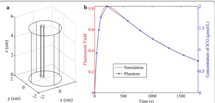
Simulation and phantom studies were implemented to validate the performance of the proposed method. The experimental setup of the simulation and phantom stud-ies is shown in Fig. 1. The imaged object was a cylinder with a diameter of 3 cm and height of 5.2 cm as shown in Fig. 1a. A tube with a diameter of 0.4 cm and height of 5.2 cm was inserted in the cylinder as the target. The tube was located at the position (x, y) = (0, 0.5) cm. In the simulations, a varied fluorescent yield according to the red
(13) �(n+1)=�(n)−τ1
Nf
�
k=1
JT
�
xb(k, 1)−xf(k, 1)
��
Y∗
k,1−Yk,1 �
.. . �
xb�
k,Np
� −xf�
k,Np
���
Y∗
k,Np−Yk,Np
�
(14)
x(fn|b+1)(k,i)=x
(n)
f|b(k,i)−τ2
k∈Rf|b
JiT(k)
Yk∗,i−Yk,i
curve shown in Fig. 1b was assigned to the tube. The curve was generated with a meta-bolic model of indocyanine green (ICG) [21]. Measurements were generated by Eq. (3) and 1 % Gaussian noise was added. In the phantom experiments, ten sets of measure-ments were acquired when different concentrations of ICG according to the blue points in Fig. 1b were filled in the tube. Then the dynamic measurements were synthesized by linear interpolation.
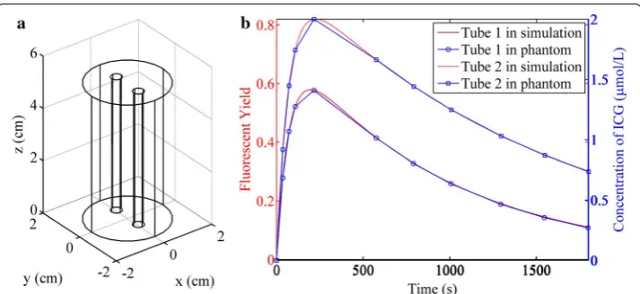
Simulations and phantom experiments on a model with double targets as shown in Fig. 2a were also implemented. Two tubes were inserted in the cylinder as the fluores-cent targets and the fluoresfluores-cent yields or confluores-centrations of ICG were set according to two different curves as shown in Fig. 2b. The heights and radii of the cylinder and tubes were the same as those in the previous experimental setting. The two tubes were away from each other with an edge-to-edge distance of 0.8 cm.
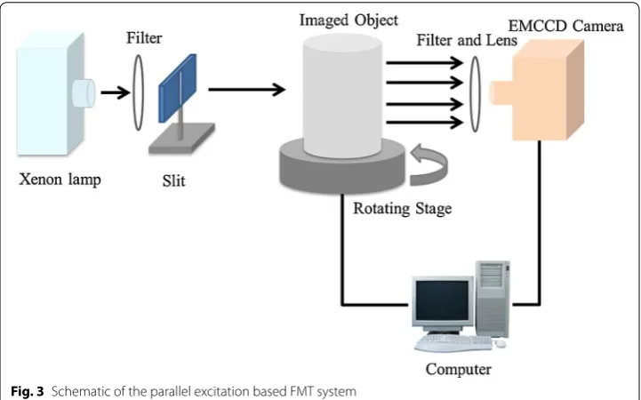
In the phantom experiments, 1 % intralipid with μs′ = 10.0 cm−1 and μa = 0.02 cm−1 was filled in the transparent cylinder. Accordingly, the same optical coefficients were used in the simulations. A parallel excitation based FMT system [22] as shown in Fig. 3 was used to acquire datasets in the experiments. The system consisted of three parts: excitation module, rotation stage, and detection module. The excitation module was
a 300 W xenon lamp (Asahi Spectra, Torrance, CA, USA) coupled with a 770 ± 6 nm
bandpass filter. A slit was used to generate a line illumination as the excitation source. The detection module consisted of a −70º cooled electron multiplying charge-coupled device (EMCCD) camera (iXon DU-897, Andor Technologies, Belfast, Northern Ire-land, U. K.), a Nikkor 60 mm, f/2.8D lens (Nikon, Melville, NY, USA), and an 840 ± 6 nm bandpass filter. The phantom was placed on the rotation stage between the excitation and detection modules and measurements were acquired at 18 projection angles over 360º illuminations and detections. The time for the data acquisition of each projection angle was 2 s. The same time interval was used in the simulations. After the detection of fluorescence, 72 white light images were acquired to recover the geometry of the imaged object with a surface reconstruction method [23].
In the reconstructions, the initial level set functions Ψ(0) were set as a small positive
constant for every node, but the value (i.e., 1) used in the phantom studies was chosen to be larger than the one (i.e., 0.001) used in the simulations because the data acquired by EMCCD and the data used in the simulations had different orders of magnitude. Since the level set functions were set to be homogenous at the beginning, the initial subregions consisted of only the background. The initial values of the fluorescent yield xb were set as 0 for all time points. It should be noticed that xf and xb cannot be the same, otherwise the gradient given by Eq. (13) would become 0. Therefore, the initial values of xf at each time point were set as 1000 and 0.1 for the phantom and simulation studies, respectively.
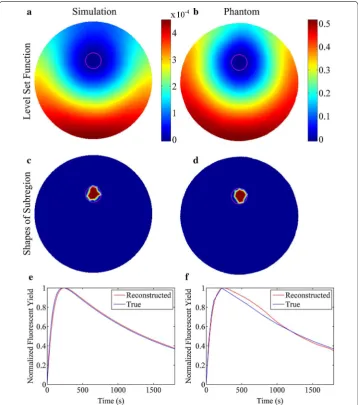
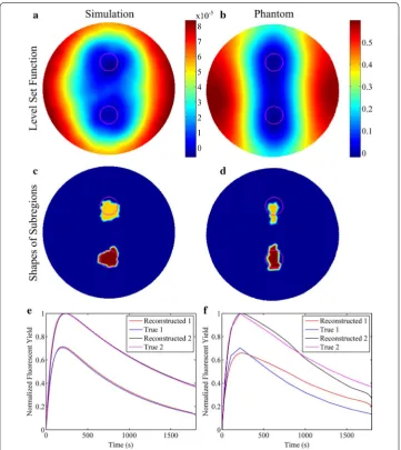
The reconstructions were restricted within a plane instead of the whole geometry for simplicity, due to the use of the line illumination, cylindrical phantom and tube. The reconstruction results at the center slice are shown in Figs. 4 and 5. The first and sec-ond columns of Figs. 4 and 5 are the results of the numerical simulations and phantom experiments, respectively. The subfigures (a) and (b) of Figs. 4 and 5 are the distributions of the level set functions reconstructed by the proposed method, while the subfigures (c) and (d) of Figs. 4 and 5 are the corresponding shapes of the subregions restricted by Ψ ≤ 0. The reconstructed fluorescent yields normalized by the maximum are shown in the subfigures (e) and (f) of Figs. 4 and 5 as time courses. The time interval between two neighbor fluorescent yields is equal to the time for the data acquisition of each projec-tion angle (2 s). It can be found that the reconstrucprojec-tions of both simulaprojec-tions and phan-tom experiments recover well the dynamic fluorescent yields, shapes and locations of the target. The reconstructed time course for the phantom experiments shows greater mismatch with the true one than that for the simulations, which is probably due to the complicated noise in the experimental datasets of different frames.
In this paper, the iteration formulas given by Eqs. (13) and (14) are derived from the gradient descent method. These formulas are similar to those derived from an artificial time evolution approach [11, 17, 24]. The Dirac function in the gradient for the level set
function is omitted in both the proposed method and the methods based on the artifi-cial time evolution approach. Rigorously, Eq. (13) is only proper for those locations with ψ = 0, because δ (ψ) is not zero only when ψ = 0. However, the gradient given by Eq. (13) shows the capability of finding the subregion of the target by decreasing the level set function with positive values until it becomes negative in numerical applications.
Conclusion
In general, a shape-based reconstruction method that recovers dynamic fluorescent yield with a level set method is proposed in this paper. This method is superior to the con-ventional method that reconstructs only a static distribution of fluorescent yield for the reconstruction of dynamic FMT, because it is capable of resolving the fluorescent yields
at each projection angle even if the fluorophore concentrations vary rapidly. Moreover, the target metabolic curves are not restricted by specific models.
Abbreviations
FMT: fluorescence molecular tomography; FEM: finite element method; ICG: indocyanine green; EMCCD: electron multi-plying charge-coupled device.
Authors’ contributions
XZ, JB, and JL designed the research. XZ developed the algorithm, analyzed the data and drafted the manuscript. XZ and JZ performed the simulation and phantom experiments. JZ and JL revised the manuscript. All authors have read and approved the final manuscript.
Author details
1 Department of Biomedical Engineering, School of Medicine, Tsinghua University, Beijing 100084, China. 2 Center for
Bio-medical Imaging Research, School of Medicine, Tsinghua University, Beijing 100084, China.
Acknowledgements
This work was supported by the National Basic Research Program of China (973) (2011CB707701), the National Natural Science Foundation of China (81227901, 81271617, 61322101 and 61361160418), and the National Major Scientific Instrument and Equipment Development Project (2011YQ03114).
Competing interests
The authors declare that they have no competing interests.
Received: 21 September 2015 Accepted: 6 January 2016
References
1. Ntziachristos V. Go deeper than microscopy: the optical imaging frontier in biology. Nat Meth. 2010;7:603–14. 2. Ntziachristos V. Fluorescence molecular imaging. Annu Rev Biomed Eng. 2006;8:1–33.
3. Shi J, Liu F, Zhang G, Luo J, Bai J. Enhanced spatial resolution in fluorescence molecular tomography using restarted L1-regularized nonlinear conjugate gradient algorithm. J Biomed Opt. 2014;19:046018.
4. Liu X, Liu F, Wang D, Bai J. In vivo whole-body imaging of optical agent dynamics using full angle fluorescence dif-fuse optical tomography. Chin Opt Lett. 2010;8:1156–9.
5. Liu X, Zhang B, Luo J, Bai J. 4-D reconstruction for dynamic fluorescence diffuse optical tomography. IEEE T Med Imaging. 2012;31:2120–32.
6. Liu X, Liu F, Bai J. A linear correction for principal component analysis of dynamic fluorescence diffuse optical tomography images. IEEE T Biomed Eng. 2011;58:1602–11.
7. Zhang G, Liu F, Pu H, He W, Luo J, Bai J. A direct method with structural priors for imaging pharmacokinetic param-eters in dynamic fluorescence molecular tomography. IEEE T Biomed Eng. 2014;61:986–90.
8. Zhang G, Pu H, He W, Liu F, Luo J, Bai J. Full-direct method for imaging pharmacokinetic parameters in dynamic fluorescence molecular tomography. Appl Phys Lett. 2015;106:081110.
9. Zhang X, Liu F, Zuo S, Shi J, Zhang G, Bai J, Luo J. Reconstruction of fluorophore concentration variation in dynamic fluorescence molecular tomography. IEEE T Biomed Eng. 2015;62:138–44.
10. Zhang X, Liu F, Zuo S, Zhang J, Bai J, Luo J. Fast reconstruction of fluorophore concentration variation based on the derivation of the diffusion equation. J Opt Soc Am A. 2015;32:1993–2001.
11. Schweiger M, Arridge SR, Dorn O, Zacharopoulos AD, Kolehmainen V. Reconstructing absorption and diffusion shape profiles in optical tomography by a level set technique. Opt Lett. 2006;31:471–3.
12. Wu L, Wan W, Wang X, Zhou Z, Li J, Zhang L, Zhao H, Gao F. Shape-parameterized diffuse optical tomography holds promise for sensitivity enhancement of fluorescence molecular tomography. Biomed Opt Express. 2014;5:3640–59. 13. Zacharopoulos AD, Schweiger M, Kolehmainen V, Arridge SR. 3D shape based reconstruction of experimental data
in diffuse optical tomography. Opt Express. 2009;17:18940–56.
14. Joshi A, Bangerth W, Sevick-Muraca E. Adaptive finite element based tomography for fluorescence optical imaging in tissue. Opt Express. 2004;12:5402–17.
15. Scweiger M, Arridge SR, Hiraoka M, Delpy DT. The finite element method for the propagation of light in scattering media: boundary and source conditions. Med Phys. 1995;22:1779–92.
16. Song X, Wang D, Chen N, Bai J, Wang H. Reconstruction for free-space fluorescence tomography using a novel hybrid adaptive finite element algorithm. Opt Exress. 2007;15:18300–17.
17. Schweiger M, Dorn O, Zacharopoulos AD, Nissila I, Arridge SR. 3D level set reconstruction of model and experimen-tal data in diffuse optical tomography. Opt Express. 2010;18:150–64.
18. Arridge SR. Optical tomography in medical imaging. Inverse Prob. 1999;15:R41.
19. Arridge SR, Schotland JC. Optical tomography: forward and inverse problems. Inverse Prob. 2009;25:123010. 20. Jiang H, Paulsen KD, Osterberg UL, Pogue BW, Patterson MS. Optical image reconstruction using frequency-domain
data: simulations and experiments. J Opt Soc Am A. 1996;13:253–66.
21. Sinohara H, Tanaka A, Kitai T, Yanabu N, Inomoto T, Satoh S, Hatano E, Yamaoka Y, Hirao K. Direct measurement of hepatic indocyanine green clearance with near-infrared spectroscopy: separate evaluation of uptake and removal. Hepatalogy. 1996;23:137–44.
22. Liu F, Liu X, Wang D, Zhang B, Bai J. A parallel excitation based fluorescence molecular tomography system for whole-body simultaneous imaging of small animals. Ann Biomed Eng. 2010;38:3440–8.
23. Wang D, Liu X, Chen Y, Bai J. In-vivo fluorescence molecular tomography based on optimal small animal surface reconstruction. Chin Opt Lett. 2010;8:82–5.