R E S E A R C H A R T I C L E
Open Access
A comparison of methods to adjust for
continuous covariates in the analysis of
randomised trials
Brennan C. Kahan
1*, Helen Rushton
2, Tim P. Morris
3,4and Rhian M. Daniel
4Abstract
Background:Although covariate adjustment in the analysis of randomised trials can be beneficial, adjustment for continuous covariates is complicated by the fact that the association between covariate and outcome must be specified. Misspecification of this association can lead to reduced power, and potentially incorrect conclusions regarding treatment efficacy.
Methods:We compared several methods of adjustment to determine which is best when the association between
covariate and outcome is unknown. We assessed (a) dichotomisation or categorisation; (b) assuming a linear association with outcome; (c) using fractional polynomials with one (FP1) or two (FP2) polynomial terms; and (d) using restricted cubic splines with 3 or 5 knots. We evaluated each method using simulation and through a re-analysis of trial datasets.
Results:Methods which kept covariates as continuous typically had higher power than methods which used
categorisation. Dichotomisation, categorisation, and assuming a linear association all led to large reductions in power when the true association was non-linear. FP2 models and restricted cubic splines with 3 or 5 knots performed best overall.
Conclusions:For the analysis of randomised trials we recommend (1) adjusting for continuous covariates even if
their association with outcome is unknown; (2) keeping covariates as continuous; and (3) using fractional polynomials with two polynomial terms or restricted cubic splines with 3 to 5 knots when a linear association is in doubt.
Keywords:Randomised controlled trial, Covariate adjustment, Continuous variables, Fractional polynomials, Restricted cubic splines
Background
Adjustment for prognostic covariates in the analysis of randomised controlled trials (RCTs) can offer substantial benefits [1–12]. These include increased power [1–6], protection against chance imbalances between treatment arms [1], and correct results when the covariate was used as a stratification factor during randomisation [1, 8–12]. Adjustment for binary or categorical covariates is relatively straightforward through the use of indicator (or dummy) variables, as there is no risk of mispecifying the nature of the association with the outcome. However, adjustment for continuous covariates is more complex, as
the shape of this association does need to be specified. For example, we could assume this association is linear, quad-ratic, logarithmic, or takes on some other form.
When the shape of the association between covariate and outcome is known (due to previous data, or bio-logical or medical reasons), adjustment for continuous covariates is straightforward. However, when the associ-ation is unknown the best method of adjustment is un-clear. Potential options include dichotomisation or categorisation (grouping the covariate into two or more categories); assuming a linear association between covar-iate and outcome; or using the data to estimate a poten-tially non-linear association, for example by using fractional polynomials [13] or restricted cubic splines (RCS) [14, 15].
* Correspondence:[email protected]
1Pragmatic Clinical Trials Unit, Queen Mary University of London, London, UK
Full list of author information is available at the end of the article
The issue of adjusting for continuous covariates has been studied in the context of observational, non-randomised studies [13, 16–19], however there has been comparatively little research into this issue in RCTs. The Committee for Proprietary Medicinal Products’(CPMP) guidance document Points to Consider on Adjustment for Baseline Covariates states that “… in the absence of any well-established prior knowledge about the relation-ship between the covariates and the outcome (which is often the case in most clinical trials) the model should use a simple form. For example, when the covariate is continuous, then the model might be based on a linear relationship between the covariate and outcome, or on a categorisation of the covariate into a few levels, the num-ber of levels depending upon the sample size”[20]. How-ever, these simple approaches may lead to misspecification of the association between the covariate and outcome, which can lead to a decrease in power [21]. Allowing for more complex associations between covariate and out-come may therefore be useful in order to maximise statis-tical power.
The goals of this paper are to investigate which methods of adjusting for a continuous covariate in the analysis of a RCT maximise power whilst still retaining correct type I error rates and unbiased estimate of treat-ment effect, when the true association between covariate and outcome is unknown.
Methods
Problems with misspecification
We begin by exploring some of the potential issues that may occur if the association between a continuous co-variate and the outcome is misspecified (that is, when the assumed association is different to the true associ-ation). In general, misspecification will affect results only when there is a true association between covariate and outcome, and for the purposes of this discussion we as-sume that the covariatedoesinfluence outcome. It should be noted however that the association between covariate and outcome does not need to be causal. Finally, we only consider covariates measured before randomisation, as ad-justment for post-randomisation factors can lead to biased estimates of treatment effect [22, 23].
In observational studies, one of the primary issues with misspecification is residual confounding; that is, adjusting for the misspecified covariate will not fully ac-count for the confounding. This can lead to biased esti-mates and misleading conclusions. However, residual confounding is not an issue in RCTs, provided the ran-domisation procedure has been performed correctly, as this ensures there are no systematic differences between treatment arms (although chance imbalances can still occur) [24]. The primary concern regarding misspecifi-cation in RCTs is therefore whether it affects the general
operating characteristics of the trial, e.g. the estimate of the treatment effect, type I error rate, or power.
Current evidence suggests that misspecification of the covariate-outcome relationship will not increase the type I error rate [21, 25]. However, it can affect power and the estimated treatment effect, though these issues differ for linear vs. non-linear models (where linear models include analyses that estimate a difference in means for continuous outcomes, or a risk difference or risk ratio for binary outcomes, and non-linear models include those that estimate an odds ratio for binary outcomes, or a hazard ratio for time-to-event models with censoring).
For linear models (e.g. a difference in means or pro-portions), misspecification will not affect the unbiased-ness of the estimator of the treatment effect; this remains unbiased regardless of the extent of the misspe-cification. However, the precision with which the treat-ment effect is estimated will be reduced, leading to a reduction in power [25].
For non-linear models (e.g. models that estimate odds ra-tios, or hazard ratios with censoring), misspecification will affect the estimated treatment effect; it will be attenuated towards the null, and power will be reduced [21, 26–28].
In general, the impact will depend on the extent of the misspecification (how far our assumed association is from the true association); greater degrees of misspecifi-cation will lead to greater decreases in power, and a higher degree of attenuation in treatment effect for bin-ary or time-to-event outcomes.
Methods of analysis
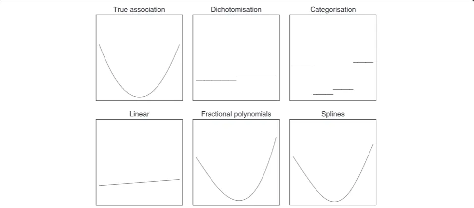
Below we outline various methods to adjust for continu-ous covariates, and highlight the assumptions made by each analysis. Figures 1 and 2 compare the estimated association for each method of analysis to the true association.
Dichotomisation
Dichotomisation involves splitting patients into two groups based on their covariate values. For example, pa-tients may be grouped according to their body mass index (BMI) score as either overweight (25 or over) or not overweight (under 25). As noted by others, this type of grouping can be helpful in clinical practice, but is not necessarily helpful for data analysis [29].
A dichotomised analysis can be implemented using the following model:
Y¼αþβTXTþβOXOþε
whereXTis a binary variable indicating whether the
pa-tient received treatment or control,βTis the effect of
whether the patient was overweight (BMI > 25),βOis the
effect of being overweight, andεis a random error term. The primary issue with dichotomisation is that it throws away a large amount of information, which can reduce power. For example, an analysis that treated BMI as continuous would recognise that BMI values of 24 and 26 are different, but much more similar to each other than BMI values of 16 or 34 are. However, a dichotomised analysis (grouped as less or more than 25) treats values of 16 and 24 as identical, values of 26 and
34 as identical, but treats BMI values of 24 and 26 as opposite.
Categorisation
Categorisation is when patients are grouped into mul-tiple categories. It is a generalisation of dichotomisa-tion; in this paper we assume categorisation involves three or more groups, in order to distinguish it from dichotomisation.
True association Dichotomisation Categorisation
Linear Fractional polynomials Splines
Fig. 1Estimated associations for different methods of analysis for y = log(x). *To obtain the estimated association between f(x) and y for each
method of analysis, we first generated a single data set from the model y = log(x) +ε(whereε~ N(0, 1). We then fit a linear regression model of the form y = f(x) to obtain the estimated association
True association Dichotomisation Categorisation
Linear Fractional polynomials Splines
Fig. 2Estimated associations for different methods of analysis for y = x2. *To obtain the estimated association between f(x) and y for each method of
analysis, we first generated a single data set from the model y = x2+ε(whereε~ N(0, 1). We then fit a linear regression model of the form y = f(x) to
Like dichotomisation, categorisation reduces the amount of information in the analysis, potentially leading to a loss in power. However, due to the increased number of categories, less information will be lost than in dichotomi-sation, and it should therefore give better results. For example, categorising BMI into underweight (<18.5), normal weight (18.5 to 24.9), overweight (25 to 29.9), or obese (30 or more) allows BMI scores of 16, 24, 26, and 30 to each have a different effect on outcome, un-like dichotomisation.
A categorised analysis can be implemented using the following model:
Y¼αþβTXTþβNXNþβOVXOV þβOBXOBþε
where XN, XOV, and XOBindicate whether the patient is
normal weight, overweight, or obese respectively, and
βN, βOV, and βOB are the effects of being in these BMI
categories compared to being underweight.
In general, a higher number of categories leads to less information lost [21]. However, having too many cat-egories can be problematic, particularly with a small sample size. This can lead to reduced power due to the extra parameters in the model [1]. It can also lead to in-flated type I error rates and biased estimates of treat-ment effect for binary or time-to-event outcomes when the number of categories is high compared to the num-ber of events [1].
Linear association
A linear analysis keeps the covariate as continuous, and assumes the association between covariate and outcome is linear. This analysis assumes the effect of an increase in the covariate is constant across the range of the co-variate. For example, an increase in BMI from 15 to 16 would have the same impact on outcome as an increase from 29 to 30.
A linear analysis can be implemented using the follow-ing model:
Y¼αþβTXTþβBMIXBMI þε
where XBMI represents BMI on a continuous scale, and βBMIrepresents the effect of a one-unit increase in BMI
on outcome.
The primary advantage of a linear analysis over cat-egorisation is that it makes full use of the data, and so should increase study power. However, if the true associ-ation between covariate and outcome is non-linear, then a linear analysis will be misspecified and may lead to re-ductions in power.
Fractional polynomials
Fractional polynomial models use polynomial trans-formations to estimate the association between the
covariate and outcome. They typically use either one or two polynomial terms. A model using only one polyno-mial term is referred to as an‘FP1’model, and a model using two polynomials terms an ‘FP2’ model. An FP1 can be written as follows:
Y¼αþβTXTþβ1XPBMI1 þε
wherep1is a polynomial transformation estimated from
the set {−2,−1,−0.5, 0, 0.5, 1, 2, 3} (wherep= 0 is taken to mean, by convention, log(X)).
A model with two polynomial terms (FP2) can be writ-ten as:
Y¼αþβTXTþβ1XBMIP1 þβ2XPBMI2 þε
where p1 and p2 are polynomial transformations
esti-mated from the set {−2,−1,−0.5, 0, 0.5, 1, 2, 3} (where
p= 0 corresponds to log(X)). By convention, p1=p2 is
taken to mean a model in which the two terms are
β1XBMI P1
andβ2XBMI P2
log(XBMI).
Either FP1 or FP2 models could be used in practice. It is possible to use the trial data to select between FP1 and FP2 models, however we do not recommend this approach, as covariate selection procedures have been shown to lead to poor results [30]. We therefore recom-mend pre-specifying the use of either an FP1 or FP2 model, and consider both approaches in this paper. Fur-thermore, in some software packages fractional polyno-mials also incorporate a model selection algorithm, where they drop covariates which are not prognostic enough (e.g. in the example above, they may drop BMI from the final model if it does not meet some pre-defined statistical significance threshold). As mentioned earlier, we do not recommend model selection in RCTs, and so for the purposes of this paper we have only con-sidered fractional polynomial models which include all covariates, regardless of their statistical significance.
The benefits of using a fractional polynomial approach include keeping the data as continuous, and allowing for non-linear associations. Fractional polynomials can be implemented in most standard statistical packages (e.g. using thefpormfpcommands in Stata, or themfp pack-age in R). Further details on fractional polynomials are available elsewhere [13, 31].
Restricted Cubic Splines
RCS is implemented by splitting the continuous cova-riate into separate sections, separated by m different knots, k1< k2<…< km. Within each of these sections, a
polynomial relationship between the covariate and out-come is estimated; these polynomial functions are joined up at the knots, to ensure a smooth curve across the range of the covariate. Two boundary knots kmin< k1
covariate) are also used; RCS estimates a linear associ-ation between covariate and outcome in these boundary knots, i.e. betweenkminandk1,and kmandkmax.
The model can be written as:
Y¼βTXTþS BMIð Þ þε
where
S BMIð Þ ¼γ0þγ1XBMIþ
Xm
j¼1
γj
h
XBMI−kj
3
þ
−λjðXBMI−kminÞ3þ− 1−λj
XBMI−kmax
ð Þ3
þ
i
and
XBMI−k
ð Þ3
þ¼
f
ðXBMI−kÞ3 if X
BMI≥k
0 if XBMI <k
and
λj¼
kmax−kj
kmax−kmin
Although seemingly complicated, RCS can easily be implemented in most software packages (e.g. the
mksplinecommand in Stata, the effectoption in SAS, or the hmisc package in R). In practice one must specify the number of knots to use, and where to place them. One could estimate the optimal number and location of the knots based on the trial data, but as above, these types of model selection procedures do not always work well for RCTs, and we therefore recommend that these choices are pre-specified. In this paper, we consider both 3 and 5 knots, and placing them at specified percentiles of the data [15].
RCSs have similar benefits to fractional polynomials: they keep the data as continuous, and allow for non-linear associations. Further details on RCSs are available elsewhere [15].
Simulation study
We performed a simulation study to compare different methods of accounting for a continuous covariate in the analysis of a RCT with both continuous and binary outcomes.
We generated outcomes from the following model:
Yi¼αþβTXTiþβcovf Xð Þ þi εi
whereXTi is a binary variable indicating whether the
pa-tient received treatment or control,βTis the effect of
re-ceiving treatment, Xi is a continuous covariate,f (.) is a
transformation,βcovis the effect of the transformed
co-variate, andεiis a random error term.
For continuous outcomes, we setεito follow a normal
distribution with mean 0 and standard deviationσe, with σeequal to 1.
For binary outcomes, we setεito follow a logistic
dis-tribution with mean 0 and variance π2/3. Yithen
repre-sents a latent continuous outcome, and a binary response was generated as 1 if Yi> 0 and 0 otherwise.
This model implies theβ’s represent log odds ratios. For both outcome types we assessed three scenarios forX:
A linear association with the outcome:f(X) =X
A non-linear, monotonic association with the
out-come:f(X) =eX
A non-linear, non-monotonic association with the
outcome:f(X) =X2
For each scenario we generated X from a normal dis-tribution with mean 0 and standard deviation 1.
We choseβcovbased on the following formula:
βcovðp90−p10Þ ¼σe
wherepzis thezthpercentile off(X); that is, an increase
from the 10th to the 90th percentile in f(X) would in-crease the outcome by one unit of σe. For continuous
outcomes, this led to βcov values of 0.385, 0.300, and
0.372 for linear, non-linear monotonic, and non-linear non-monotonic associations respectively. For binary out-comes, this led to βcovvalues of 0.700, 0.550, and 0.674
for linear, linear monotonic, and linear non-monotonic associations respectively.
We set the sample size to 200 patients for continuous outcomes, and to 600 for binary outcomes. These values were selected based on a review of trials published in high impact general medical journals which found these were the median sample sizes for trials with each out-come type [8]. Patients were randomised to one of two treatment arms using simple randomisation. For each simulation scenario (linear, monotonic, non-monotonic) we used two treatment effects: βT was set to 0, or βT
was set to give 80 % power based on the sample size (as-suming correct specification of the association between covariate and outcome). For binary outcomes we set the event rate in the control arm to 50 %.βTwas set to give
80 % power based on both the sample size and the effect ofβcovon outcome; because the effect ofβcovdiffered
ac-cording to the scenario, this implies that βT was set to
different values depending on the type of association be-tween covariate and outcome.
assuming a linear association; (d) using fractional poly-nomials, with one polynomial term (FP1); (e) using frac-tional polynomials, with two polynomial terms (FP2); (f ) using restricted cubic splines with 3 knots (knots were placed based on Harrell’s recommended percentiles [15]); and (g) using restricted cubic splines with 5 knots (knots were placed based on Harrell’s recommended percentiles [15]).
For each scenario we calculated the bias in the esti-mated treatment effect, the type I error rate (whenβT= 0)
and the power (whenβT≠0). For each simulation scenario
we used 5000 replications.
Re-analysis of MIST2 and APC trials
We applied the different methods of accounting for con-tinuous covariates to the MIST2 and advanced prostate cancer (APC) trials. MIST2 compared four treatments for patients with pleural infection [32]; placebo, tPA, DNase, or tPA + DNase. We focus on the treatment comparison between tPA + DNase vs. placebo for simpli-city. We used a logistic regression model to re-analyse the outcome of surgery at three months. Of the 192 pa-tients included in the analysis, 31 (16 %) experienced an event. We adjusted for the size of the patient’s pleural ef-fusion at baseline (continuous covariate), as well as two binary covariates: whether the infection was hospital ac-quired and whether the infection was purulent. All three covariates were minimisation factors. In our re-analysis, we handled the continuous covariate (size of the pa-tient’s pleural effusion) in eight different ways: (a) we ex-cluded it; (b) we dichotomised it at its sample median; (c) we categorised it at its sample 25th, 50th, and 75th percentiles; (d) we included it as a continuous covariate, assuming a linear association with outcome; (e) we used an FP1 model; (f ) we used an FP2 model; (g) we used
RCS with 3 knots; and (h) we used RCS with 5 knots. For the fractional polynomial models, we forced the model to include the covariate regardless of its signifi-cance level, and for the RCS models, we placed the knots at the percentiles recommended by Harrell.
The APC trial compared diethyl stilboestrol vs. placebo on overall survival in patients with advanced prostate can-cer. We used a Cox regression model to re-analyse the outcome of overall mortality. In our re-analysis we used the dataset supplied by Royston and Sauerbrei [13]. Of 475 patients included in the analysis, 338 (71 %) experi-enced an event. We adjusted for three continuous covari-ates: patient weight, tumour size, and stage grade. All three are prognostic factors associated with mortality. We used the same methods of analysis as for the MIST2 trial above. We analysed each of the three continuous covari-ates using the same method (that is, dichotomised all three, used an FP2 model for all three, etc.).
Results
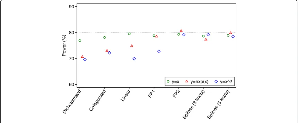
Simulation results for continuous outcomes
All methods of analysis provided unbiased estimates of treatment effect, and correct type I error rates (range 4.7 to 5.7 %) across all scenarios.
Results for power are shown in Fig. 3. For data gener-ated under a linear association, all methods of analysis which kept the covariate X as continuous (linear ana-lysis, fractional polynomials, and restricted cubic splines) had nominal power. Conversely, dichotomisation and categorisation led to small reductions in power.
For data generated under a non-linear, monotonic asso-ciation, FP and splines gave the highest power. A linear analysis led to a reduction in power of about 5.8 % com-pared to FP2, and dichotomisation and categorisation gave reductions of about 10.0 and 7.6 % respectively.
60 70 80 90
Power (%)
Dichotomised Categorised
Linear FP1 FP2
Splines (3 knots) Splines (5 knots)
y=x y=exp(x) y=x^2
For data generated under a non-linear, non-monotonic association, FP2 and splines with 3 or 5 knots gave the highest power. A linear analysis and dichotomisation had the lowest power (9.3 and 9.6 % reductions respect-ively vs. FP2), and categorisation lost 7.0 % power. The FP1 model lost 6.4 % power compared to FP2.
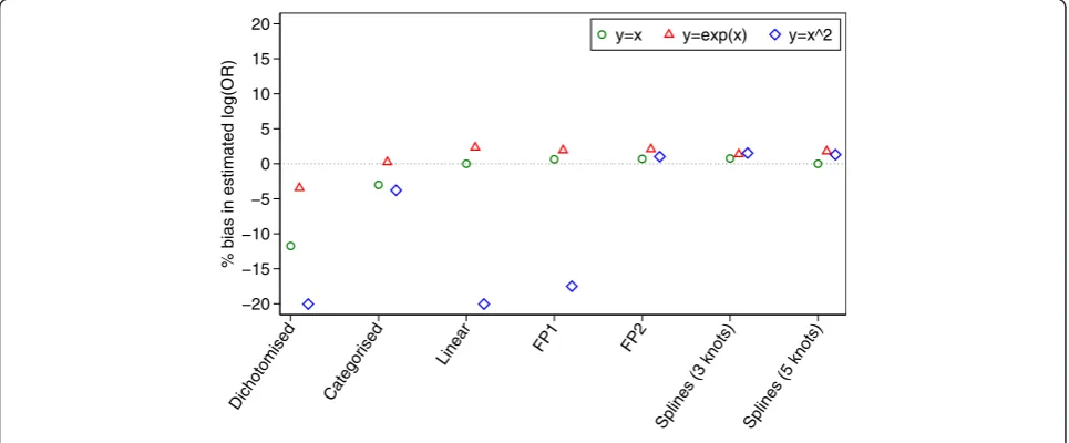
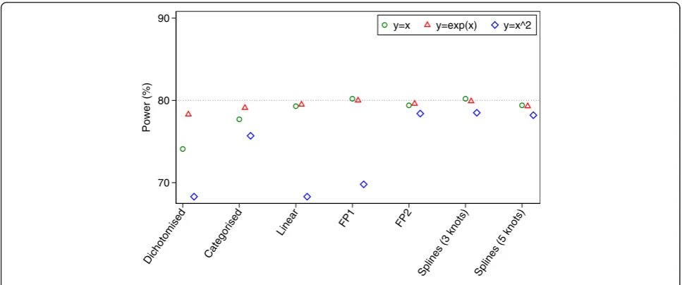
Simulation results for binary outcomes
Results are shown in Figs. 4 and 5. All methods of ana-lysis were unbiased when the treatment had no effect (i.e. when the odds ratio = 1), and gave correct type I error rates (range 4.6 to 5.7 %) across all scenarios. When the treatment was effective (i.e. when the odds ra-tio≠1), dichotomisation, categorisation, a linear analysis, and FP1 models all led to bias in certain scenarios. This was most pronounced for data generated under a non-linear, non-monotonic association; dichotomisation, a linear analysis, and FP1 all led to the log(OR) being biased downwards by around 20 %. Conversely, FP2 and splines with 3 or 5 knots all produced unbiased esti-mates across all scenarios. Results are shown in Fig. 4.
For data generated under a linear association, a linear analysis, FP, and splines all gave unbiased estimates of treatment effect and similar power. The log odds ratios for dichotomisation and categorisation were attenuated by 11.7 and 3.0 % respectively, leading to a reduction in power of 5.2 and 1.6 % compared to a linear analysis.
Under a non-linear monotonic association, a linear analysis, FP, and splines all gave unbiased estimates of treatment effect and nominal power. Dichotomisation and categorisation had very little attenuation in the es-timated treatment effects, and small reductions in power compared to FP (1.3 % dichotomisation, 0.5 % categorisation).
Under a non-linear, non-monotonic association, FP2 and splines with 3 or 5 knots gave unbiased treatment estimates and good power. Categorisation led to a small attenuation of the estimated log odds ratio, leading to a small decrease in power compared to FP2. A linear ana-lysis and dichotomisation both led to substantially atten-uated treatment effects, leading to large decreases in power compared to FP2 (9.1 % linear, 9.3 % dichotomi-sation). The FP1 model also led to a large degree of bias in the estimated treatment effect, and subsequently a large reduction in power (8.6 %) compared to FP2. This is because FP1 only allows for a monotone association betweenXandY.
Results of re-analysis of MIST2 and APC trials
Results can be found in Table 1. In both trials, un-adjusted/dichotomised/categorised analyses led to smaller treatment effect estimates than linear/FP/spline analyses. Treatment effect estimates were reduced by 35, 24, and 6 % for unadjusted, dichotomised, and cate-gorised analyses respectively, compared to FP or splines in MIST2. This attenuation in the estimated treatment effects led to larger p-values for unadjusted, dichoto-mised, and categorised analyses in most cases, which sometimes led to results becoming non-significant.
Discussion
Misspecification of the association between a continuous covariate and the outcome in RCTs can lead to substan-tial reductions in power. This occurs due to a reduction in the precision of the estimated treatment effect for linear analyses (such as continuous outcomes, or a dif-ference in proportions) and a reduction in the size of the estimated treatment effect for non-linear models (such as a binary or time-to-event outcome with censoring
−20 −15 −10 −5 0 5 10 15 20
% bias in estimated log(OR)
Dichotomised Categorised
Linear FP1 FP2
Splines (3 knots) Splines (5 knots)
y=x y=exp(x) y=x^2
estimated using an odds or hazard ratio). The extent to which results are affected is influenced by the extent of the misspecification.
Re-analysis of the MIST2 and APC trials found that omitting a covariate from the analysis led to larger at-tenuation of the estimated treatment effect compared to including the covariate, even if the association between covariate and outcome was misspecified. This is likely because excluding a covariate from the analysis can be seen as a more severe form of misspecification, and therefore resulted in larger losses in precision and attenu-ation of treatment effects. Therefore, we recommend adjusting for covariates even if the true association is unknown.
Our simulation study demonstrated that analyses which keep covariates as continuous generally perform better than analyses that use dichotomisation or categor-isation. The simplest method of keeping a covariate continuous is to assume a linear association with the outcome. A linear analysis will perform well if the asso-ciation between covariate and outcome is approximately
linear. However, there may be large reductions in power in the presence of departures from linearity. If non-linearity is possible, then FP2 models or splines are both suitable options, as they have been shown to increase power compared to alternative methods. FP1 models should be used with caution, as these provide very poor results under non-linear, non-monotonic associations. This is because FP requires all covariates to take only positive values, and therefore the outcome is a mono-tone function of the covariates for any FP1 model.
One issue to consider when deciding if a covariate is likely to have a linear association with outcome is the expected range of the covariate within the trial popula-tion. This range will often be smaller in trials than in ob-servational studies due to more restrictive inclusion/ exclusion criteria. Covariates with a non-linear associ-ation across their entire range may actually have a linear or approximately linear association across certain sub-sets of their range. For example, imagine BMI is non-linear across the range 16–35. Then, for any small portion of this range (e.g. 16–20, 20–24, etc.), the
70 80 90
Power (%)
Dichotomised Categorised
Linear FP1 FP2
Splines (3 knots) Splines (5 knots)
y=x y=exp(x) y=x^2
Fig. 5Simulation results for binary outcomes (power)
Table 1Results from different methods of adjusting for continuous covariates in APC and MIST2 trials
APC MIST2
Analysis methods HR (95 % CI) P-value OR (95 % CI) P-value
Unadjusted 0.84 (0.68 to 1.04) 0.11 0.23 (0.05 to 1.15) 0.07
Dichotomised 0.82 (0.66 to 1.01) 0.06 0.21 (0.04 to 1.07) 0.06
Categorised 0.82 (0.66 to 1.01) 0.07 0.18 (0.03 to 0.94) 0.04
Linear 0.79 (0.64 to 0.98) 0.03 0.16 (0.03 to 0.87) 0.03
FP1 0.79 (0.64 to 0.98) 0.03 0.17 (0.03 to 0.90) 0.04
FP2 0.78 (0.63 to 0.97) 0.03 0.17 (0.03 to 0.90) 0.04
Splines (3 knots) 0.80 (0.64 to 0.99) 0.04 0.18 (0.03 to 0.96) 0.04
association may be at least approximately linear. There-fore, in a trial recruiting only overweight patients (BMI 25–29.5), a linear analysis may be appropriate.
Continuous covariates are often categorised when used as stratification factors during randomisation. Stratifica-tion or minimisaStratifica-tion induces correlaStratifica-tion between treat-ment arms, and it is therefore necessary to account for this correlation in the analysis to obtain valid standard errors and type I error rates [8, 9]. In practice, this means we must include the stratification factors in our analysis. It is therefore of interest to know whether we must use the (categorised) stratification factor, or whether we can use the continuous version. Theoretic-ally, correctly modelling the functional form of the con-tinuous covariate in the analysis should adequately account for the correlation induced by the stratified ran-domisation procedure, and so this approach should lead to valid standard errors and type I error rates, as well as increased power. However, further research to confirm this hypothesis would be useful.
Both fractional polynomials and restricted cubic splines require certain decisions to be made about their implementation (e.g. FP1 or FP2, number and placement of knots, etc.), and in practice, we could use the trial data to make these choices. For example, one could esti-mate the optimal number and location of the knots. However, when using trial data to select the model, there is a risk of model overfitting, which can lead to poor re-sults. We therefore suggest that model selection be kept to a minimum, and that the form of the covariates be pre-specified [33, 34]. In addition to pre-specifying the general analysis approach (e.g. assuming a linear associ-ation vs. fractional polynomials vs. restricted cubic splines), it is necessary to pre-specify the implementa-tion of these approaches. For fracimplementa-tional polynomials, this entails pre-specifying the whether an FP1 or FP2 model will be used. For restricted cubic splines, this entails pre-specifying the number and location of the knots. We also note that both fractional polynomials and RCS can be combined with model selection algorithms which determine which covariates should be kept in the final model, and which covariates should be discarded (usu-ally based on a statistical significance threshold). How-ever, analysis methods which rely on p-values to determine the form of the final model have been shown to give poor results in RCTs in a variety of scenarios [30, 35–37], and so we do not recommend this approach. In-stead, we recommend when using fractional polynomials or splines that all covariates are included in the model regardless of their statistical significance.
Conclusion
We recommend (1) adjusting for continuous covariates even if their association with outcome is unknown; (2)
keeping covariates as continuous; and (3) using frac-tional polynomials with two polynomial terms or re-stricted cubic splines with between 3–5 knots when a linear association is in doubt.
Ethics approval and consent to participate
Not applicable.
Consent for publication
Not applicable.
Availability of data and materials
Data from the APC trial are available inRoyston P, Saur-brei W. Multivariable Model-Building. Chichester, Eng-land. : Wiley; 2008. The authors of this manuscript do not have permission to share data from the MIST2 trial.
Abbreviations
APC:Advanced prostate cancer; BMI: Body mass index; CPMP: Committee for
Proprietary Medicinal Products; FP: Fractional polynomial; MIST2: The second multicentre intrapleural sepsis trial; RCT: Randomised controlled trial; RCS: Restricted cubic splines.
Competing interests
The authors declare that they have no competing interests.
Authors’contributions
BK: concept, design of simulation study, conducted simulations, wrote manuscript. HR: design of simulation study, conducted simulations, contributed to manuscript. TM: design of simulation study, contributed to manuscript. RD: design of simulation study, contributed to manuscript. All authors read and approved the final manuscript.
Acknowledgements
We would like to thank the reviewer for helpful comments on the manuscript.
Funding
No authors received specific funding for this work. Tim Morris is funded by the MRC London Hub for Trials Methodology Research, grant MC_EX_G0800814.
Author details
1Pragmatic Clinical Trials Unit, Queen Mary University of London, London, UK. 2University of Manchester, Manchester, UK.3MRC Clinical Trials Unit at UCL,
London School of Hygiene and Tropical Medicine, London, UK.4Medical Statistics Department, London School of Hygiene and Tropical Medicine, London, UK.
Received: 9 September 2015 Accepted: 1 April 2016
References
1. Kahan BC, Jairath V, Dore CJ, Morris TP. The risks and rewards of covariate adjustment in randomized trials: an assessment of 12 outcomes from 8 studies. Trials. 2014;15:139.
2. Hernandez AV, Eijkemans MJ, Steyerberg EW. Randomized controlled trials with time-to-event outcomes: how much does prespecified covariate adjustment increase power? Ann Epidemiol. 2006;16(1):41–8. 3. Hernandez AV, Steyerberg EW, Habbema JD. Covariate adjustment in
randomized controlled trials with dichotomous outcomes increases statistical power and reduces sample size requirements. J Clin Epidemiol. 2004;57(5):454–60.
5. Turner EL, Perel P, Clayton T, Edwards P, Hernandez AV, Roberts I, et al. Covariate adjustment increased power in randomized controlled trials: an example in traumatic brain injury. J Clin Epidemiol. 2012;65(5):474–81.
6. Thompson DD, Lingsma HF, Whiteley WN, Murray GD, Steyerberg EW.
Covariate adjustment had similar benefits in small and large randomized controlled trials. J Clin Epidemiol. 2015;68(9):1068–75.
7. Nicholas K, Yeatts SD, Zhao W, Ciolino J, Borg K, Durkalski V. The impact of covariate adjustment at randomization and analysis for binary outcomes: understanding differences between superiority and noninferiority trials. Stat Med. 2015;34(11):1834–40.
8. Kahan BC, Morris TP. Reporting and analysis of trials using stratified randomisation in leading medical journals: review and reanalysis. BMJ. 2012; 345:e5840.
9. Kahan BC, Morris TP. Improper analysis of trials randomised using stratified blocks or minimisation. Stat Med. 2012;31(4):328–40.
10. Kahan BC, Morris TP. Adjusting for multiple prognostic factors in the analysis of randomised trials. BMC Med Res Methodol. 2013;13:99.
11. Kahan BC, Morris TP. Assessing potential sources of clustering in individually randomised trials. BMC Med Res Methodol. 2013;13:58.
12. Parzen M, Lipsitz S, Dear K. Does clustering affect the usual test statistics of no treatment effect in a randomized clinical trial? Biom J. 1998;40(4):385–402. 13. Royston P, Saurbrei W. Multivariable Model-Building. Chichester: Wiley; 2008. 14. Durrleman S, Simon R. Flexible regression models with cubic splines. Stat
Med. 1989;8(5):551–61.
15. Harrell Jr FE. Regression modeling strategies: with applications to linear models, logistic regression, and survival analysis. New York: Springer; 2001. 16. Brenner H, Blettner M. Controlling for continuous confounders in
epidemiologic research. Epidemiology (Cambridge, Mass). 1997;8(4):429–34. 17. MacCallum RC, Zhang S, Preacher KJ, Rucker DD. On the practice of
dichotomization of quantitative variables. Psychol Methods. 2002;7(1):19–40. 18. Royston P, Altman DG, Sauerbrei W. Dichotomizing continuous predictors in
multiple regression: a bad idea. Stat Med. 2006;25(1):127–41. 19. Sauerbrei W, Royston P, Binder H. Selection of important variables and
determination of functional form for continuous predictors in multivariable model building. Stat Med. 2007;26(30):5512–28.
20. Committee for Proprietary Medicinal Products (CPMP). Points to consider on adjustment for baseline covariates. Stat Med. 2004;23(5):701–9.
21. Schmoor C, Schumacher M. Effects of covariate omission and categorization when analysing randomized trials with the Cox model. Stat Med. 1997;16(1–3): 225–37.
22. Berger VW. Valid adjustment of randomized comparisons for binary covariates. Biom J. 2004;46(5):589–94.
23. Rosenbaum PR. The Consequences of Adjustment for a Concomitant
Variable That Has Been Affected by the Treatment. J Roy Stat Soc a Sta. 1984;147:656–66.
24. Rosenberger WF, Lachin JM. Randomization in Clinical Trials. New York: John Wiley & Sons, Inc.; 2005.
25. Yang L, Tsiatis A. Efficiency Study of Estimators for a Treatment Effect in a Pretest-Posttest Trial. The American Statistician. 2001;55(4):314–21. 26. Gail M, Wieand S, Piantadosi S. Biased estimates of treatment effect in
randomized experiments with nonlinear regressions and omitted covariates. Biometrika. 1984;71(3):431–44.
27. Hauck WW, Anderson S, Marcus SM. Should we adjust for covariates in nonlinear regression analyses of randomized trials? Control Clin Trials. 1998; 19(3):249–56.
28. Robinson LD, Jewell NP. Some surprising results about covariate adjustment in logistic regression models. Int Stat Rev. 1991;58:227–40.
29. Altman DG, Royston P. The cost of dichotomising continuous variables. BMJ. 2006;332(7549):1080.
30. Raab GM, Day S, Sales J. How to select covariates to include in the analysis of a clinical trial. Control Clin Trials. 2000;21(4):330–42.
31. Morris TP, White IR, Carpenter JR, Stanworth SJ, Royston P. Combining fractional polynomial model building with multiple imputation. Stat Med. 2015;34(25):3298–317.
32. Rahman NM, Maskell NA, West A, Teoh R, Arnold A, Mackinlay C, et al. Intrapleural use of tissue plasminogen activator and DNase in pleural infection. N Engl J Med. 2011;365(6):518–26.
33. Kahan BC, Jairath V, Murphy MF, Dore CJ. Update on the transfusion in gastrointestinal bleeding (TRIGGER) trial: statistical analysis plan for a cluster-randomised feasibility trial. Trials. 2013;14:206.
34. Chan AW, Tetzlaff JM, Gotzsche PC, Altman DG, Mann H, Berlin JA, et al. SPIRIT 2013 explanation and elaboration: guidance for protocols of clinical trials. BMJ. 2013;346:e7586.
35. Freeman PR. The performance of the two-stage analysis of two-treatment, two-period crossover trials. Stat Med. 1989;8(12):1421–32.
36. Kahan BC. Bias in randomised factorial trials. Stat Med. 2013;32(26):4540–9. 37. Shuster JJ. Diagnostics for assumptions in moderate to large simple clinical
trials: do they really help? Stat Med. 2005;24(16):2431–8.
• We accept pre-submission inquiries
• Our selector tool helps you to find the most relevant journal
• We provide round the clock customer support • Convenient online submission
• Thorough peer review
• Inclusion in PubMed and all major indexing services
• Maximum visibility for your research
Submit your manuscript at www.biomedcentral.com/submit