Solving the OSCAR and SLOPE Models Using a
Semismooth Newton-Based Augmented Lagrangian Method
Ziyan Luo [email protected]
Department of Mathematics Beijing Jiaotong University Beijing, P. R. China
Defeng Sun [email protected]
Department of Applied Mathematics The Hong Kong Polytechnic University Hong Kong
Kim-Chuan Toh [email protected]
Department of Mathematics, and Institute of Operations Research and Analytics National University of Singapore
Singapore
Naihua Xiu [email protected]
Department of Mathematics Beijing Jiaotong University Beijing, P. R. China
Editor:Benjamin Recht
Abstract
The octagonal shrinkage and clustering algorithm for regression (OSCAR), equipped with the `1-norm and a pair-wise `∞-norm regularizer, is a useful tool for feature selection
and grouping in high-dimensional data analysis. The computational challenge posed by OSCAR, for high dimensional and/or large sample size data, has not yet been well resolved due to the non-smoothness and non-separability of the regularizer involved. In this paper, we successfully resolve this numerical challenge by proposing a sparse semismooth Newton-based augmented Lagrangian method to solve the more general SLOPE (the sorted L-one penalized estimation) model. By appropriately exploiting the inherent sparse and low-rank property of the generalized Jacobian of the semismooth Newton system in the augmented Lagrangian subproblem, we show how the computational complexity can be substantially reduced. Our algorithm offers a notable computational advantage in the high-dimensional statistical regression settings. Numerical experiments are conducted on real data sets, and the results demonstrate that our algorithm is far superior, in both speed and robustness, to the existing state-of-the-art algorithms based on first-order iterative schemes, including the widely used accelerated proximal gradient (APG) method and the alternating direction method of multipliers (ADMM).
Keywords: Linear Regression, OSCAR, Sparsity, Augmented Lagrangian Method, Semi-smooth Newton method
c
1. Introduction
Feature selection and grouping is highly beneficial in learning with high-dimensional data containing spurious features, and thus has found wide applications in statistics (Hocking, 1976; Miller, 2002), computer vision (Mairal et al., 2014), signal processing (Chen et al., 1998; Tropp, 2006; Figueiredo et al., 2007), bioinformatics (Wang et al., 2005; Rapaport et al., 2007). The octagonal shrinkage and clustering algorithm for regression (OSCAR) proposed by (Bondell and Reich, 2008), serves as an efficient sparse modeling tool with automatic feature grouping by employing the`1-norm regularizer together with a pairwise `∞penalty. The OSCAR penalized problem for linear regression with the least squares loss
function takes the form of
min
x∈Rn
1
2kAx−bk
2+w1kxk 1+w2
X
i<j
max{|xi|,|xj|}, (1)
where b∈Rm is the response vector,A∈
Rm×n is the design matrix,x ∈Rn is the vector
of unknown coefficients to be estimated,w1 and w2 are two nonnegative tuning parameters
for the tradeoff of the sparsity and equality of coefficients for correlated features promoted by the `1-norm and the pairwise `∞ term, respectively. Note that in high dimensional
statistical regressions, we often have n m, that is, the number of features is larger than the sample size.
The OSCAR penalized problem (1) is a convex optimization problem. When the pair-wise `∞ term is removed, the problem (1) is reduced to the well-known LASSO model
proposed by Tibshirani (1996) in statistics and a rich variety of algorithms have been pro-posed, most of them have taken the advantage of the componentwise separability of the
`1-norm in their algorithmic design. With the additional pairwise`∞ term, the problem (1)
becomes understandably more challenging due to the lack of separability of the OSCAR reg-ularization term. In Bondell and Reich (2008), the traditional quadratic programming (QP) and sequential quadratic programming (SQP) based algorithms are employed for solving (1) with numerical implementations limited to small data sets. Efficient numerical algorithms are in dire need especially for large scale problems resulting from the explosion in the size and complexity of modern data sets in practical applications. In Zhong and Kwok (2012), the accelerated proximal gradient (APG) method, proposed by Nesterov (1983) and coined as FISTA for the `1-norm regularization problem by Beck and Teboulle (2009), is adopted for solving relatively large scale instances by taking advantage of the efficient computation of the proximal mapping of the OSCAR penalty function, which is explained in the next paragraph.
We begin by introducing some notation. For a given vector x ∈ Rn, denote |x| to be
the vector obtained fromxby taking the absolute value of its components. Let|x|(i) be the
i-th largest component of|x|such that|x|(1)≥ |x|(2)· · · ≥ |x|(n). With the above notation, the OSCAR penalty can be written as
w1kxk1+w2
n
X
i=1
max
i<j {|xi|,|xj|} = n
X
i=1
λi|x|(i), (2)
whereλi =w1+w2(n−i), i= 1, . . . , n, satisfy the property that λ1 ≥λ2 ≥ · · · ≥λn ≥0.
The resulting regularization function κλ(x) :=
Pn
decreasing weighted sorted `1-norm (DWSL1) by Zeng and Figueiredo (2014b), is exactly
the weighted Ky Fan norm as studied in Wu et al. (2014) as long asλ1>0. The computation of the proximal mapping of DWSL1 has been studied in the literature (see, e.g., Zeng and Figueiredo, 2014a,b; Bogdan et al., 2015). It is heavily related to the pool adjacent violators algorithm (PAVA) for solving isotonic regression problems (Barlow and Brunk, 1972) in the field of ordered statistics (see, e.g., Robertson et al., 1988; Silvapulle and Sen, 2011).
As a more general framework of the OSCAR problem (1), the least-squares problem with the DWSL1 regularization term is called the sorted L-one penalized estimation (SLOPE), which has been shown to have good performance for controlling the false discovery rate (FDR) in sparse statistical models in Bogdan et al. (2015). The APG method is employed in the latter paper for solving the SLOPE model by relying on the efficient numerical evaluation of the proximal mapping of the sorted `1-norm. As can be seen, most of the existing methods for solving the OSCAR model and the more general SLOPE model in the large scale settings are based on the first-order information of the underlying nonsmooth optimization model. However, as demonstrated by the works of Li et al. (2018a) for the LASSO and Li et al. (2018b) for the fused LASSO, there are compelling evidences to suggest that one can design a much more efficient algorithm if one can fully exploit the inherent second-order sparsity and low-rank property present in the OSCAR model or the more general SLOPE model. In this paper, we will show how this can be achieved by focusing on the following SLOPE model:
min
x∈Rn
1
2kAx−bk
2+
n
X
i=1
λi|x|(i) (3)
with parametersλ1 ≥λ2 ≥ · · · ≥λn≥0 andλ1 >0. Note that here the parameter vector λ is a general vector satisfying the previous condition. It needs not be restricted to the parameter vector associated with the OSCAR penalty in (2).
The main goal of this paper is to design a semismooth Newton-based augmented La-grangian method (Newt-ALM for short) for solving the SLOPE model (2) from the dual perspective. As a main contribution of this paper, in Section 2 and Subsection 3.4, we will see that one can extract some special low-rank and sparsity structures in the gen-eralized Jacobian of the proximal mapping associated with the sorted `1-norm. In turn,
the Hessian matrices involved in the ALM subproblems also inherit the special structures which we can wisely exploit to design a very efficient semismooth Newton method to solve the subproblems. The latter fact, combined with the fast linear convergence of the aug-mented Lagrangian method which we will establish in Section 3, will enable our Newt-ALM algorithm to perform highly efficiently later in the numerical experiments on large scale instances. The comparison of our algorithm with the inexact ADMM (iADMM) proposed in Chen et al. (2017) and the APG method implemeneted in the SLOPE solver in Bogdan et al. (2015) for solving OSCAR problems indicates that our Newt-ALM can outperform these state-of-the-art first-order algorithms substantially.
addition, we also extract the low-rank and sparsity structures present in the generalized Jacobians of the proximal mapping of the sorted `1-norm. These structures are crucial for the efficient numerical computation in the semismooth Newton method. Numerical results are reported in Section 4 to demonstrate the high efficiency and robustness of our algorithm. We conclude our paper in Section 5. Technical proofs are provided in Appendix A.
2. The generalized Jacobian of the proximal mapping of the DWSL1 norm
As mentioned in the introduction, a key factor contributing to the high computational efficiency of our proposed Newt-ALM is the characterization of the generalized Jacobian matrix of the proximal mapping for the DWSL1 norm (or sorted `1-norm). In particular,
the characterization will enable us to extract the underlying low-rank and sparsity structures present in the generalized Jacobian which we can fully exploit for computational efficiency within the semismooth Newton method for solving the subproblem in each iteration of the augmented Lagrangian method. The purpose of this section is to present the characteri-zation of the generalized Jacobain of the proximal mapping for the DWSL1 norm and its analytical properties.
Let Πs
n be the set of all signed permutation matrices in Rn×n. Recall that an n×n
signed permutation matrix is a matrix whose rows are the permutation of those of then×n
identity matrix and the only non-zero element in each row can take the value ±1. Note that the cardinality ofΠs
n is 2nn!. For any given vector y∈Rn, denote
Πs(y) :=π∈Πsn|(πy)i =|y|(i), i= 1, . . . , n .
Letκλ(x) :=Pni=1λi|x|(i) withλ1 ≥ · · · ≥λn≥0. The proximal mapping ofκλ is
Proxκλ(y) = arg minx
1
2kx−yk
2+κ
λ(x)
, ∀y∈Rn.
Since the involved objective function is strongly convex (see, e.g., Wu et al., 2014; Bogdan et al., 2015) and piecewise quadratic, the proximal mapping Proxκλ is then piecewise affine,
a result known from Sun (1986) or (Rockafellar and Wets, 1998, Proposition 12.30). Define
xλ(w) := arg min x
1
2kx−wk
2+λ>x|Bx≥0
, w∈ <n, (4)
where
Bx= [x1−x2, x2−x3, . . . , xn−1−xn, xn]>∈Rn.
It is known from (Bogdan et al., 2015, Proposition 2.2) that for anyy∈Rn andπ ∈Πs(y),
Proxκλ(πy) = xλ(πy). Furthermore, for any λ ∈ R
n
+ satisfying λ1 ≥ · · · ≥ λn, and any
vectory∈Rn, we have
Proxκλ(y) =π −1x
λ(πy), ∀π∈Πs(y)⊆Πsn. (5)
Given the structure of xλ(·), one can see that the Jacobian of xλ(·) at any w∈ Rn, as
constructed in (Han and Sun, 1997), is given by
P(w) =
P ∈Rn×n|P =I−B>Γ
BΓBΓ> −1
BΓ,Γ∈ K(w)
Here
K(w) :={Γ⊆ {1, . . . , n} |Supp(zλ(w))⊆Γ⊆I(xλ(w))},
where zλ(w) = (BB>)−1B(w−λ−xλ(w)) is an optimal dual multiplier vector associated
with the inequality constraints in (4), I(xλ(w)) ={i∈ {1, . . . , n} | (Bxλ(w))i = 0} is the
set of active indices (the indices of the active constraints) in (4), andBΓ is the submatrix
obtained by extracting the rows of B with indices in Γ. In the above, Supp(zλ(w)) is the
support ofzλ(w), i.e., the index set of nonzero compomonents ofzλ(w). Observe that each
element ofP(w) is the projection onto the null space ofBΓfor some index set Γ sandwiched
between the set of active indices I(xλ(w)) and Supp(zλ(w)).
It is known from Lemma 2.1 in Han and Sun (1997) that for any w∈Rn, there exists
a neighborhoodW ofw such that for allw0 ∈W,
K(w0)⊆ K(w),
P(w0)⊆ P(w),
xλ(w0)−xλ(w)−P(w0−w) = 0, ∀P ∈ P(w0).
(7)
Define the multifunction M:Rn⇒Rn×n by
M(y) :=
M ∈Rn×n|M =π−1P π, π∈Πs(y), P ∈ P(πy) . (8) Recall that the set-valued mapping M : <n ⇒ <n×n is said to be upper
semicontin-uous (Aubin and Frankowska, 1990, Definition 1.4.1) at a certain point y ∈ <n if for any
neighborhood N of M(y), there exists a constantρ >0 such that
M(y0)⊂ N, ∀y0 ∈B(y, ρ) :=
y0 ∈ <n| ky0−yk ≤ρ .
Then we have the following theorem which is adapted from (Li et al., 2018b, Proposition 7). Its proof is given in Appendix A.
Theorem 1 Let λ ∈ Rn
+ be such that λ1 ≥ λ2 ≥ · · · ≥ λn. Then M(·) is a nonempty and compact valued, upper semicontinuous multifunction, and for any given y∈Rn, every M ∈ M(y) is symmetric and positive semidefinite. Moreover, there exists a neighborhood
U of y such that for all y0 ∈U,
Proxκλ(y
0)−Prox
κλ(y)−M(y
0−y) = 0, ∀M ∈ M(y0). (9)
Example. Next, we present an example to illustrate the result in equation (9) of Theorem 1 explicitly. Consider the vector y = [4,3,0]> and the parameter vector λ = [3,1,1]>. For any y0 = [y01, y20, y03]> that is sufficiently close to y, sayky0−yk ≤0.1, we can show by using the pool adjacent violators algorithm that
Proxκλ(y) =
1.5 1.5 0
, Proxκλ(y 0) =
y01+y20−4 2
y01+y20−4 2 0 . Thus
Proxκλ(y 0
)−Proxκλ(y) =M(y 0−
y) with M =
1/2 1/2 0 1/2 1/2 0 0 0 0
In this caseM(y0) ={M}.
Next, we discuss the semismoothness property of the proximal mapping Proxκλ. Recall
from Mifflin (1977); Kummer (1988); Qi and Sun (1993); Sun and Sun (2002) or directly from (Li et al., 2018b, Definition 1) that the semismoothness with respect to a given nonempty compact valued, upper semicontinuous multifunction is defined as follows.
Let O ⊆ Rn be any given open set, K : O ⇒
Rm×n be a nonempty compact valued,
upper semicontinuous multifunction, and F : O → Rm be a locally Lipschitz continuous
function, i.e., for any x ∈ O, there exist positive constants Lx and δx such that for all
y, y0 ∈ O satisfying ky−xk ≤δx and ky0−xk ≤δx, we get kF(y)−F(y0)k ≤Lxky−y0k. F
is said to besemismooth atx∈ O with respect to the multifunction K ifF is directionally differentiable atx and for any V ∈ K(x+d) withd→0,
F(x+d)−F(x)−V d=o(kdk).
Letγ be a positive scalar. F is said to beγ-order semismooth (stongly semismooth ifγ = 1) atx∈ O with respect toK ifF is directionally differentiable atxand for anyV ∈ K(x+d) withd→0,
F(x+d)−F(x)−V d=O(kdk1+γ).
F is said to be a semismooth (γ-order semismooth, stongly) function on O with respect toK ifF is semismooth (γ-order semismooth, strongly semismooth) everywhere inO with respect to K. It is known from Theorem 1 that Proxκλ is γ-order semismooth on R
n with
respect toMfor any given positiveγ.
3. A semismooth Newton augmented Lagrangian method
3.1. The algorithmic framework
GivenA∈Rm×n,b∈
Rm andλ1 ≥ · · · ≥λn≥0 withλ1 >0, the DWSL1 regularized least
squares problem can be rewritten as
(P) max
x∈Rn
−f(x) :=−1
2kAx−bk
2−κ
λ(x)
. (10)
Its dual problem takes the form of
(D) min
y∈Rm, ξ∈
Rn
1 2kyk
2+hb, yi+κ∗
λ(ξ)
A
>
y+ξ = 0
, (11)
where κ∗λ(v) := supx∈Rn{hx, vi −κλ(x)} is the Fenchel conjugate function of κλ. For any
given scalar σ > 0, the corresponding reduced augmented Lagrangian function associated with (D) is defined by
Lσ(y;x) := inf ξ∈Rn
1 2kyk
2+hb, yi+κ∗
λ(ξ)− hA
>
y+ξ, xi+σ 2kA
>
y+ξk2
= 1 2kyk
2+hb, yi+ inf
ξ∈Rn
κ∗λ(ξ) +σ 2kA
>
y+ξ−σ−1xk2− 1
2σkxk 2
= 1 2kyk
2+hb, yi − 1
2σkxk 2+σφ
κ∗
λ/σ
σ−1x−A>y
whereφκ∗
λ/σ is the Moreau-Yosida regularization ofκ ∗
λ/σ defined as
φκ∗
λ/σ(x) := minu∈
Rn
1
σκ ∗
λ(u) +
1
2ku−xk
2
, ∀x∈Rn.
The inexact augmented Lagrangian method (Rockafellar, 1976b) together with the semis-mooth Newton method will be employed to solve (D) with the algorithmic framework as described in Algorithm 1. Note that the most expensive part in each iteration of the ALM is in solving the subproblem in Step 1.
Algorithm 1:An inexact augmented Lagrangian method for (D) (Newt-ALM) Choose σ0>0 and y0, x0∈Rm×Rn . Fork= 0,1, . . ., perform the following steps
in each iteration:
Step 1. Compute yk+1≈arg min
y∈Rm
Ψk(y) :=Lσk(y;x
k) ;
Step 2. Compute xk+1= Proxσkκλ x
k−σ
kA>yk+1
;
Step 3. Update σk+1↑σ∞≤ ∞.
The stopping criteria for the approximation in Step 1 of the inexact augmented La-grangian method have been well discussed in Rockafellar (1976b,a). Given two summable sequences of nonnegative numbers, {k}k≥0 and {δk}k≥0, and a nonnegative convergent
sequence{δ0k}k≥0 with limit 0, the stopping criteria can be simplified as follows in our case:
(A) k∇Ψk(yk+1)k ≤k/
√
σk;
(B1) k∇Ψk(yk+1)k ≤(δk/
√
σk)kxk+1−xkk;
(B2) k∇Ψk(yk+1)k ≤(δk0/σk)kxk+1−xkk.
3.2. Convergence theory
The piecewise linear-quadratic property of f as defined in (10) leads to the polyhedral multifunction ∂f (the sub-differential off). By a fundamental result in Robinson (1981), this further implies that∂fsatisfies the error bound condition with a common modulus, say
af. Specifically, the error bound condition states that for the optimal solution set (∂f)−1(0)
of (P), which we denote by S∗, there exists someε >0 such that for any x∈Rn satisfying
dist(0, ∂f(x))≤ε, it holds that
dist(x, S∗)≤af dist(0, ∂f(x)). (12)
Similarly, consider the Lagrangian function associated with (D) which is defined by
l(y;x) := 1 2kyk
2+hb, yi+κ∗
λ(ξ)− hA>y+ξ, xi.
For the polyhedral multifunction Tl defined as Tl(y, x) = {(y0, x0) | (y0,−x0) ∈ ∂l(y;x)},
there exist somealandε0 >0 such that for any (y, x)∈Rm×Rnsatisfying dist(0, Tl(y, x))≤
ε0, it has
where y∗ is the unique optimal solution of (D). Following the results on global and local convergence of the ALM as stated in (Rockafellar, 1976b,a; Li et al., 2018a,b), we can readily obtain the following convergence results on Algorithm 1 with the above stopping criteria. As the proofs of the theorems are almost the same as those appeared in (Li et al., 2018a, Theorems 3.2 and 3.3), we will omit them here.
Theorem 2 (Global convergence) Let (yk, xk) be the infinite sequence generated by Algorithm 1 with stopping criterion (A) applied to Ψk in Step 1. Then
xk converges to an optimal solution to (P), and yk converges to the unique optimal solution of (D).
Theorem 3 (Local linear-rate convergence) Let(yk, xk) be the infinite sequence gen-erated by Algorithm 1 with stopping criteria (A) and (B1) applied to Ψk in Step 1. Then for all ksufficiently large,
distxk+1, S∗≤θkdist
xk, S∗,
where
θk:=
af
q a2
f +σk2
+ 2δk
1 1−δk
→ θ∞:=
af
q a2
f+σ∞2 <1
as k→ +∞, and af is from (12). Additionally, if the criterion (B2) is also adopted, then for all ksufficiently large,
kyk+1−y∗k ≤θk0kxk+1−xkk,
where
θ0k:= al(1 +δ
0
k)
σk
→ al
σ∞
as k→+∞, and al is from (13).
Remark 4 (Global linear-rate convergence) Besides the local linear-rate convergence as stated in Theorem 3, one can also obtain the global Q-linear convergence of the primal sequence {xk} and the global R-linear convergence of the dual infeasibility and the duality gaps for the sequence generated by Algorithm 1 based on (Cui et al., 2018, Proposition 2 and Lemma 3) or by mimicking the proofs of (Zhang et al., 2018, Theorem 4.1 and Remark 4.1) since problem (P) possesses the following property: For any positive scalar r, there exists t >0 such that
dist(x, S∗)≤tdist(0, ∂f(x)), ∀x∈Rn satisfying dist(x, S∗)≤r,
(see, Zhang et al., 2018, Proposition 2.2). We omit the details here.
3.3. The semismooth Newton method for solving the subproblem in Step 1
It is known from Moreau (1965) or (Rockafellar, 1970, Theorem 31.5) that Ψkis continuously
differentiable and
∇Ψk(y) =y+b−AProxσkκλ(x
k−σ
Since Ψkis strongly convex with bounded level sets, the unique solution of the minimization
subproblem, miny∈RmΨk(y), in Step 1 of the ALM can be computed by solving the following
first-order optimality condition
∇Ψk(y) = 0. (14)
For anyy∈Rm, define
Gk(y) :=nV ∈Rm×m |V =I
m+σkAM A>, M ∈ M
(σk)−1xk−A>y
o ,
whereMis defined in (8). The following semismooth Newton (SSN) method is then applied to solve the semismooth equation (14), as presented in Algorithm 2.
Algorithm 2:A semismooth Newton method for solving (14)
Choose µ∈(0,1/2), ¯η∈(0,1), δ∈(0,1),τ ∈(0,1], y0 ∈Rm. Forj = 0,1, . . .,
perform the following steps in each iteration:
Step 1. (Computing the Newton direction) Choose an element
Mj ∈ M((σk)−1xk−A>yj) and setVj :=Im+σkAMjA>. Solve the Newton
equation
Vjd=−∇Ψk(yj) (15)
exactly or by the conjugate gradient (CG) algorithm to get dj such that
kVjdj+∇Ψk(yj)k ≤min{η,¯ k∇Ψk(yj)k1+τ}.
Step 2. (Line search) Set αj =δmj, where mj is the least nonnegative integerm
satisfying
Ψk(yj +δmdj)≤Ψk(yj) +µδmh∇Ψk(yj), dji.
Step 3. Set yj+1 =yj +αjdj.
3.4. Efficient implementations of the semismooth Newton method
In this subsection, the sparsity and low-rank structure of the coefficient matrix in the linear system (15) will first be uncovered. Then the structures will be exploited through designing novel numerical techniques for solving the large scale system (15) to achieve efficient implementations of the semismooth Newton method in Algorithm 2. For any given index set Γ⊆ {1, . . . , n}, define the diagonal matrix ΣΓ ∈Rn×n by
(ΣΓ)ii=
1, ifi∈Γ; 0, otherwise.
Similar to the case in (Li et al., 2018b, Proposition 6), there exists some positive integerN
such that ΣΓ can be rewritten as a block diagonal matrix
ΣΓ = Diag(Λ1, . . . ,ΛN)
with Λi∈ {Oni, Ini} for eachi∈ {1, . . . , N}where any two consecutive blocks Λi and Λi+1
are not of the same type. Note thatOni denotes theni by ni zero matrix. Denote
Then we have
P =In−BΓ>(BΓBΓ>) −1B
Γ= Diag(P1, . . . , PN),
where
Pi =
1
ni+1eni+1e >
ni+1, ifi∈J and i6=N; Oni, ifi∈J and i=N; Ini−1, ifi /∈J and i6= 1; Ini, ifi /∈J and i= 1
with the convention I0 = ∅. This block diagonal matrix P can be further decomposed into the sum of a sparse diagonal term and a low-rank term as P = H +U UT, where
H= Diag(H1, . . . , HN)∈Rn×n with
Hi =
Oni+1, ifi∈J and i6=N;
Oni, ifi∈J and i=N; Ini−1, ifi /∈J and i6= 1; Ini, ifi /∈J and i= 1
and U ∈Rn×N with its (k, j)-th entry given by
Ukj =
1/p
nj+ 1, if j−1
P
t=1
nt+ 1≤k≤ j
P
t=1
nt+ 1 and j∈J\{N};
0, otherwise.
Define α:={j ∈ {1, . . . , n} |Hii= 1}={1, . . . , n}\Γ, and let UJN be the submatrix of U generated by extracting its columns indexed by J\{N}. Then for any givenA∈Rm×n,
any Γ ∈ {1, . . . , n} with its corresponding matrix P defined as above, and any signed permutation matrix π, we have
Aπ>P πA> = Aπ>HπA>+Aπ>U U>πA>
= Aπ(α,:)>π(α,:)A>+AeUeJNUeJ> NAe
>
=: V1V1>+V2V2>, (16)
where V1 = Aπ(α,:)>, V2 = AeUeJN with UeJN being the submatrix of UJN obtained by
dropping all its zero rows andAeis the submatrix obtained from the permuted matrixAπ>
by dropping the columns corresponding to those zero rows in UJN. We call the structure
uncovered in (16) that is inherited from the sparse plus low-rank structure of the generalized JacobianP as thesecond-order sparsity.
Based on the structure in (16), the cost of computingAπ>P πA>is dramatically reduced fromO(mn(n+m)) by naive computation toO(m2(r1+r2)), wherer1 is number of columns
in V1 and r2 is the number of columns in V2. Here r1 refers to the number of inactive
constraints inBx≥0, andr2 refers to the number of distinct nonzero identical components in Bx, both of which are generally no larger than the number of nonzero components of
x. In the setting of high-dimensional sparse grouping linear regression models, m, r1, r2
Ifmis not too large, we can use the (sparse) Cholesky factorization to directly solve the linear system (15). In the case where r1+r2 m, the cost of solving (15) can be further reduced by using the Sherman-Morrison-Woodbury (SMW) formula as follows:
Im+σAπ>P πA>
−1
= (Im+W W>)−1=Im−W(Ir1+r2+W
>W)−1W>,
whereW =√σ[V1 V2]∈Rm×(r1+r2). In the event whenmis extremely large andr1+r2 is
not small so that using the SMW formula is also expensive, we can use the preconditioned conjugate gradient (PCG) method to solve the linear system (15).
4. Numerical experiments
The performance of our proposed sparse semismooth Newton-based augmented Lagrangian method (Newt-ALM) for solving SLOPE (3) and the special case of the OSCAR model in (1) will be evaluated by comparing it with the following first-order methods:
• the accelerated proximal gradient (APG) algorithm implemented in Bogdan et al. (2015) with itsMatlabcode available athttp://statweb.stanford.edu/~candes/ SortedL1;
• the semi-proximal alternating direction method of multipliers (sPADMM) (see, e.g., Fazel et al. (2013)) applied to the dual problem (with implementation details presented in Subsection 4.2).
All the computational results are obtained from a desktop computer running on 64-bit Win-dows Operating System having 4 cores with Intel(R) Core(TM) i5-5257U CPU at 2.70GHz and 8 GB memory.
4.1. Stopping criteria
To measure the accuracy of an approximate optimal solution (y, x) for the dual problem (11) and the primal problem (10), the relative duality gap and the dual infeasibility will be adopted. Specifically, denote
ObjP := 1
2kAx−bk
2+κ
λ(x), and ObjD :=−b>y−
1 2kyk
2.
Then the relative duality gap can be defined by
ηG:=
|ObjP−ObjD|
max{1,|ObjP|}.
Note thatκ∗λ(·) is actually the indicator function induced by the closed convex set
Cλ:=
z
X
j≤i
|z|(j)≤X
j≤i
λj, i= 1, . . . , n
which is exactly the unit ball of the dual norm to κλ (see, e.g., Bogdan et al., 2015; Wu
et al., 2014). To characterize the dual infeasibility of y, or equivalently −A>y ∈ Cλ, we
adopt the measure proposed in Bogdan et al. (2015) which is
ηD := max
0, max
1≤i≤n
X
j≤i
|A>(Ax−b)|(j)−λj
.
For given accuracy parametersεGandεD, our algorithm Newt-ALM will be terminated
once
ηG≤εG and ηD ≤εD, (17)
while both the sPADMM and the APG method will be terminated if (17) holds or if the number of iterations reaches the maximum of 50,000. In our numerical experiments, we choose εG=εD = 1e-6.
The relative KKT residual
η = kx−Proxκλ(x−A
>(Ax−b))k
1 +kxk+kA>(Ax−b)k
is adopted to measure the accuracy of an approximate optimal solution x generated from any of the algorithms tested in the numerical experiments.
4.2. ADMM for the dual problem (11)
The implementation details of the (semi-proximal) ADMM for solving problem (11) are elaborated in this subsection. Recall the dual problem (11)
(D) min
y∈Rm, ξ∈
Rn
1 2kyk
2+hb, yi+κ∗
λ(ξ)
A
>y+ξ= 0
.
We can apply the ADMM framework to solve (D) as follows:
yk+1 ≈arg minyLσ(y, ξk;xk) +12ky−ykk2S,
ξk+1 ≈arg minξLσ(yk+1, ξ;xk) +12kξ−ξkk2T,
xk+1=xk−τ σ A>yk+1+ξk+1,
(18)
where σ > 0 is a given penalty parameter, τ ∈ (0,1+ √
5
2 ) is the dual steplength, which is
typically chosen to be 1.618,
Lσ(y, ξ;x) :=
1 2kyk
2+hb, yi+κ∗
λ(ξ)− hx, A>y+ξi+
σ
2kA
>y+ξk2
In (18), the subproblem for updating y can be handled by solving the following linear system corresponding to its optimality condition:
Im+σAA>+S
y=Axk−b−σAξk+Syk.
The weight matrixS in the proximal term can be simply chosen to be the zero matrix when
Im+σAA> admits a relatively cheap Cholesky factorization. Otherwise, we can adopt the
rule elaborated in Subsection 7.1 in Chen et al. (2017) for choosing S appropriately. The subproblem for updating ξ can be reformulated as:
ξk+1≈arg min
ξ κ
∗
λ(ξ)/σ+
1
2kξ−(x
k/σ−A>yk+1)k2+ 1
2σkξ−ξ
kk2
T.
By utilizing the efficient algorithm for computing the proximal mapping Proxσκλ(w
k)
(Bog-dan et al., 2015), together with the Moreau identity, we can simply choose T = 0 and updateξ as follows:
ξk+1= Proxκ∗
λ/σ(w
k/σ) = 1
σ
wk−Proxσκλ(w
k),
wherewk :=xk−σA>yk+1.
4.3. Results on solving the OSCAR model
In this subsection, we will test our proposed algorithm Newt-ALM for solving the OSCAR model and benchmark it against the APG algorithm implemented in the SLOPE package from Bogdan et al. (2015) and the ADMM scheme (Gabay and Mercier, 1976; Glowin-ski and Marrocco, 1975) presented in Subsection 4.2. The comparison among these three algorithms will be in terms of the computation time, the iteration number, and the accu-racy measured via the relative KKT residual on several selected data from the UCI data repository Lichman (2013) and the BioNUS data set considered in Li et al. (2018b). To demonstrate the performance of these three methods for solving the OSCAR model, with less consideration on the tuning parameter adjustment for pursuing a nice statistical be-havior of the regularization model, here we manually choose the tuning parameters w1 and w2 as follows:
w1 =akA>bk∞ and w2 =w1/
√
n (19)
with several testing values for the factora. The sparsity is recorded in terms of the minimum numberksuch that the firstklargest components in magnitude contribute a percentage of no less than 99.9% for the`1-norm. Results are shown in Table 1 and the data description
is listed in Table 2. The “nnz” column in Table 1 counts the number of nonzeros in the solution x obtained by Newt-ALM such that nnz = min{t:Pt
i=1|x|(i)≥0.999kxk1}.
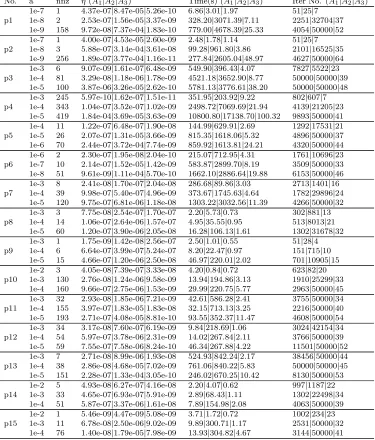
Table 1:The comparison results obtained by testing real data from the UCI and the BioNUS data sets with (w1, w2) set as in (19). A1:
the ADMM withτ= 1.618; A2: the APG method implemented by
No. a nnz η(A1|A2|A3) Time(s) (A1|A2|A3) Iter No. (A1|A2|A3)
1e-7 1 4.37e-07|8.47e-05|5.26e-10 6.86|3.01|1.97 51|25|7 p1 1e-8 2 2.53e-07|1.56e-05|3.37e-09 328.20|3071.39|7.11 2251|32704|37
1e-9 158 9.72e-08|7.37e-04|1.83e-10 779.00|4678.39|25.33 4054|50000|52 1e-7 1 4.00e-07|4.53e-05|2.60e-09 2.48|1.78|1.14 51|25|7 p2 1e-8 3 5.88e-07|3.14e-04|3.61e-08 99.28|961.80|3.86 2101|16525|35
1e-9 256 1.89e-07|3.77e-04|1.16e-11 277.84|2605.04|48.97 4627|50000|64 1e-3 6 9.07e-09|1.61e-07|6.48e-09 549.90|396.43|4.07 7827|5522|23 p3 1e-4 81 3.29e-08|1.18e-06|1.78e-09 4521.18|3652.90|8.77 50000|50000|39
1e-5 100 3.87e-06|3.26e-05|2.62e-10 5781.13|3776.61|38.20 50000|50000|48 1e-3 245 5.97e-10|1.62e-07|1.51e-11 351.95|203.92|9.22 802|607|7 p4 1e-4 343 1.04e-07|3.52e-07|1.02e-09 2498.72|7069.69|21.94 4139|21205|23
1e-5 419 1.84e-04|3.69e-05|3.63e-09 10800.80|17138.70|100.32 9893|50000|41 1e-4 11 1.22e-07|6.48e-07|1.90e-08 144.99|629.91|2.69 1292|17531|21 p5 1e-5 26 2.07e-07|1.31e-05|3.66e-09 815.35|1618.06|5.32 4896|50000|37 1e-6 70 2.44e-07|3.72e-04|7.74e-09 859.92|1613.81|24.21 4320|50000|44 1e-6 2 2.30e-07|1.95e-08|2.04e-10 215.07|712.95|4.31 1761|10696|23 p6 1e-7 10 2.14e-07|1.52e-05|1.42e-09 583.87|2899.70|8.19 3509|50000|33 1e-8 51 9.61e-09|1.11e-04|5.70e-10 1662.10|2886.64|19.88 6153|50000|46 1e-3 8 2.41e-08|1.70e-07|2.04e-08 286.68|89.86|3.03 2713|1401|16 p7 1e-4 39 9.98e-07|5.40e-07|4.96e-09 373.67|1745.63|4.64 1782|29896|24
1e-5 120 9.75e-07|6.81e-06|1.18e-08 1303.22|3032.56|11.39 4266|50000|32 1e-3 3 7.75e-08|2.54e-07|1.70e-07 2.20|5.73|0.73 302|881|13 p8 1e-4 14 1.06e-07|2.64e-06|1.57e-07 4.95|35.55|0.95 513|8013|21
1e-5 60 1.20e-07|3.90e-06|2.05e-08 16.28|106.13|1.61 1302|31678|32 1e-3 1 1.75e-09|1.42e-08|2.56e-07 2.50|1.01|0.55 51|28|4 p9 1e-4 6 6.64e-07|3.99e-07|5.24e-07 8.20|22.47|0.97 151|715|10
1e-5 15 4.66e-07|1.20e-06|2.50e-08 46.97|220.01|2.02 701|10905|15 1e-2 3 4.05e-08|7.39e-07|3.33e-08 4.20|0.84|0.72 623|82|20 p10 1e-3 130 2.76e-08|1.24e-06|9.58e-09 13.94|194.86|3.13 1910|25299|33
1e-4 160 9.66e-07|2.75e-06|1.53e-09 29.99|220.75|5.77 2963|50000|45 1e-3 32 2.93e-08|1.85e-06|7.21e-09 42.61|586.28|2.41 3755|50000|34 p11 1e-4 155 3.97e-07|1.83e-05|1.83e-08 32.15|713.13|3.25 2216|50000|40 1e-5 193 2.71e-07|4.08e-05|8.81e-10 93.55|352.37|11.47 4608|50000|54 1e-3 34 3.17e-08|7.60e-07|6.19e-09 9.84|218.69|1.06 3024|42154|34 p12 1e-4 54 5.97e-07|3.78e-06|2.31e-09 14.02|267.84|2.11 3766|50000|39 1e-5 59 7.55e-07|7.58e-06|8.24e-10 46.34|267.88|4.22 11501|50000|52 1e-3 7 2.71e-08|8.99e-06|1.93e-08 524.93|842.24|2.17 38456|50000|44 p13 1e-4 38 2.86e-08|4.68e-05|7.02e-09 761.06|840.22|5.83 50000|50000|45 1e-5 151 2.28e-07|1.33e-04|3.05e-10 246.02|670.25|10.42 8130|50000|53 1e-2 5 4.93e-08|6.27e-07|4.16e-08 2.20|4.07|0.62 997|1187|22 p14 1e-3 33 4.65e-07|6.93e-07|5.91e-09 2.89|68.43|1.11 1302|22498|34
1e-4 51 5.87e-07|3.37e-06|1.61e-08 7.89|154.98|2.08 4063|50000|39 1e-2 1 5.46e-09|4.47e-09|5.08e-09 3.71|1.72|0.72 1002|234|23 p15 1e-3 11 6.78e-08|2.50e-06|9.02e-09 9.89|300.71|1.17 2531|50000|32
1e-4 76 1.40e-08|1.79e-05|7.98e-09 13.93|304.82|4.67 3144|50000|41
p11 lung H1 [203, 12600] p12 NervousSystem [60, 7129] p13 ovarian P [253, 15153]
p14 DLBCL S [47, 4026]
p15 lung M [96, 7129]
From Table 1, we observe that all the 45 tested instances are successfully solved by Newt-ALM within 2 minutes (for most of the cases within less than half a minute), while 3 and 22 cases have failed (i.e., not achieving our stopping criteria) to be solved by ADMM and SLOPE, respectively. This shows that our Hessian based Newt-ALM algorithm is more robust compared to the first-order methods (ADMM and the accelerated proximal gradient method implemented in SLOPE) in its ability to successfully solve difficult problems. Both the solution accuracy (as shown in the column under “η”) and the computation time (as shown in the column under “Time(s)”) also show a tremendous computational advantage of Newt-ALM comparing to ADMM and SLOPE. In particular, for many of the instances corresponding to p3, p4, p5, p6, p7, p13, our algorithm can be more than 100 times faster than ADMM and SLOPE.
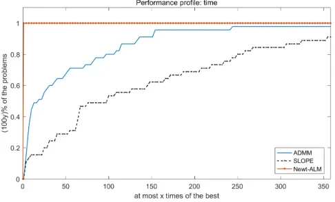
It is noteworthy that the dual-based ADMM also works better than SLOPE for majority of the tested instances. The performance profiles of these three algorithms for all 45 tested problems are presented in Figure 1. Recall that a point (x, y) on a particular profile curve implies that the algorithm can solve (100y)% of all the tested instances up to the desired accuracy within at mostxtimes of the fastest algorithm for each instance. More specifically, for x = 150, we can see from Figure 1 that even by consuming more than 150 times of the computation time taken by Newt-ALM, there are still around 40% and 10% of tested instances which are not successfully solved by SLOPE and ADMM, respectively.
Figure 1: Time comparison for ADMM, SLOPE and Newt-ALM.
4.4. Results on real data sets with group structures
The first one is the breast cancer data set compiled by Van de Vijver et al. (2002), which consists of gene expression data for 8,141 genes in 295 breast cancer tumors (78 metastatic and 217 non-metastatic). We restrict the analysis to 3510 genes which are in at least one pathway. Since the data set is very unbalanced, we adopt the balancing scheme in Jacob et al. (2009) by using 3 replicates of each metastasis tumor and yield a total number of 451 samples. The comparison results are listed in Table 3.
Table 3: The comparison results obtained by testing the breast can-cer data set with (w1, w2) set as in (19) with different values fora.
A1: ADMM with τ= 1.618; A2: the APG method in the SLOPE
package; A3: our Newt-ALM.
a nnz η(A1|A2|A3) Time(s) (A1|A2|A3) Iter No. (A1|A2|A3)
1e-3 145 1.43e-08|7.09e-07|2.48e-09 2.42|26.02|0.86 402|6220|20 1e-4 306 3.66e-08|8.74e-07|9.35e-10 10.21|70.51|2.80 1310|18016|33 1e-5 335 1.86e-09|7.12e-06|8.31e-10 34.63|205.39|4.68 3051|50000|43
The second data set is the NCEP/NCAR reanalysis 1 data set from Kalnay et al. (1996) which contains the monthly means of climate data measurements spread across the globe in a grid of 2.5o ×2.5o resolutions (longitude and latitude 144×73) from 1948/01/01 to 2018/05/31. Each grid point has 7 predictive variables including the air temperature, precipitable water, relative humidity, pressure, sea level pressure, horizontal wind speed and vertical wind speed, which leads to a natural group structure in the data set (each group of length 7). The resulting measurement matrix Ais of size [m, n] = 845×73584. Similar to the parameter scheme chosen in Ndiaye et al. (2016) and Zhang et al. (2018), we manually choose the tuning parameters w1 and w2 as follows:
w1= 0.4w(t) and w2 = 0.6w(t) (20)
with w(t) = 10−5+[3(t−1)/99]× kA>bk∞. The numerical results with different t’s are listed
in Table 4.
Table 4: The comparison results obtained by testing the NCEP/NCAR reanalysis 1 data set with (w1, w2) set as in (20).
A1: ADMM with τ= 1.618; A2: the APG method in the SLOPE
package; A3: our Newt-ALM.
t η(A1|A2|A3) Time(s) (A1|A2|A3) Iter No. (A1|A2|A3)
From Tables 3 and 4, we can draw a similar conclusion as the experiments on the UCI and the BioNUS data sets discussed in Subsection 4.3. That is, our Newt-ALM method is far superior to the tested first-order methods in terms of computational efficiency and the ability to successfully solve the problems to the required level of accuracy. 4.5. The pathwise solution for a microarray data
The behavior of the OSCAR model for sparse feature selection and grouping for each specific instance relies heavily on the tuning parametersw1 and w2. To get a reliable and effective
estimation for the coefficients of all involved predictors in the context of linear regression, a two-dimensional grid of various w1 and w2 values are tested to generate a solution path. The task of generating a solution path can be costly since each single pair of parameters (w1, w2) will lead to a different instance of the OSCAR model. The path usually begins with
appropriately chosen parameters that shrink all the coefficients to zero, and moves on until we are near the un-regularized solution by varying the values of the parameters. During the construction of the solution path, the warm start strategy (Friedman et al., 2007, 2010) is always used to accelerate the entire process by using the previous near-by solution as the initial point for the next problem.
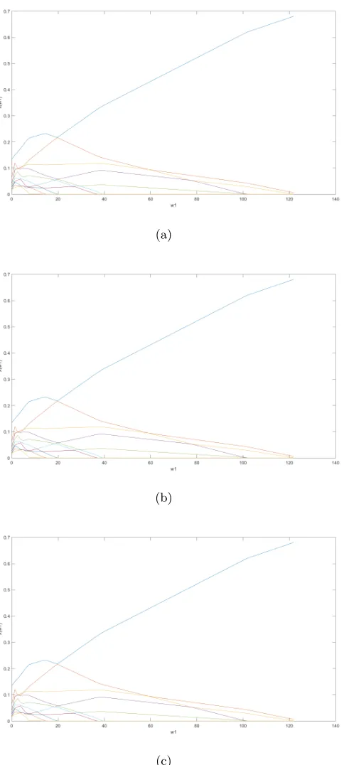
Here, we will use the microarray data set reported in Scheetz et al. (2006) and processed it by following Huang et al. (2008); Gu et al. (2018), where the design matrix A ∈ Rm×n
and the response vector b ∈ Rm with m = 120 and n = 3000. A partial solution path
with the parameterw2 fixed at the valuekA>bk∞/n2, and the parameterw1 varying evenly
in the interval 10−4,10−2× kA>bk∞ for 100 different values will be constructed. The
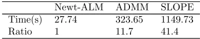
first 10 largest coefficients in magnitude of all the 100 numerical solutions are collected in Figure 2 by using ADMM, SLOPE and Newt-ALM, respectively. The timing comparison for generating the partial solution paths by these three algorithms is presented in Table 5.
Table 5: Computation time comparison among Newt-ALM,
ADMM and SLOPE for generating the partial solution paths, where the row “Ratio” reports the ratios of the computation time of each single algorithm to that of the fastest algorithm.
Newt-ALM ADMM SLOPE
Time(s) 27.74 323.65 1149.73
Ratio 1 11.7 41.4
(a)
(b)
(c)
high-dimensional linear regression, both the advantage in computation time and solution accuracy of our Newt-ALM will certainly be more significant, as can be observed in Table 1 and deduced from the computational complexity analysis in Subsection 3.4.
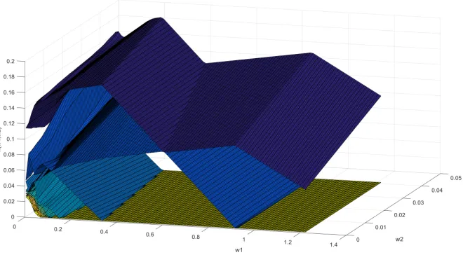
With a two-dimensional grid of varying w1 and w2 values, we can also construct a three-dimensional scattergram to show those first k (e.g., k = 10) largest components in magnitude for the microarray data. Figure 3 shows such a case, from which we can get a partial solution path along w1 (or w2) with any fixed w2 (or w1), or along any set of (w1, w2) pairs on the grid. Figure 3 shows the scattergram which collects the first 10 largest components in magnitude with w1 and w2 varying evenly in
10−7,10−4
× kA>bk∞ and
10−4,10−2×kA>bk∞/n, respectively. All the 10,000 problems are solved by our algorithm
Newt-ALM in a total of about 70 minutes.
Figure 3: The first 10 largest components in magnitude of solutions with a two-dimensional grid ofw1 and w2 values for the microarray data
5. Discussions
second-order differential information of the underlying structured regularizer. Besides the least squares loss function adopted in the OSCAR and SLOPE models, our method is also applicable for the case of the logistic loss function, in which the desired nice properties of the corresponding subproblems are maintained to guarantee the efficiency and robustness of the algorithm. For classical statistical regression with larger sample size, our method is still applicable. But we may have to explore whether it is more efficient to apply our algorithmic framework directly to the OSCAR and SLOPE models, instead of our current application to the dual problem. The efficiency and effectiveness of our algorithm in solving high-dimensional linear regression with the OSCAR and SLOPE regularizers will greatly facilitate data analysis in statistical learning and related applications across a broad range of fields.
Acknowledgments
Appendix A.
In this appendix we prove the following theorem from Section 2:
TheoremLet λ∈Rn
+ be such that λ1≥ · · · ≥λn. Then M(·) is a nonempty and compact
valued, upper semicontinuous multifunction, and for any given y ∈ Rn, every M ∈ M(y) is symmetric and positive semidefinite. Moreover, there exists a neighborhood U of y such that for all y0∈U,
Proxκλ(y
0)−Prox
κλ(y)−M(y
0−y) = 0, ∀M ∈ M(y0). (21)
Proof. Lety∈Rnbe an arbitrary point. Then it is obvious thatM(y) is a nonempty and
compact set. The symmetric and positive semidefiniteness of M ∈ M(y) is trivial by the definitions in (6) and (8). Now we claim that there exists a neighborhoodV ofy∈Rn such
that
Πs(y0)⊆Πs(y), ∀y0∈V.
This claim is trivial for y = 0 since Πs(0) = Πsn. For the case of a nonzero y ∈ Rn, let r
be the number of distinct values in|y|, and t1,. . .,tr be all those distinct values satisfying
t1 > t2>· · ·> tr ≥0. Consider the following two cases:
Case I: Iftr >0, set δ:= 13min
tr, min
1≤i≤r−1{ti−ti+1}
;
Case II: If tr= 0, setδ := 13 min
1≤i≤r−1{ti−ti+1}.
It is easy to verify that in both casesδ >0 and
Πs(y0)⊆Πs(y), ∀y0∈B(y, δ), (22)
where B(y, δ) is the 2-norm ball centered at y with radius δ. The upper semicontinuity of
M then can be obtained from (22) and (7). The remaining part is to show (21). For any
y0∈B(y, δ) withδ defined as above, it is known from (5) and the inclusion property in (22) that
Proxκλ(y
0)−Prox
κλ(y) =π −1 x
λ(πy0)−xλ(πy)
, ∀π ∈Πs(y0). (23) By combining the properties in (7) and the fact thatkπy0−πyk=ky0−yk, we know that there exists a neighborhoodU ⊆B(y, δ) ofy such that for ally0 ∈U,
xλ(πy0)−xλ(πy) =P(πy0−πy), ∀P ∈P(πy0),∀π∈Πs(y0),
which together with (23) leads to the desired result in (21). This completes the proof.
References
Jean-Pierre Aubin and H´el`ene Frankowska. Set-Valued Analysis. Birkh¨auser, 1990.
Richard E. Barlow and H. D. Brunk. The isotonic regression problem and its dual. Journal of the American Statistical Association, 67(337):140–147, 1972.
Ma lgorzata Bogdan, Ewout van den Berg, Chiara Sabatti, Weijie Su, and Emmanuel J. Cand`es. SLOPE-adaptive variable selection via convex optimization. The Annals of Applied Statistics, 9(3):1103–1140, 2015.
Howard D. Bondell and Brian J. Reich. Simultaneous regression shrinkage, variable selec-tion, and supervised clustering of predictors with OSCAR. Biometrics, 64(1):115–123, 2008.
Liang Chen, Defeng Sun, and Kim-Chuan Toh. An efficient inexact symmetric Gauss-Seidel based majorized ADMM for high-dimensional convex composite conic program-ming. Mathematical Programming, Series A, 161(1-2):237–270, 2017.
Scott Shaobing Chen, David L. Donoho, and Michael A. Saunders. Atomic decomposition by basis pursuit. SIAM Journal on Scientific Computing, 20:33–61, 1998.
Ying Cui, Defeng Sun, and Kim-Chuan Toh. On the R-superlinear convergence of the KKT residuals generated by the augmented lagrangian method for convex composite conic programming. Mathematical Programming, DOI: 10.1007/s10107-018-1300-6, 2018.
Maryam Fazel, Ting Kei Pong, Defeng Sun, and Paul Tseng. Hankel matrix rank minimiza-tion with applicaminimiza-tions to system identificaminimiza-tion and realizaminimiza-tion. SIAM Journal on Matrix Analysis and Applications, 34(3):946–977, 2013.
Mario A. T. Figueiredo, Robert D. Nowak, and Stephen J. Wright. Gradient projection for sparse reconstruction: Application to compressed sensing and other inverse problems.
IEEE Jounral of Selected Topics in Signal Processing, 1:586–597, 2007.
Jerome Friedman, Trevor Hastie, Holger H¨ofling, and Robert Tibshirani. Pathwise coordi-nate optimization. The Annals of Applied Statistics, 1(2):302–332, 2007.
Jerome Friedman, Trevor Hastie, and Robert Tibshirani. Regularization paths for gener-alized linear models via coordinate descent. Journal of Statistical Software, 33(1):1–22, 2010.
Daniel Gabay and Bertrand Mercier. A dual algorithm for the solution of nonlinear vari-ational problems via finite element approximation. Computers and Mathematics with Applications, 2(1):17–40, 1976.
Roland Glowinski and Americo Marrocco. Sur l’approximation, par ´el´ements finis d’ordre un, et la r´esolution, par p´enalisation-dualit´e d’une classe de probl`emes de dirichlet non lin´eaires. Revue fran¸caise d’atomatique, Informatique Recherche Op´erationelle. Analyse Num´erique, 9(2):41–76, 1975.
Yuwen Gu, Jun Fan, Lingchen Kong, Shiqian Ma, and Hui Zou. ADMM for high-dimensional sparse penalized quantile regression. Technometrics, 60(3):319–331, 2018.
Ronald R. Hocking. The analysis and selection of variables in linear regression. Biometrics, 32:1–49, 1976.
Jian Huang, Shuangge Ma, and Cun-Hui Zhang. Adaptive lasso for sparse high-dimensional regression models. Statistica Sinica, 18(4):1603–1618, 2008.
Laurent Jacob, Guillaume Obozinski, and Jean Philippe Vert. Group lasso with overlap and graph lasso. InInternational Conference on Machine Learning, pages 433–440, 2009.
E. Kalnay, M. Kanamitsu, R. Kistler, W. Collins, D. Deaven, L. Gandin, M. Iredell, S. Saha, G. White, J. Woollen, Y. Zhu, M. Chelliah, W. Ebisuzaki, W. Higgins, J. Janowiak, K. C. Mo, C. Ropelewski, J. Wang, A. Leetmaa, R. Reynolds, R. Jenne, and Joseph J. D. The NCEP/NCAR 40-year reanalysis project.Bulletin of the American Meteorological Society, 77:437–472, 1996.
Bernd Kummer. Newton’s method for non-differentiable functions. Advances in Mathemat-ical Optimization, 45:114–125, 1988.
Xudong Li, Defeng Sun, and Kim-Chuan Toh. An efficient linearly convergent semismooth Netwon-CG augmented lagrangian method for Lasso problems. SIAM Journal on Opti-mization, 28(1):433–458, 2018a.
Xudong Li, Defeng Sun, and Kim-Chuan Toh. On efficiently solving the subproblems of a level-set method for fused lasso problems. SIAM Journal on Optimization, 28:1842–1866, 2018b.
Moshe Lichman. UCI machine learning repository. http://archive.ics.uci.edu/ml/ datasets.html, 2013.
Julien Mairal, Francis Bach, and Jean Ponce. Sparse modeling for image and vision pro-cessing. Foundations and Trends in Computer Graphics and Vision, 8:85–283, 2014.
Robert Mifflin. Semismooth and semiconvex functions in constrained optimization. SIAM Journal on Control and Optimization, 15(6):959–972, 1977.
Alan Miller. Subset Selection in Regression. Chapman & Hall, London, UK, 2002.
Jean-Jacques Moreau. Proximit´e et dualit´e dans un espace hilbertien. Bulletin de la Socie´te´
Mathe´matique de France, 93(2):273–299, 1965.
Eugene Ndiaye, Olivier Fercoq, Alexandre Gramfort, and Joseph Salmon. GAP safe screen-ing rules for sparse-group lasso. In Advances in Neural Information Processing Systems 29 (NIPS 2016), pages 388–396, 2016.
Yurii Nesterov. A method of solving a convex programming problem with convergence rate
o(1/k2). Soviet Mathematics Doklady, 27(2):372–376, 1983.
Franck Rapaport, Andrei Zinovyev, Marie Dutreix, Emmanuel Barillot, and Jean-Philippe Vert. Classification of microarray data using gene networks. BMC Bioinformatics, 8:35, 2007.
Tim Robertson, Farroll T. Wright, and Richard Dykstra. Order Restricted Statistical In-ference. Wiley Series in Probability and Mathematical Statistics: Probability and Math-ematical Statistics. John Wiley & Sons, Chichester, 1988. ISBN 0-471-91787-7.
Stephen M. Robinson. Some continuity properties of polyhedral multifunctions. Mathemat-ical Programming Study, 16:206–214, 1981.
Ralph Tyrell Rockafellar. Convex Analysis. Princeton University Press, 1970.
Ralph Tyrell Rockafellar. Monotone operators and the proximal point algorithm. SIAM Journal on Control and Optimization, 14(5):877–898, 1976a.
Ralph Tyrell Rockafellar. Augmented Lagrangians and applications of the proximal point algorithm in convex programming. Mathematics of Operations Research, 1(2):97–116, 1976b.
Ralph Tyrell Rockafellar and Roger J-B Wets.Variational Analysis. Springer-Verlag, Berlin, 1998.
Todd E. Scheetz, Kwang-Youn A. Kim, Ruth E. Swiderski, Alisdair R. Philp, Terry A. Braun, Kevin L. Knudtson, Anne M. Dorrance, Gerald F. DiBona, Jian Huang, and Thomas L. Casavant. Regulation of gene expression in the mammalian eye and its rel-evance to eye disease. Proceedings of the National Academy of Sciences, 103(39):14429– 14434, 2006.
Mervyn J. Silvapulle and Pranab Kumar Sen. Constrained Statistical Inference: Order, Inequality, and Shape Constraints, volume 912. John Wiley & Sons, 2011.
Defeng Sun and Jie Sun. Semismooth matrix-valued functions. Mathematics of Operations Research, 27(1):150–169, 2002.
Jie Sun. On monotropic piecewise quadratic programming. PhD thesis, University of Wash-ington, 1986.
Robert Tibshirani. Regression shrinkage and selection via the LASSO. Journal of the Royal Statistical Society, 58:267–288, 1996.
Joel A. Tropp. Just relax: Convex programming methods for identifying sparse signals.
IEEE Transactions on Information Theory, 51:1030–1051, 2006.
Yuhang Wang, Fillia S. Makedon, James C. Ford, and Justin Pearlman. Hykgene: a hybrid approach for selecting marker genes for phenotype classification using microarray gene expression data. Bioinformatics, 21:1530–1537, 2005.
Bin Wu, Chao Ding, Defeng Sun, and Kim-Chuan Toh. On the Moreau–Yosida regular-ization of the vector k-norm related functions. SIAM Journal on Optimization, 24(2): 766–794, 2014.
Xiangrong Zeng and M´ario AT Figueiredo. Solving OSCAR regularization problems by proximal splitting algorithms. Digital Signal Processing, 31:124–135, 2014a.
Xiangrong Zeng and M´ario AT Figueiredo. Decreasing weighted sorted `1 regularization.
IEEE Signal Processing Letters, 21(10):1240–1244, 2014b.
Yangjing Zhang, Ning Zhang, Defeng Sun, and Kim-Chuan Toh. An efficient hessian based algorithm for solving large-scale sparse group lasso problems.Mathematical Programming, DOI:10.1007/s10107-018-1329-6, 2018.