High-Dimensional Poisson Structural Equation Model
Learning via
`
1-Regularized Regression
Gunwoong Park [email protected]
Department of Statistics University of Seoul Seoul, 02504, South Korea
Sion Park [email protected]
Department of Statistics University of Seoul Seoul, 02504, South Korea
Editor:Qiang Liu
Abstract
In this paper, we develop a new approach to learning high-dimensional Poisson structural equation models from only observational data without strong assumptions such as faithful-ness and a sparse moralized graph. A key component of our method is to decouple the or-dering estimation or parent search where the problems can be efficiently addressed using`1
-regularized regression and the moments relation. We show that sample sizen= Ω(d2log9p)
is sufficient for our polynomial time Moments Ratio Scoring (MRS) algorithm to recover the true directed graph, wherepis the number of nodes and dis the maximum indegree. We verify through simulations that our algorithm is statistically consistent in the high-dimensionalp > nsetting, and performs well compared to state-of-the-art ODS, GES, and MMHC algorithms. We also demonstrate through multivariate real count data that our MRS algorithm is well-suited to estimating DAG models for multivariate count data in comparison to other methods used for discrete data.
Keywords: Bayesian Networks, Directed Acyclic Graph, Identifiability, Structure Learn-ing,`1-Regularization, Multivariate Count Distribution
1. Introduction
Directed acyclic graphical (DAG) models, also referred to as Bayesian networks, are popular probabilistic statistical models to analyze and visualize (functional) causal or directional dependence relationships among random variables.(see e.g., Kephart and White, 1991; Fried-man et al., 2000; Doya, 2007; Peters and B¨uhlmann, 2014). However, learning DAG models from only observational data is a notoriously difficult problem due to non-identifiability and exponentially growing computational complexity. Prior works have addressed the question of identifiability for different classes of joint distributionP(G). Frydenberg (1990) and Heck-erman et al. (1995) show the Markov equivalence class (MEC) where graphs that belong to the same MEC have the same conditional independence relations. Spirtes et al. (2000), Chickering (2003), Tsamardinos and Aliferis (2003) and Zhang and Spirtes (2016) show that the underlying graph of a DAG model is recoverable up to the MEC under faithfulness or related assumptions that can be very restrictive (Uhler et al., 2013).
c
Also well studied is how learning a DAG model is computationally non-trivial due to the super-exponentially growing size of the space of DAGs in the number of nodes. Hence, it is NP-hard to search DAG space (Chickering et al., 1994; Chickering, 1996), and many existing algorithms such as PC (Spirtes et al., 2000), Greedy Equivalence Search (GES) (Chickering, 2003), Min-Max Hill Climbing (MMHC) (Tsamardinos et al., 2006) and Greedy DAG Search (GDS) (Peters and B¨uhlmann, 2014), take greedy search methods that may not guarantee to recover the true MEC.
Recently, a number of fully identifiable classes of DAG models have been introduced (Shimizu et al., 2006; Hoyer et al., 2009; Peters et al., 2011; Peters and B¨uhlmann, 2014; Park and Raskutti, 2015, 2018; Ghoshal and Honorio, 2018; Park and Park, 2019). In addition, some of these models can be successfully learned from high-dimensional data by decomposing the DAG learning problem into ordering estimation and skeleton estima-tion (Shimizu et al., 2011; B¨uhlmann et al., 2014; Ghoshal and Honorio, 2017b; Drton et al., 2018). The main reasoning is that if ordering is known or recoverable, learning a directed graphical model is as hard as learning an undirected graphical model or Markov random field (MRF). Meinshausen and B¨uhlmann (2006), Wainwright et al. (2006), Ravikumar et al. (2011) and Yang et al. (2015) show that sparse undirected graphs can be estimated via `1-regularized regression in high-dimensional settings under suitable conditions.
In this paper, we focus on learning Poisson DAG models (Park and Raskutti, 2015, 2018) for multivariate count data in high-dimensional settings since large-scale multivariate
count data frequently arises in many fields, such as high-throughput genomic sequencing data, spatial incidence data, sports science data, and disease incidence data. Like learning the Poisson undirected graphical model or MRF introduced in Yang et al. (2015), where the sample bound is Ω(d2
mlog3p), it is not surprising that Poisson DAG models can be
learned in high dimensional settings when the indegree of the graph d is bounded. Park and Raskutti (2018) establishes the consistency of learning Poisson DAG models with the sample bound n = Ω(max{d4
mlog12p,log5+dp}) where dm is the maximum degree of the
moralized graph anddis the maximum indegree of a graph. This huge sample complexity difference between directed and undirected graphical models is induced mainly for three reasons: (i) nonexistence ordering, (ii) the known parametric functional form (the standard log link) for the dependencies, and (iii) the restrictive non-positive parameter space in Poisson MRFs (see details in Yang et al., 2015).
close to the information-theoretic limit of Ω(dlogp) for learning sparse DAG models with any exponential family distributions (Ghoshal and Honorio, 2017a). We point out that the sample complexity does not depend on the maximum degree of the moralized graph, dm,
but on the indegree of a DAG,d. Since a sparse directed graph does not necessarily lead to the sparse moralized graph (e.g., a star graph in Fig. 2), to the best of our knowledge, the proposed algorithm is the most efficient and probable for learning sparse Poisson SEMs.
We demonstrate through simulations and a real baseball data application involving mul-tivariate count data that our MRS algorithm performs better than state-of-the-art OverDis-persion Scoring (ODS) (Park and Raskutti, 2015), GES (Chickering, 2003), MMHC (Tsamardi-nos et al., 2006), and Poisson MRF learning (PMRF) algorithms (Yang et al., 2015), on average, in terms of the both run-time and accuracy of recovering a graph structure and its MEC. In our simulation study, we consider both the extremely sparse (d= 1) and sparse (d= 10) high-dimensional settings. Our real data example involving MLB player statistics for 2003 season shows that our MRS algorithm is applicable to multivariate count data while the PMRF algorithm finds too many edges, and the MMHC algorithm tends to select very few edges when variables represent counts. We also investigate the accuracy of our MRS algorithm when samples are generated from general Poisson DAG models and (trun-cated) Poisson MRFs. The simulation results empirically verify that the MRS algorithm can consistently recover the true edges.
1.1. Our Contributions
We summarize the major contributions of the paper as follows:
• We introduce a milder identifiability condition for Poisson DAG models for multivari-ate count data.
• We develop the reliable and scalable lasso-based MRS algorithm which learns sparse high-dimensional Poisson SEMs.
• We provide the more realistic conditions for learning Poisson SEMs in Section 3.2.
• We also provide the sample complexityn= Ω(d2log9p) under which the MRS algo-rithm recovers the Poisson SEM. We emphasize that our theoretical result does not depend on the degree of the moralized graphdm, and hence, the MRS algorithm can
recover a graph with hub nodes in the high dimensional setting.
To the best of our knowledge, our MRS algorithm is the only provable and realistic method that applies for the high-dimensional multivariate count data when samples are from Poisson SEMs with hub nodes. We must point out that such improved assumptions and sample complexity are not only from our new identifiability condition, but from the additional constraints on the standard log link function for the dependencies.
computational complexity of our algorithm, and Section 3.2 provides statistical guarantees for learning Poisson SEMs via the MRS algorithm. Section 4 empirically evaluates our methods, compared to state-of-the-art ODS, GES, and MMHC algorithms using synthetic data, and confirms that our algorithm is one of the few DAG-learning algorithms that per-forms well in terms of statistical and computational complexity in low and high-dimensional settings. In addition, we investigate how well the MRS algorithm learns general Poisson DAG models and (truncated) Poisson MRFs using synthetic data. Section 5 compares our MRS algorithm to the Poisson MRF and MMHC algorithm by analyzing a real 2003 season MLB multivariate count data. Lastly, Section 6 discusses some future works.
2. Poisson DAG Models
We first introduce some necessary notations and definitions for DAG models. Then, we give a detailed description of previous work on learning Poisson DAG models (Park and Raskutti, 2015), and we propose a strictly milder identifiability condition. Lastly, we discuss how Poisson DAG models and MRFs (Yang et al., 2015) are related.
2.1. Problem Set-up and Notations
A DAGG= (V, E) consists of a set of nodes V ={1,2,· · ·, p} and a set of directed edges
E ⊂V ×V with no directed cycles. A directed edge from nodej tok is denoted by (j, k) orj→k. The set ofparents of nodek, denoted by Pa(k), consists of all nodesj such that (j, k) ∈ E. If there is a directed path j → · · · → k, then k is called a descendant of j, and j is anancestor of k. The set De(k) denotes the set of all descendants of node k. The
non-descendants of nodekare Nd(k) :=V\({k} ∪De(k)). An important property of DAGs is that there exists a (possibly non-unique) ordering π = (π1, ...., πp) of a directed graph
that represents directions of edges such that for every directed edge (j, k) ∈ E, j comes beforekin the ordering. Hence, learning a graph is equivalent to learning the ordering and the skeleton that is the set of directed edges without their directions.
We consider a set of random variables X := (Xj)j∈V with a probability distribution
taking values in a sample spaceXV over the nodes inG. Suppose that a random vectorX
has a joint probability density function P(G) =P(X1, X2, ..., Xp). For any subset S of V,
let XS := {Xj : j ∈ S ⊂ V} and XS := ×j∈SXj where Xj is a sample space of Xj. For
any node j ∈V, P(Xj |XS) denotes the conditional distribution of a variable Xj given a
random vectorXS. Then, a DAG model has the following factorization (Lauritzen, 1996):
P(G) =P(X1, X2, ..., Xp) = p
Y
j=1
P(Xj |XPa(j)), (1)
where P(Xj | XPa(j)) is the conditional distribution of Xj given its parents variables XPa(j):={Xk:k∈Pa(j)⊂V}.
We suppose that there are n independent and identically distributed samples X1:n := (X(i))n
i=1 from a given graphical model where X(i) := X (i) 1:p = (X
(i) 1 , X
(i)
2 ,· · ·, X (i)
p ) is ap
-variate random vector. The notationb·denotes an estimate based on samplesX
1:n. We also
2.2. Poisson DAG Model and its Identifiability
The definition of Poisson DAG models in Park and Raskutti (2015) is that each conditional distribution given its parents Xj |XPa(j) is Poisson such that
Xj |XPa(j) ∼Poisson(gj(XPa(j))), (2)
where for any arbitrary positive link functiongj :XPa(j)→R+. Hence using the factoriza-tion in Equafactoriza-tion (1), the joint distribufactoriza-tion is as follows:
fG(X) =
Y
j∈V
fj(Xj |XPa(j)). (3)
wherefj is the probability density function of Poisson.
A Poisson structural equation model (SEM) is a special case of a Poisson DAG model where the link functions gj’s in Equation (2) are the standard log link function for
Pois-son generalized linear models (GLMs), i.e., gj(XPa(j)) = exp(θj+Pk∈Pa(j)θjkXk) where
(θjk)k∈Pa(j) represents the linear weights. Using factorization (1), the joint distribution of
a Poisson SEM can be written as:
f(X1, X2, ..., Xp) = exp
X
j∈V
θjXj +
X
(k,j)∈E
θjkXjXk−
X
j∈V
logXj!−
X
j∈V eθj+
P
k∈Pa(j)θjkXk
.
(4)
Poisson DAG models have a useful moments relation for the identifiability:
Proposition 1 Consider a Poisson DAG model (3) with non-degenerated rate parameter functions(gj(XPa(j)))j∈V. Then, for any nodej∈V, and any setSj ⊂Nd(j), the following moments relation holds:
E(Xj2)
EE(Xj |XSj) +E(Xj |XSj)2
≥1 (5)
Equivalently,
E(Var(E(Xj |XPa(j))|XSj))≥0.
The equality only holds whenSj contains all parents of j, that is, Pa(j)⊂Sj.
We include the proof in Section A. Proposition 1 claims that when all parents of j, Pa(j), contribute to its rate parameter, the moments ratio in Equation (5) is equal to 1 if a condition set Sj contains all parents of j, Pa(j) ⊂ Sj, otherwise greater than 1. In
Poisson SEMs, it is clear that the non-degenerated rate parameter function assumptions are equivalent to the non-zero coefficients conditions, |θjk| > 0 for all k ∈ Pa(j) since gj(XPa(j)) = exp(θj+Pk∈Pa(j)θjkXk).
Now, we briefly explain how Poisson DAG models are identifiable from the moments ratio in Proposition 1 using the bivariate Poisson DAG models illustrated in Fig. 1: G1 :X1 ∼ Poisson(λ1), X2 ∼Poisson(λ2), whereX1 and X2 are independent;G2 :X1 ∼Poisson(λ1)
X1 X2
G1
X1 X2
G2
X1 X2
G3
Figure 1: Bivariate directed acyclic graphs ofG1,G2, and G3.
By Proposition 1, we can see thatE(Xj2) =E(Xj) +E(Xj)2 for all j∈ {1,2} inG1. In G2, we can also see that
E(X12) =E(X1) +E(X1)2, and E(X22)>E(X2) +E(X2)2.
Similarly, inG3, we haveE(X12)>E(X1) +E(X1)2, whileE(X22) =E(X2) +E(X2)2. Hence,
we can determine the true graph based on the moments ratio E(Xj2)/(E(Xj) +E(Xj)2).
This idea of a moments relation in Proposition 1 can easily apply to general p-variate Poisson DAG models, and hence, the models are identifiable by testing whether the moments ratio in Equation (5) is equal to 1 or greater than 1.
Theorem 2 Consider a Poisson DAG model (3) with rate parameters (gj(XPa(j)))j∈V. If for any j ∈ V, rate parameter gj(·) is non-degenerated, the Poisson DAG model is identifiable.
We include the proof in Section 3.2. Theorem 2 claims that any Poisson DAG model is identifiable if all parents of nodejcontribute to its rate parameter. Hence, Theorem 2 shows that any Poisson SEM is identifiable under the non-zero coefficients condition,|θjk|>0 for
all k ∈ Pa(j). This condition is also commonly assumed in (Gaussian) linear structural equation models for the model identifiability (Spirtes, 1995; Ghoshal and Honorio, 2017b, 2018; Loh and B¨uhlmann, 2014; Peters and B¨uhlmann, 2014; Park and Park, 2019). We believe that it is a natural condition that is in accordance with the intuitive understanding of relationships among variables.
Our identifiability condition is strictly milder than the previous identifiability result in Park and Raskutti (2015) that is equivalent to Var(E(Xj |XPa(j))|XSj =x)>0 for allx∈
XSj when Pa(j)6⊂Sj . For a better comparison, we consider a fully connected graph where X1∼Poisson(λ),X2 |X1 ∼Poisson(λ+X1), andX3 |X1, X2 ∼Poisson(λ+X21(X1 6= 0))
where λ is a positive constant and 1(·) is an indicator function. In this case, we can see Var(E(X3 | X1, X2) | X1 = 0) = 0, and hence, the identifiability condition in Park and Raskutti (2015) is not satisfied, while our condition is satisfied.
In a Poisson SEM, the identifiability assumption in Park and Raskutti (2015) is also satisfied under the non-zero coefficients condition. However, in the finite sample setting, the difference of both assumptions gets more crucial. For a positive constant c, Park and Raskutti (2015) requires minx∈XSj Var(E(Xj | XPa(j)) | XSj = x)) > c, while we need
E(Var(E(Xj |XPa(j))|XSj))> c. Hence, our new identifiability assumption makes
learn-ing Poisson SEMs easier. We discuss this more in Section 3.2.
2.3. Comparison to Poisson MRF
the comparison, we consider the joint distribution of a Poisson SEM in Equation (4). This is a form similar to the joint distribution of Poisson MRFs in Yang et al. (2015), where the joint distribution has the following form:
f(X1, X2, ..., Xp) = exp
X
j∈V
θjXj +
X
(k,j)∈E
θjkXjXk−
X
j∈V
logXj!−A(θ)
, (6)
whereA(θ) is the log of the normalization constant. The key difference between a Poisson SEM and a Poisson MRF is the normalization constant A(θ) in Equation (6), as opposed to the termP
j∈V e θj+P
k∈Pa(j)θjkXk in Equation (4), which depends on variables.
Yang et al. (2015) proves that a Poisson MRF (6) is normalizable if and only if all (θjk) values are less than or equal to 0. This means Poisson MRFs only capture negative
dependency relations. In addition, Yang et al. (2015) addresses the learning Poisson MRFs when the functional form of dependencies isXj |XV\j ∼Poisson(exp(θj+Pk∈N(j)θjkXk))
whereN(j) denotes the neighbors of a node j in the graph.
While Poisson MRFs have strong restrictions on the functional form for dependencies and the parameter space, they can be successfully learned in the high-dimensional settings with less restrictive constraints of sparsity. Yang et al. (2015) shows that Poisson MRFs can be recovered via `1-regularized regression if n= Ω d2mlog3p, where dm is the degree
of the undirected graph. In contrast, Park and Raskutti (2018) shows that Poisson DAG models can be learned via the ODS algorithm ifn= Ω(max{d4
mlog12p,log5+dp}) wheredm
is obtained by the moralized graph anddis the maximum indegree of the graph. This big difference in the sample complexity primarily comes from the unknown functional form for the dependencies in Poisson DAG models. In the next section, we will show that a significant advantage can be achieved by assuming the parametric function for the dependencies in terms of recovering the graphs.
3. Algorithm
Here, we present our Moments Ratio Scoring (MRS) algorithm for learning the identifiable Poisson SEM (4). Our algorithm alternates between an element-wise ordering search using the (conditional) moments ratio, and a parent search using `1-regularized GLM. Hence, the algorithm chooses a node for the first element of the ordering, and then determines its parents. The algorithm iterates this procedure until the last element of the ordering and its parents are determined.
Without loss of generality, assume that π = (1,2,· · ·, p) is the true ordering. Then Poisson SEMs (4) have the conditional distribution of Xj given that all variables before j
in the ordering are reduced to the following Poisson GLM:
P(Xj |X1:(j−1)) = exp
θjXj+
X
k∈1:(j−1)
θjkXkXj+ logXj!−exp
θj +
X
k∈1:(j−1) θjkXk
,
(7)
Our MRS (Algorithm 1) involves learning the ordering by comparing moments ratio scores of nodes using the following equations:
b
S(1, j) := Eb(X
2 j)
b
E(Xj) +Eb(Xj)2
and S(b m, j) :=
b
E(Xj2)
b
E Eb(Xj |X
b
π1:(m−1)) +Eb(Xj |Xπb1:(m−1))
2,
(8)
where π1:b m = {π1, ...,b bπm}, E(b Xj) =
1 n
Pn
i=1X (i)
j , and E(b E(b Xj | XS)) = 1n Pn
i=1exp θbjS+ P
k∈SbθjkSX
(i) k
, and Eb(Eb(Xj | XS)2) = 1
n
Pn
i=1exp 2θbjS+ 2 P
k∈SθbSjkX
(i) k
where bθS(j) =
(θbjS,θbS\j) is the solution of the following`1-regularized GLM:
b
θS(j) := arg min
1 n n X i=1
−Xj(i)
θj+
X
k∈S
θjkXk(i)
+ exp
θj+
X
k∈S
θjkXk(i)
+λj
X
k∈S
|θjk|.
(9)
This score is an estimator of the moments ratio relation in Equation (5). Hence, the correct element of the ordering has a score of 1, otherwise strictly greater than 1 in pop-ulation. The ordering is determined one node at a time by selecting the node with the smallest score. Similar strategies of element-wise ordering learning can be found in many existing algorithms (e.g., Shimizu et al., 2011; Ghoshal and Honorio, 2017b, 2018; Drton et al., 2018).
The novelty of our algorithm is learning an ordering by testing which nodes have the smallest moments ratio in Equation (5) using the `1-regularized GLM. By substituting the estimation of parametersθ(j) for an estimation of the conditional mean, we gain significant computational and statistical improvements compared to the previous works in Park and Raskutti (2015, 2018) where the method of moments is used for estimating the conditional mean and variance.
In principle, the number of conditional variances exponentially grows in the number of conditioning variables. Hence, if a conditioning set contains d-variables with 10 possible outcomes, then the number of possible computations is 10d. In other words, the minimum sample size for the ODS algorithm to be implemented is possibly 10d, otherwise, none of
conditional variances can be estimated.
As we discussed, the problem of a learning directed graph structure is the same as the problem of an learning undirected graph structure if the ordering is known. Hence, given the estimated ordering, the parents of each node j can be learned via`1-regularized GLM (see details in Meinshausen and B¨uhlmann, 2006; Wainwright et al., 2006; Ravikumar et al., 2011; Yang et al., 2015). Therefore, we determine the estimated parents of a node j as
c
Pa(j) :={k∈S:θbjkS 6= 0}where S=πb1:(j−1) and bθS(j) is the solution to Equation (9).
3.1. Computational Complexity
The computational complexity for the MRS algorithm involves the `1-regularized GLM
algorithm (Friedman et al., 2009) where the worse-case complexity is O(np) for a single
Algorithm 1: Moments Ratio Scoring (MRS)
Input : n i.i.d. samples,X1:n
Output: Estimated ordering bπ= (bπ1, ...,πbp) and an edge structure,Eb ⊂V ×V
Setπb0=∅;
for m={1,2,· · ·, p} do Set S={πb1,· · · ,bπm−1};
for j∈ {1,2,· · · , p} \S do
Estimate θbS(j) for `1-regularized generalized linear model (9);
Calculate scores S(bm, j) using Equation (8);
end
The mth element of the ordering,
b
πm = arg minjS(bm, j);
The parents of the mth element of the ordering,
c
Pa(bπm) ={k∈S|θbS
b
πmk6= 0};
end
Return: Estimate the edge set, Eb =∪m∈V{(k,πbm)|k∈Pa(c bπm)}
gradient in O(p) operations. Hence, with d non-zero terms in the GLM, a complete cycle costsO(pd) operations if no new variables become non-zero, and costs O(np) for each new variable entered (see details in Friedman et al., 2010). Since our algorithm hasp iterations and there arep−j+1 regressions withj−1 features for thejth iteration, the total worst-case complexity is O(np3).
The estimation of a Poisson MRF also involves a node-wise `1-regularized GLM over all other variables, and hence the worse-case complexity is O(np2) if the coordinate de-scent method is exploited. The addition of estimation of ordering makes p times more computationally inefficient than the standard method for learning Poisson MRFs.
Learning a DAG model is NP-hard in general (Chickering et al., 1994). Hence, many state-of-the-art MEC and DAG learning algorithms, such as PC (Spirtes et al., 2000), GES (Chickering, 2003), and MMHC (Tsamardinos et al., 2006), are inherently greedy search algorithms. In the numerical experiments in Section 4, we compare MRS to greedy hill-climbing search-based GES and MMHC algorithms in terms of run time, and show that MRS has a significantly better computational complexity.
3.2. Theoretical Guarantees
In this section, we provide theoretical guarantees on the MRS algorithm for learning Poisson SEMs (4). The main result is expressed in terms of the triple (n, p, d), wherenis a sample size, pis a graph node size, and dis the indegree of a graph.
3.2.1. Assumptions
We begin by discussing the assumptions we impose on Poisson SEMs. Since we apply
`1-regularized regression for the parent selection, most assumptions are similar to those
Important quantities are the Hessian matrices of the negative conditional log-likelihood of a nodej given some subsets of the nodes in the ordering, Sj ∈ {{π1},{π1, π2}, ...,{π1, ... , πj−1}}. LetQj,Sj :=52`jSj(θ∗S(j);X1:n) where
`Sjj(θSj(j), X
1:n) := 1 n
n
X
i=1
−Xj(i)
θjSj + X
k∈Sj
θjkSjXk(i)
+ exp
θSjj+ X
k∈Sj
θSjkjXk(i)
,
(10)
θ∗Sj(j) := arg minE
−Xj
θSjj+ X
k∈Sj θSjkjXk
+ exp
θSjj+ X
k∈Sj θSjkjXk
. (11)
For ease of notation, we define a set for the non-zero elements of θS∗ j(j),
Tj :={k∈Sj |θ∗jk 6= 0 where θ ∗
Sj(j) = (θ ∗ j, θ
∗
jk)}. (12)
We note that if Sj contains all parents of j, Pa(j) ⊂ Sj, then Tj = Pa(j). Lastly, for
simplicity, we let ASS denote the |S| × |S| sub-matrix of the matrix A corresponding to
variables XS.
Assumption 1 (Dependence Assumption) For anyj ∈V and anySj ∈ {{π1},{π1, π2}, ...,{π1, ..., πj−1}}, there exist positive constants ρmin and ρmax such that
min
j∈V λmin
Qj,Sj TjTj
≥ρmin, and max j∈V λmax
1
n n
X
i=1 XPa(i)
(j)(X (i) Pa(j))
T
!
≤ρmax,
where Tj is in Equation (12),λmin(A) andλmax(A) are the smallest and largest eigenvalues of the matrix A, respectively.
Assumption 2 (Incoherence Assumption) For anyj∈V and anySj ∈ {{π1},{π1, π2}, ...,{π1, ..., πj−1}}, there exists a constant α∈(0,1] such that
max
j,Sj
max
t∈Tc j
kQj,Sj tTj (Q
j,Sj TjTj)
−1k
1 ≤1−α, where Tj is in Equation (12).
Assumption 1 ensures that the parent variables are not too dependent. In addition, Assumption 2 ensures that parent and non-parent variables are not highly correlated. These two assumptions are standard in all neighborhood regression approaches to variable selection involving`1-regularized based methods, and these conditions have imposed in proper works
for both high-dimensional regression and graphical model learning.
Assumption 3 (Bounded Sample Assumption) For any i ∈ {1,2, ..., n}, j ∈V, and for all Sj ∈ {{π1},{π1, π2}, ...,{π1, ..., πj−1}}, the samples are bounded:
max
i,j {X (i)
j }< Cxlog(max{n, p}) and max i,j {exp(θ
∗ j +
X
k∈Sj
θ∗jkXk(i))}< Cxlog(max{n, p}).
where Cx>2 is a positive constant.
Assumption 3 is closely related to the rate parameters. For instance, the rate parameter of Xj(i) is exp(θ∗j +P
k∈Pa(j)θ ∗ jkX
(i)
k ) by the definition of Poisson SEMs. Hence,
Assump-tion 3 can be understood that too large rate parameters, that leads to a large value of a sample, are not allowed for all conditional distributions.
In fact, Assumption 3 is satisfied with a high probability when (θjk∗ ) are negative. Since the second condition in Assumption 3 is directly satisfied with negative (θjk∗ ), we discuss the first condition: Using the union bound,
P
max
i,j X (i)
j ≥Cxlog(max{n, p})
≤n.pmax
i,j
E(exp(Xj(i)))
(max{n, p})Cx ≤maxi,j
E(exp(Xj(i))) (max{n, p})Cx−2.
In addition, the moment generating function is bounded when (θjk∗ ) are negative.
E(exp(Xj))≤E(E(exp(Xj)|XPa(j)))≤E(exp(θj∗+
X
θ∗jkXk))≤exp(θj∗).
Hence, given the negative (θ∗jk) assumption, Assumption 3 is satisfied with probability at least 1−maxjexp(θj)/(max{n, p})Cx−2.
Lastly, we require a stronger version of the moments ratio relation in Equation (5), because we move from the population to the finite samples. This assumption only involves learning the ordering of a graph.
Assumption 4 For all j ∈ V and Sj ∈ {{π1},{π1, π2}, ...,{π1, ..., πj−1}}, there exists an Mmin>0 such that
E(Xj2)>(1 +Mmin)E[E(Xj |XSj) +E(Xj |XSj) 2].
Now, we compare Assumptions 1, 2, 3, and 4 to the assumptions for learning Poisson MRFs and DAG models. As discussed, our assumptions are similar to the assumptions in Yang et al. (2015) and Park and Raskutti (2018) since all methods exploit the`1-regularized GLM. However, the assumptions in Yang et al. (2015) only involve neighbors of node j, that is, Sj = V \ j. While our assumptions involve some subsets of parents, that is, Sj ∈ {{π1},{π1, π2}, ...,{π1, ..., πj−1}} due to the unknown ordering. In addition, they do
not assume the bounded sample assumption. However, they assume the restricted negative parameter spaceθjk <0 due to the normalizability issue. As we explained, if all parameters
graph, while the ODS algorithm estimates the moralized graph to reduce the search space of DAGs, and then, estimates the graph. Hence, our assumptions involve some parents of node j, while their assumptions involve not only parents, but neighbors of node j, that is,
Sj ={{π1, ..., πj−1}, V\j}. In addition, they require a sparse moralized graph and adjacent
faithfulness that are also known to be restrictive. We note that the sparse moralized graph assumption can be very strong since a sparse moralized graph is not implied by a sparse graph. For instance, consider a star graph whereX1→Xj for allj ∈ {2,3, ..., p} in Fig. 2.
This star graph has the maximum degree of the moralized graph isp−1, while the maximum indegree is 1.
Another major difference is in the moments ratio assumption. More precisely, Park and Raskutti (2015, 2018) assume Var(E(Xj | XS = x)) > c for all x ∈ XS when Pa(j) 6⊂S,
while we require E(Var(E(Xj |XS = x))) > c. To emphasize the difference, we consider
a 3-node graph X1 → X2 →X3 where X1 ∼P oisson(λ), X2 |X1 ∼P oisson(exp(θ1X1)),
and X3 |X2∼P oisson(exp(θ2X2)). Then, for j= 3 and S = 1, we have
Var(E(X3|X2)|X1) = Var(exp(θ2X2)|X1)<E(exp(2θ2X2)|X1) = exp(eθ1X1(e2θ2 −1)).
Hence, for some constantsθ1, θ2 andc, ifX1 < θ11(log logc−log(e2θ2−1)), their assumption
is not satisfied, while Assumption 4 holds.
Lastly, the ODS algorithm requires at least two distinct element of XPa(i)
(j) for a
con-ditional variance estimation, Var(Xj |XPa(j)). In principle, it can be 2d by assuming all
variables are binary. Hence when d is not so sparse, the ODS algorithm often fails to be implemented. In Section 4, we empirically verify that it can be a critical issue for the ODS algorithm when a graph is not so sparse (d= 5). Therefore, we believe that the assumptions for the MRS algorithm are more realistic.
Although our assumptions are standard in the previous works of`1-regularized Poisson
regressions, we have to note that the assumptions cannot be confirmed from data and they could be restrictive. However, they are not strong for`1-regularized regression when samples
are from Gaussian SEMs (see e.g., Ravikumar et al., 2011). Hence, we conjecture that our assumptions can be satisfied with a high probability under mild conditions, and leave this to future study.
3.2.2. Main Result
Putting together Assumptions 1, 2, 3, and 4, we have the following main result that a Poisson SEM can be recovered via our MRS algorithm in high-dimensional settings. The theorem provides not only sufficient conditions, but also the probability that our method recovers the true graph structure.
Theorem 3 Consider a Poisson SEM (4) with parameter vector (θ(j))j∈V and the maxi-mum indegree of the graph d. Suppose that the regularization parameter (9)is chosen, such that
4Cx2√2(2−α)
α
log2(max{n, p})
κ1(n, p) ≤λj ≤
αρ2min
102C2
x(2−α)ρmaxdlog2(max{n, p}) ,
for any α= (0,1], and κ1(n, p)≥ 4 √
2·102C4 x·(2−α)2 α2
ρmax ρ2
min
sufficiently large such that min(j,k)∈E|θjk| ≥ ρ10min
√
dλj. Then, for any >0, there exists a positive constant C such that if the sample size is sufficiently large n > C(κ1(n, p))2logp, then the MRS algorithm uniquely recovers the graph with a high probability:
P(Gb=G)≥1−.
Detailed proof is provided in Appendices C and D. Appendix C provides the error prob-ability that `1-regularized regression recovers the true parents of each node given the true ordering, and Appendix D provides the error probability that`1-regularized regression re-covers the ordering. The key technique for the proof is that theprimal-dual witness method used in sparse regularized regressions and related techniques (Meinshausen and B¨uhlmann, 2006; Wainwright et al., 2006; Ravikumar et al., 2011; Yang et al., 2015). Theorem 3 in-tuitively makes sense because neighborhood selection via the `1-regularized regression is a
well-studied problem, and its bias can be controlled by choosing the appropriate regular-ization parameter λj. Hence, our moments ratio scores can be sufficiently close to the true
scores to recover the true ordering.
Theorem 3 claims that if n= Ω(d2log9p), our MRS algorithm recovers an underlying graph with a high probability. Hence, our MRS algorithm works in a high-dimensional setting, provided that the indegree of a graph d is bounded. This sample bound result shows that our method has much more relaxed constraints on the sparsity of the graph than the previous work in Park and Raskutti (2018), where the sample bound is n = Ω(max{d4mlog12p,log5+dp}). Moreover, it also shows that learning Poisson DAG models may require more samples than the learning Poisson MRFs in Yang et al. (2015), where the sample bound isn= Ω(d2mlog3p)) due to the existence of the ordering and the unrestricted parameter space.
3.2.3. Poisson SEM with a Star Graph Example
In this section, we discuss the validity of our assumptions using a special Poisson SEM with the star graph in Fig. 2 where X1 ∼P oisson(λ), Xj |X1 ∼P oisson(exp(θX1)), for j∈ {2,3, ...p}. This consists of a single hub node connected to the rest of nodes. With this star graph, we show that our assumptions can be satisfied with positive (θjk).
In order to discuss the validity of Assumptions 1, 2, 3, and 4 in this particular example, we first calculate the expectation of the Hessian matrix of Equation (10): For any j ∈ {2,3, ...p},
E(X12exp(θX1)) = ∂2
∂θ2E(exp(θX1)) =λexp(λ(exp(θ)−1) +θ)(λexp(θ) + 1),
E(X1Xjexp(θX1)) = ∂
∂θE(exp(θ1X1)Xj) = ∂
∂θE(exp(θX1)E(Xj |X1))
= ∂
∂θE(exp(2θX1)) = 2λexp(λ(exp(2θ)−1) + 2θ).
Hence, the population version of Assumption 1 is reduced to
X1
X2 X3 · · · Xp
Figure 2: Star graph example
It can be satisfied with some positive values ofθ. Forλ= 2,ρmin= 0.01 andρmax= 10,
Assumption 1 is satisfied ifθ >−3.426. In addition, forλ= 5,ρmin = 0.01 andρmax= 50,
it is also satisfied if θ >−2.205.
In addition, the population version of Assumption 2 can be written as
max
j∈V\{1}t∈Vmax\{1,j}|E(Q j,1 t1)E((Q
j,1 11)
−1)|= 2·exp(λexp(θ)(exp(θ)−1) +θ)
λexp(θ) + 1 ≤1−α. This condition is also satisfied with positive values of θ. For λ = 2 and α = 0.01, a simple algebra yields that Assumption 2 is satisfied ifθ <0.141. In addition, forλ= 5 and
α= 0.01, the assumption is satisfied if θ <0.165.
In terms of Assumption 3, we also claim that it can be satisfied with some positive θ. Since the moment generating function of X1 is exp(λ(e−1)), we have,
P(X1(i) > Cxlog(max{n, p}))< E
(exp(X1(i))) max{n, p}Cx =
exp(λ(e−1)) max{n, p}Cx .
whereCx>2 is a positive constant in Assumption 3.
For other nodes j∈ {2,3, ..., p}, we have,
P(Xj(i)> Cxlog(max{n, p}))≤
E(E(exp(Xj(i))|X1(i))) max{n, p}Cx =
E(exp(exp(θX1(i))(e−1)))
max{n, p}Cx .
For θ <logX1(i)/X1(i), we have,
P(Xj(i)> Cxlog(max{n, p}))≤ E
(exp(X1(i)(e−1))) max{n, p}Cx =
exp(λ(ee−1−1))
max{n, p}Cx .
Hence, for θ < log(Cxlog(max{n, p}))/Cxlog(max{n, p}) that is the lower bound of
logX1(i)/X1(i) given X1(i)< Cxlog(max{n, p}), Assumption 3 is satisfied with a high
proba-bility:
P
max
i,j X (i)
j > Cxlog(max{n, p})
≤ exp(λ(e
e−1−1))
max{n, p}Cx−2 .
Now, we discuss Assumption 4. A simple calculation shows that, for anyj ∈ {2,3, ..., p},
E(Xj) = exp(λ(exp(θ−1))), and E(Xj2) = exp(λ(exp(2θ)−1)) + exp(λ(exp(θ)−1)).
Hence, Assumption 4 is equivalent to the constraint,
This condition is also satisfied with some positive θ. For λ = 1 and Mmin = 0, as we
discussed in Proposition 1, Assumption 2 is always satisfied with any value of θ 6= 0. For
λ = 2 and Mmin = 0.001, Assumption 2 is satisfied if |θ| > 0.033. Lastly, for λ= 5 and Mmin = 0.001, Assumption 2 is satisfied if |θ| > 0.021. Therefore, we show that for this
particular star graph, Assumption 1, 2, 3, and 4 can be satisfied with a high probability by allowing positive θ.
Finally, we emphasize that the sample complexity of the MRS algorithm,n= Ω(d2log9p),
does not rely on the maximum degree of the moralized graph,dm, while many DAG learning
algorithms using the sparsity of the moralized graph or Markov blanket inevitably depend on dm. For the star graph with d = 1 and dm = p −1, the MRS algorithm requires n= Ω(log9p) to recover the graph in high dimensional settings, while the ODS algorithm may fail since its sample complexity is Ω(d4mlog12p). This fact implies that, unlike the ODS algorithm, the MRS algorithm can recover a sparse graph containing hub nodes in high dimensional settings.
4. Numerical Experiments
In this section, we provide simulation results to support our main theoretical results of Theorem 3 and the computational complexity in Section 3.1: (i) the MRS algorithm recovers the ordering and edges more accurately as sample size increases; (ii) the required sample size
n= Ω(d2log9p) depends on the number of nodesp and the complexity of the graphd; (iii) the MRS algorithm accurately learns the graphs in high-dimensional settings (p > n); and (iv) the computational complexity isO(np3) at worst. We also show that the MRS algorithm performs favorably compared to the ODS (Park and Raskutti, 2015), GES (Chickering, 2003), and MMHC (Tsamardinos et al., 2006) algorithms. In addition, we investigate how sensitive our MRS algorithm is to deviations from the assumption about the link functions by using the identity link function in Equation (3). Lastly, we also investigate how well the MRS algorithm recovers undirected edges when samples are generated by Poisson and truncated Poisson MRFs (Yang et al., 2013, 2015; Inouye et al., 2017).
4.1. Random Poisson SEMs
We conducted simulations using 200 realizations of p-node Poisson SEMs (4) with the randomly generated underlying DAG structures while respecting the indegree constraints
d ∈ {1,5,10}. A graph with d = 1 is a special case where there is no v-structure, and therefore, the corresponding MEC is completely undirected. The set of non-zero parameters
θj, θjk ∈ R in Equation (4) was generated uniformly at random in the range θj ∈ [1,3], θjk ∈[−1.5,−0.5]∪[0.5,1.5] for d = 1, andθjk ∈ [−1,−0.1]∪[0.1,1] for d = 5,10, which
helps the generated values of samples to avoid either all zeros or from going beyond the maximum possible value of the R program ( >10309). Nevertheless, if some samples were beyond the maximum possible value, we regenerated the parameters and samples.
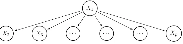
(a) Prec:p=20,d=1 (b) Reca:p=20,d=1 (c) Prec:p=20,d=10 (d) Reca:p=20,d=10
(e) Prec:p=200,d=1 (f) Reca:p=200,d=1 (g) Prec:p=200,d=10 (h) Reca:p=200,d=10
Figure 3: Comparison of the MRS algorithm to the oracle, ODS, GES and MMHC algo-rithms in terms of precision and recall for Poisson SEMs withp ∈ {20,200} and
d∈ {1,10}.
preferred a sparse graph containing only legitimate edges. We acknowledge that the level of sparsity can be adjusted according to the importance of precision or recall.
In Fig. 3, we compare the MRS algorithm to state-of-the-art ODS, GES and MMHC algorithms for graph node size p ={20,200}, varying sample size n∈ {25,50, ...,250} for
d = 1 and n = {100,200, ...,1000} for d = 10, and provide two results: (i) the average precision (# of correctly estimated edges# of estimated edges ); (ii) the average recall (# of correctly estimated edges# of true edges ). As discussed, the both GES and MMHC algorithms only recover the partial graph by leaving some arrows undirected. Therefore, we also provide average precision and recall for the estimated MECs in Fig. 4. Lastly, we provide an oracle, where the true parents of each node are used, while the ordering is estimated via `1-regularized GLM. Hence, we can
see where the errors come from between the ordering estimation or parent selection. We considered more parameters (θjk, n, p, d), but for brevity, we focus on these settings.
As we can see in Fig. 3, the MRS algorithm more accurately recovers the true directed edges as sample size increases. In addition, the MRS algorithm is more precise for small sparse graphs than for large-scale or dense graphs, given the same sample size. Hence it confirms that the MRS algorithm is consistent, and the sample bound n = Ω(d2log9p) depends onp and d.
The MRS algorithm significantly outperforms state-of-the-art GES and MMHC algo-rithms in terms of both precision and recall, on average, except for casesp= 20, d= 1, n≤ 50. It is worth noting that the GES and MMHC algorithms are not consistent, because the recall for any tree graph must be zero in population, whereas the recall from GES and MMHC increases as sample size increases. Hence, we can conclude that the GES and MMHC algorithms find correct directed edges by finding incorrect v-structures. It is an ex-pected result because the comparison methods only work with a non-faithful distribution, which rarely arises in finite sample settings (Uhler et al., 2013).
n 100 200 300 400 500 600 700 800 900 1000
p = 20 199 175 107 64 1 0 0 0 0 0
p = 50 200 200 200 199 192 179 151 140 99 86
Table 1: Number of failures in ODS algorithm implementations from among 200 sets of sam-ples for different node sizesp∈ {20,50}, and sample sizesn∈ {100,200, ...,1000}, when the indegree isd= 5.
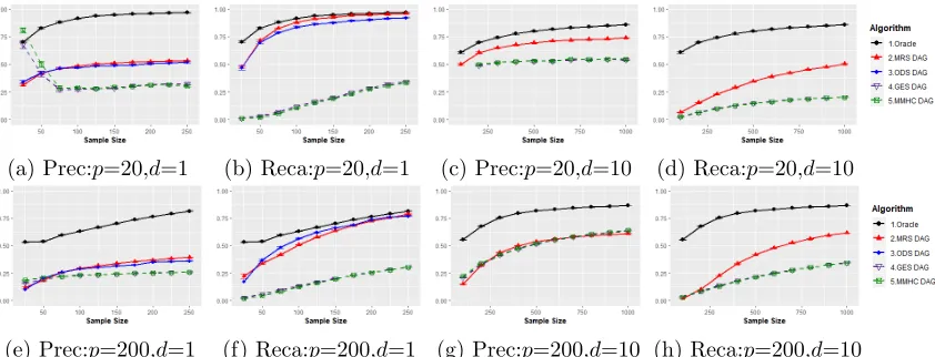
(a) Prec:p=20,d=1 (b) Reca:p=20,d=1 (c) Prec:p=20,d=10 (d) Reca:p=20,d=10
(e) Prec:p=200,d=1 (f) Reca:p=200,d=1 (g) Prec:p=200,d=10 (h) Reca:p=200,d=10
Figure 4: Comparison of the MRS algorithm to the oracle, ODS, GES, and MMHC algo-rithms in terms of the precision and recall for the MECs of Poisson SEMs with
p∈ {20,100} and d∈ {1,10}.
algorithm recovers any Poisson DAG models if the moralized graph is sparse. In other words, the accuracy of the ODS algorithm may be poor for the non-sparse graph. Moreover, the ODS algorithm often fails to be implemented due to a lack of samples for the estimation of conditional variance, that is, Pn
i=11(X (i)
S = x) <2 for all x ∈ XS. Table 1 shows the
number of failures in the ODS algorithm implementations for node size p ∈ {20,50} and sample size n ∈ {100,200, ...,1000} when the indegree is d = 5, and the degree of the moralized graph is at most dm = p−1. It empirically confirms that the ODS algorithm
requires a huge number of samples to be implemented when a true graph is not sparse. Hence, we do not apply the ODS algorithm for the graphs with d = 10. It is consistent with our main result that our method can learn the Poisson SEMs with some hub nodes while the ODS algorithm might not.
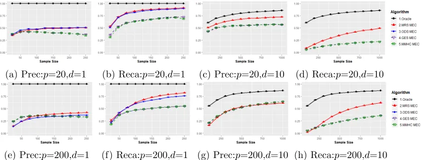
(a) Prec:p=20,d=2 (b) Reca:p=20,d=2 (c) Prec:p=100,d=2 (d) Reca:p=100,d=2
Figure 5: Comparison of the MRS algorithm to the oracle, ODS, GES and MMHC al-gorithms in terms of the precision and recall for Poisson DAG models with
p∈ {20,100},d= 2, and the identity link function.
DAG models where arbitrary link functions are allowed. In addition, the GES and MMHC algorithms apply to more general classes of DAG models.
4.2. Random Poisson DAG Models
When the data are generated by a random Poisson DAG model (2) where gj is not the
standard log link function, our MRS algorithm is not guaranteed to estimate the true directed acyclic graph and its ordering. Hence, an important question is how sensitive our method is to deviations from the link assumption. In this section, we empirically investigate this question.
We generated the 200 samples with the same procedure specified in Section 4.1, but with the indegree constraint d = 2, and except that identity link function gj(η) = η and
the range of parameters was θjk ∈ [−1.5,−0.5]∪[0.5,1.5]. We note that the link function
must be positive, but we allow the negative value of θjk by randomly choosing θj ∈[1,10].
If any Poisson rate parameter is negative, we regenerated the parameters.
In Fig. 5, we compare the MRS to state-of-the-art ODS, GES and MMHC algorithms for varying sample size n∈ {25,50, ...,250}, and node sizep∈ {20,100}. Fig. 5 shows that the MRS algorithm consistently recovers the true graph, and hence, we can see that the MRS algorithm is not so sensitive to deviations from the link assumption. Comparing it to the ODS algorithm, the MRS algorithm shows slightly worse performance because the ODS algorithm is designed to learn general Poisson DAG models with any type of link functions. However, we can see that the MRS algorithm still performs better than the greedy search-based methods in both average precision and recall.
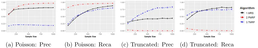
4.3. Random Poisson and Truncated Poisson Markov Random Fields
(a) Poisson: Prec (b) Poisson: Reca (c) Truncated: Prec (d) Truncated: Reca
Figure 6: Comparison of the MRS algorithm to the Poisson MRF learning (PMRF) and truncated Poisson MRF learning (TMRF) algorithms in terms of the precision and recall for undirected edges of random 20-nodes Poisson MRFs and truncated Poisson MRFs withdm = 5, andR= 100.
We generated 100 samples of 20-nodes random Poisson MRF and truncated Poisson MRF with the randomly generated underlying undirected graphs, respectively. For Poisson MRFs, we set the maximum Markov blanket dm = 5 and the non-zero parameters in
Equation (6) was generated uniformly at random in the range θj ∈ [1,2], but we fixed θjk =−0.1 for all j∈V. This is a similar setting used in Yang et al. (2015). For truncated
Poisson MRFs, we set dm = 5, θj = 0, θjk = 0.1, and the truncation level is R = 100,
meaning that all samples are less than 100 (see details in Equation 3 of Yang et al., 2013). In terms of the choice of regularization parameters for the MRS and PMRF algorithms, we used five-fold cross validation as we used in Section 4.1. For the TMRF algorithm, we set the regularization parameters to 0.1 since this value seems to work well.
Fig. 6 compares the MRS algorithm to state-of-the-art PMRF and TMRF algorithms in terms of recovering undirected edges by varying sample sizen∈ {100,200, ...,1000}. For a fair comparison, we used the skeleton of the estimated MEC via the MRS algorithm, because our algorithm returns a DAG. As we can see in Fig. 6, the MRS algorithm consistently finds the true edges from both Poisson MRF and truncated Poisson MRF samples. Hence, we empirically verify that the MRS algorithm can recover some dependence relationships of variables even if samples are from Poisson or truncated Poisson MRFs.
Fig. 6 also shows that the MRS algorithm performs significantly worse than the com-parison PMRF and TMRF algorithm, on average, when samples are from Poisson MRFs and truncated Poisson MRFs, respectively. It is an expected result because the PMRF and TMRF algorithms are for learning Poisson MRFs and truncated MRFs, while our algorithm is for Poisson SEMs. However, it is worth noting that the TMRF algorithm seems not to work on average when samples are from a Poisson MRF in our setting. It is mainly because the TMRF algorithm is for learning truncated Poisson MRFs, not Poisson MRFs. We em-phasize that, in another setting where θj is fixed to 1, the TMRF algorithm works much
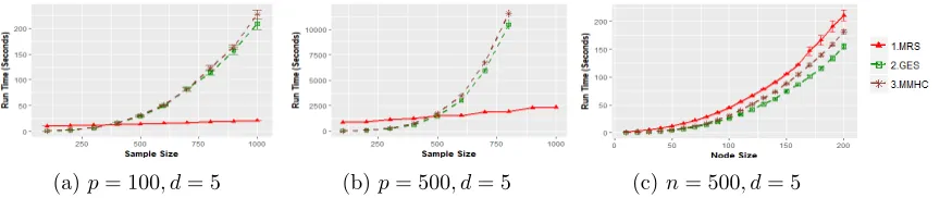
(a)p= 100, d= 5 (b)p= 500, d= 5 (c) n= 500, d= 5
Figure 7: Comparison of the MRS algorithm to the GES and MMHC algorithms in terms of the running time with respect to node sizep and sample size n
4.4. Computational Complexity
Fig. 7 compares the run-time of the MRS, GES, and MMHC algorithms for learning Poisson SEMs with indegreed= 5 by varying sample size n∈ {100,200, ...,1000} with fixed node size p ∈ {100,500}, and varying node size p ∈ {10,20, ...,200} with fixed sample size
n = 500. Fig. 7 supports the worst case computational complexity O(np3) discussed in Section 3.1. In addition, it shows that the MRS algorithm is significantly faster than the greedy search-based GES and MMHC algorithms when a sample size is large (n >500).
5. Real Multivariate Count Data: MLB Statistics
We now apply the MRS algorithm and state-of-the-art ODS and MMHC algorithms to a simple data set that involves multivariate count data that models baseball statistics for Ma-jor League Baseball (MLB) players during the 2003 season. To the best of our knowledge, our MRS algorithm is the only algorithm that provides a reliable and scalable approach to non-sparse DAG learning with multivariate count data although it is under strong as-sumptions. In particular, other approaches, such as PC, MMHC, and approaches based on conditional independence testing, suffer severely from the fact that we are dealing with count variables where the number of discrete states is potentially infinite. In addition, ODS algorithm cannot deal with a non-sparse graph such as a graph containing hub nodes. Lastly, both Poisson MRF and truncated Poisson MRF may provide an extremely compli-cated graph because it connects all pairs of nodes having a common child like a moralized graph.
HBP G
H AB
X2B X3B
CS GIDP RBI SF
R HR SO
SB SH IBB BB
salary
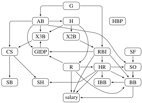
1
Figure 8: MLB player statistics directed graph estimated by the MRS algorithm for Poisson DAG models.
games could be uncertain. Therefore, the data set we considered contained 18 variables and 200 observations.
We assumed each node to a conditional distribution given its parents is Poisson because most MLB statistics, except for salary, reflect the number of successes or attempts that were counted during the season. Hence, we applied the MRS algorithm for Poisson DAG models with leave-one-out cross validation to choose the tuning parameters, and we chose the largest value where mean squared error is within 2.5 standard error of the minimum mean squared error, because we prefer a sparse graph containing only legitimate edges.
Fig. 8 shows the directed graph estimated by our MRS algorithm. The estimated graph reveals clear causal/directional relationships between batting statistics. This makes sense, because players with larger numbers of HR, BB, RBI, and/or R have a better salary. The more games played, or the more batting chances, the higher H, BB, SO, RBI, and other statistics. Moreover, the higher the total number of hits, the more X2Bs, X3Bs, Rs and the fewer SOs. Players with more home runs and base on balls get intentional walks more frequently. Lastly, the more stolen bases are attempted, the more they are caught stealing, because there is no success without failure.
We acknowledge that our proposed DAG model returns many errors due to restrictive assumptions that are not completely satisfied by the real data. However, the benefit is best seen by comparing MRS to other DAG learning approaches and an undirected graphical model for multivariate count data. In particular, we applied Poisson undirected graphical models (Yang et al., 2015) in which `1-regularized Poisson regressions are applied. We
HBP G
H AB
X2B X3B
CS GIDP RBI SF
R HR SO
SB SH IBB BB
salary
1
HBP G
H AB
X2B X3B
CS GIDP RBI SF
R HR SO
SB SH IBB BB
salary
1
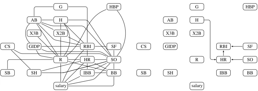
Figure 9: MLB player statistics undirected graph estimated by `1-penalized likelihood re-gression (left) and a directed acyclic graph estimated by the MMHC algorithm (right).
permits negative conditional relationships, whereas most variables are positively correlated. Hence, it may not be useful to understand the relationships between MLB statistics.
We also compared the MMHC algorithm. As discussed, the MMHC algorithm does not guarantee to find a complete directed graph, and prefers a sparser graph when the faithfulness assumption is violated, which often arises in finite sample settings (Uhler et al., 2013). Hence, the estimated directed graph in Fig. 9 (right side) is extremely sparse, with only four directed edges: [H, HR], [SO, HR], [HR, RBI], and [SF, RBI]. Lastly, ODS algorithm failed to be implemented as expected because of some hub nodes such as the number of games, at bats, and runs batted in.
Since our method is the first identifiability result for the strongly correlated count data when variables are directional/causal relationships and there exist hub variables, to the best of our knowledge, our method better identifies the directional/causal relationships between MLB statistics. However, we acknowledge that, like most other DAG-learning approaches, very strong assumptions, such as dependency, incoherence, are required for reliable recovery.
6. Future Works
Several topics remain for future works. Although our assumptions are similar to the assump-tions in the previous works of `1-regularized Poisson regression, our assumptions could be
Acknowledgments
Appendix A. Proof for Proposition 1
Proof For a notational simplicity, we define a moments related function for Poisson,
f(µ) =µ+µ2 forµ >0. Then, for any node j∈V, any non-empty setSj ⊂Nd(j),
E(Xj2 |Sj) = E(E(Xj2 |XPa(j))|Sj) =E(f(E(Xj |XPa(j)))|Sj).
Using the Jensens inequality and f(·) is convex, we have,
E(f(E(Xj |XPa(j)))|Sj)≥f(E(E(Xj |XPa(j))|Sj)) =f(E(Xj |Sj)).
Using the fact thatE(Xj |XPa(j)) =gj(XPa(j)) and it is non-degenerated by definition,
the equality only holds when Sj contains all parents ofj, Pa(j)⊂Sj ⊂Nd(j).
By restating the above inequality, we have,
E(Xj2 |Sj)−E(Xj |Sj)−E(Xj |Sj)2 ≥0.
In addition, by taking the expectations, we have,
E(Xj2)−E E(Xj |XSj) +E(Xj |XSj) 2
≥0.
Since j and Sj are arbitrary, we complete the first part of the proof.
Now, we prove thatE(Xj2)≥E E(Xj |XSj) +E(Xj |XSj) 2
is equivalent toE(Var(E(Xj |
Pa(j))|XSj))≥0. Using the total variance decomposition, we have,
E(Var(Xj |XSj)) =E(E(Var(Xj |XPa(j))|XSj)) +E(Var(E(Xj |XPa(j))|XSj)).
Using the fact that the conditional distribution,Xj |XPa(j), is Poisson where its mean
and variance are equal, we have,
E(Var(E(Xj |XPa(j))|XSj)) =E(Var(Xj |XSj))−E(Xj).
Using the definition of the conditional variance, we have,
E(Var(Xj |XSj))−E(Xj) =E(X 2
j)−E E(Xj |XSj) +E(Xj |XSj) 2
.
Therefore, we complete the proof.
Appendix B. Proof for Theorem 2
Proof Without loss of generality, we assume the true ordering is unique, and π = (π1, ..., πp). For simplicity, we define X1:j = (Xπ1, Xπ2,· · · , Xπj) and X1:0 = ∅. In
ad-dition, we define a moments related function, f(µ) =µ+µ2.
We now prove identifiability of Poisson DAG models using mathematical induction: Step (1) For the first stepπ1, using Proposition 1, we have E(Xπ21) = E(f(E(Xπ1))),
while for any nodej∈V \ {π1}: E(Xj2)>E(f(E(Xj))).
Step (m-1) For the (m−1)th element of the ordering, assume that the first m−1 elements of the ordering and their parents are correctly estimated.
Step (m) Now, we consider the mth element of the causal ordering and its par-ents. It is clear that πm achieves E(Xπ2m) = E(f(E(Xπm | X1:(m−1)))). However, for j ∈ {πm+1,· · ·, πp}, E(Xj2) > E(f(E(Xj | X1:(m−1)))) by Proposition 1. Hence, we can
estimate a true mth component of the orderingπm.
In terms of the parent search, it is clear that by conditional independence relations naturally encoded by factorization (1)E(Xπ2m) =E(f(E(Xπm |X1:(m−1)))) =E(f(E(Xπm | XPa(πm)))).Hence, we can also choose the minimum conditioning set from amongX1:(m−1)
as the parents ofπm such that the above moments relation holds. By mathematical
induc-tion, this completes the proof.
Appendix C. Proof for Theorem 3: Parents Recovery
Proof We provide the proof for Theorem 3 using the primal-dual witness method that is also used many other works (Meinshausen and B¨uhlmann, 2006; Wainwright et al., 2006; Ravikumar et al., 2011; Yang et al., 2015). In this proof, we show in Appendix C, the error probability for the recovery of the parents of a nodeπj from among all the nodes given the
partial ordering (π1, π2, ..., πj−1) via `1-regularized regression. In Appendix D, the error
bounds for the recovery of the ordering both via `1-regularized regression.
Without loss of generality, let the true ordering be π = (1,2, ..., p), and hence, π1:j =
(π1, π2, ..., πj) = (1,2, ..., j). For ease of notation, [·]kand [·]Sdenote parameters
correspond-ing to variable Xk and random vector XS, respectively. In order to make the arguments
easier to understand, we restate the negative log likelihood (10) and related arguments. First, we define a new parameter vectorθSj ∈R
|Sj|without parameterθ
j corresponding
to the node j since the node j is not penalized in regression problem (9). Then, the conditional negative log-likelihood of the GLM forXj given XSj can be written as:
`Sj
j (θSj;X
1:n) := 1 n
n
X
i=1
−Xj(i)hθSj, X (i)
Sji+ exp hθSj, X (i) Sji
, (13)
whereh·,·iis an inner product. We also define θS∗
j ∈R
|Sj|for Equation (11):
θ∗Sj := arg min
θ∈R|Sj|
E −Xj(hθ, XSji) + exp(hθ, XSji)
. (14)
We define a set non-zero elements index of θ∗S
j as in Equation (12), Tj := {k ∈ Sj |
[θS∗j]k6= 0}where θS∗j is in Equation (14).
The main goal of the proof is to find the unique minimizer of the following convex problem:
b
θSj := arg min θ∈R|Sj|
Lj(θ, λj) = arg min θ∈R|Sj|
{`Sj
By setting the sub-differential to 0,θbSj satisfies the following condition:
5θLSj
j (θbSj, λj) =5θ`
Sj
j (θbSj;X1:n) +λjZb
Sj
j = 0 (16)
whereZb
Sj
j ∈R|Sj| and [Zb
Sj
j ]t= sign([bθSj]t) if t∈Tj, otherwise [Zb
Sj j ]t<1.
Lemma 4 directly follows from the prior work (Yang et al., 2015), where each node’s conditional distribution is in the form of a generalized linear model.
Lemma 4 (Uniqueness of Solution, Lemma 8 in Yang et al., 2015) Suppose that
|[Zb
Sj
j ]t|<1 for t /∈Tj in Equation (16). Then, the solution θbSj of Equation (15) satisfies
[bθSj]t= 0for allt /∈Tj. Furthermore, if the sub-matrix of Hessian matrixQ
Sj
TjTj is invertible, thenθbSj is unique.
The remainder of the proof is to show|[Zb
Sj
j ]t|<1 for allt /∈Tj. Note that the restricted
solution in Equation (22) is (θeSj,Ze
Sj
j ) and the unrestricted solution in Equation (15) is
(θbSj,Zb
Sj
j ). Equation (16) with the dual solution can be represented by
52`Sjj(θ∗Sj;X1:n)(θeSj−θS∗
j) =−λjZe Sj j −W
Sj j +R
Sj
j (17)
where
(a) WSj
j is the sample score function:
WSj
j :=− 5`j(θ∗Sj;X
1:n). (18)
(b) RSjj = (RjkSj)k∈Sj andR Sj
jk is the remainder term by applying the coordinate-wise mean
value theorem:
RSjkj := [52`Sjj(θS∗j;X1:n)− 52`Sjj(¯θSj;X 1:n)]T
k(θeSj−θ∗S
j). (19)
Here ¯θSj is a vector on the line between θeSj and θ ∗
Sj, and [·] T
k is the row of a matrix
corresponding to variable Xk.
Then, the following proposition provides a sufficient condition to control Ze
Sj j .
Proposition 5 If max(kWSj
j k∞,kR Sj j k∞)≤
λjα
4(2−α), then |[Ze
Sj
j ]t|<1 for allt /∈Tj.
Next, we introduce the following three lemmas under Assumptions 1, 2, and 3 to show that conditions in Proposition 5 hold. For ease of notation, letη= max{n, p},θeS = [θeS
j]Tj,
e
ZS = [Ze
Sj
j ]Tj,θeSc = [θeSj]Sj\Tj, and ZeSc = [Ze Sj j ]Sj\Tj.
Lemma 6 For any Sj ∈ {π1, π1:2, ..., π1:j−1} and λj ≥ 4C 2 x √
2(2−α) α
log2η
κ1(n,p) for some α ∈
(0,1],
P kW Sj j k∞ λj
≤ α
4(2−α)
!
≥1−2d·exp
− n
κ1(n, p)2
.
Lemma 7 Suppose that for all Sj ∈ {π1, π1:2, ..., π1:j−1}, kWjSjk∞ ≤ λ4j. Then, for λj ≤ ρ2
min 10C2
xρmaxdlog2η,
keθS−θS∗k2 ≤
5
ρmin
√
dλj
Lemma 8 Suppose that for all Sj ∈ {π1, π1:2, ..., π1:j−1}, kWjSjk∞ ≤ λ4j. Then, for λj ≤ αρ2
min 100C2
x(2−α)ρmaxdlog2η andα∈(0,1],
kRSj j k∞ λj
≤ α
4(2−α)
The rest of the proof is straightforward using Lemmas 6, 7, and 8. Consider the choice of regularization parameterλj0= 4
√ 2C2
x(2−α) α
log2η
κ1(n,p), whereκ1(n, p)≥ 4√2C4
x·102(2−α)2 α2
ρmax ρ2
min
dlog4η
ensuring that 4Cx2 √
2(2−α) α
log2η
κ1(n,p) ≤ λj0 ≤
αρ2 min 102C2
x(2−α)ρmaxdlog2η for any α = (0,1]. Hence, if
we set κ1(n, p) = Cmaxdlog4η where Cmax = 4
√ 2·102C4
x·(2−α)2 α2
ρmax ρ2
min
, then all conditions for Lemma 6, 7, and 8 are satisfied. Therefore,
kZeSck∞≤(1−α) + (2−α)
"
kWSj j k∞ λj
+kR
Sj j k∞ λj
#
≤(1−α) + α 4 +
α
4 <1, (20)
with a probability of at least 1−2d·exp
−κ1(n,pn )2
= 1−2d·exp
− n
C2
maxd2log8η
.
Proposition 9 Suppose that, for any j ∈ V, partial ordering (π1, ..., πj) is correctly esti-mated. If mint∈S[θ∗S]t≥ ρ10min
√
d λj for all j∈V,
supp(θbSj) =Pa(j).
Proposition 9 guarantees that `1-regularized likelihood regression recovers the parents for each node with a high probability. Since there are p regression problems, for any
> 0, there exists a positive constant C > 0 such that if n ≥ C(κ1(n, p)2logp) for κ1(n, p)≥Cmaxdlog4η,
P(Gb=G)≥2dp·exp
− n
κ1(n, p)2
≥1−2dp·exp (−Clogp)≥1−.
Appendix D. Proof for Theorem 3: Ordering Recovery
= (X1, X2, ..., Xj) andX1:0 =∅. We restate the moments ratio scores for a nodek and the jth element of the ordering:
S(j, k) := E(X
2 k)
E(f(E(Xk|X1:(j−1))))
and S(bj, k) :=
b
E(Xk2)
b
E(f(E(b Xk|X
b
π1:(j−1)))) ,
wheref(µ) :=µ+µ2,E(Xk|XSk) = exp(θ ∗ k+
P
t∈Skθ ∗
ktXt), andE(b Xk|XSk) = exp(ˆθk+ P
t∈Sk
ˆ
θktXt) whereθS∗k = (θk∗, θ∗kt) and ˆθSk = (ˆθk,θˆkt) are the solutions of the problem (11)
and of the `1-regularized GLM (9), respectively. In addition, we use the unbiased method-of-moment estimator for a marginal expectation, Eb(Xk2) = 1n
Pn
i=1(X (i)
k )2 and Eb(f(Eb(Xk|
XS))) = n1 Pni=1f(exp(ˆθk+
P
t∈Sk
ˆ
θktX (i) t )).
We define the following necessary events: For each nodej∈V,Sj ∈ {π1, π1:2, ..., π1:(j−1)}
and any 1 >0;
ζ1 :=
max
j=1,...,p−1k=maxj,...,p
S(j, πk)−Sb(j, πk) > Mmin 2 ,
ζ2 :=
max
j∈V
Eb(X
2
j)−E(Xj2)
< 1
,
ζ3 :=
max
j∈V
Eb
fEb(Xj |XSj)
−EfEb(Xj |XSj)
< 1
,
ζ4 :=
max
j∈V
E f b
E(Xj |XSj)
−E f E(Xj |XSj)
< 1
.
We begin by proving that our algorithm recovers the ordering of a Poisson SEM in the high-dimensional setting. The probability that ordering is correctly estimated from our method can be written as
P(bπ=π)
=P
b
S(1, π1)< min
j=2,...,pS(1b , πj),S(2b , π2)<j=3min,...,pS(2b , πj), ...,S(bp−1, πp−1)<S(b p−1, πp)
=P
min
j=1,...,p−1k=jmin+1,...,p
b
S(j, πk)−S(bj, πj)>0
=P
min
j=1,...,p−1 k=j+1,...,p
n
S(j, πk)− S(j, πj)
−S(j, πk)−S(bj, πk)
+
S(j, πj)−S(b j, πj) o >0 ≥P min
j=1,...,p−1 k=j+1,...,p
{(S(j, πk)− S(j, πj))}> Mmin, and max j=1,...,p−1
k=j,...,p
S(j, πk)−S(bj, πk) < Mmin 2 .
The first term in the above probability is always satisfied because S(j, πk)− S(j, πj)>
ordering is correctly estimated using our method is reduced to
P(bπ=π) ≥ P
max
j=1,...,p−1k=maxj,...,p
S(j, πk)−S(bj, πk) <
Mmin
2
= 1−P(ζ1)
= 1−P(ζ1 |ζ2, ζ3, ζ4)P(ζ2, ζ3, ζ4)−P(ζ1|(ζ2, ζ3, ζ4)c)P((ζ2, ζ3, ζ4)c) ≥ 1−P(ζ1 |ζ2, ζ3, ζ4)−P((ζ2, ζ3, ζ4)c)
≥ 1−P(ζ1 |ζ2, ζ3, ζ4)
| {z }
Lem10
−P(ζ2c)−P(ζ3c)−P(ζ4c)
| {z }
Lem11
. (21)
Next, we introduce the following two lemmas to show the lower bound of the probability in (21) as a function of the triple (n, p, d):
Lemma 10 Given the sets ζ2, ζ3, ζ4 and under Assumption 4, P(ζ1 | ζ2, ζ3, ζ4) = 0 if for some small 1 such that for any Sj ∈ {π1, π1:2, ..., π1:(j−1)},
1 <min
(
E(Xj2)Mmin
2(Mmin+ 3)(Mmin+ 1) ,Mmin
6
E(f(E(Xj |XSj))) 2
E(Xj2)
)
,
where f(µ) =µ+µ2.
The condition in Lemma 10 implies that if 1 is sufficiently small, the estimated score is
close to the true score value.
The second lemma shows the error bound for the consistency of the estimators.
Lemma 11 For any 1 >0 and
(i) For ζ2, P(ζ2c)≤1−2·p·exp
n
− n21 2C2
xlog2η
o
.
(ii) For ζ3, there exist some positive constantsCmax and Dmax such that P(ζ3c)≤1−2·p·d· exp− n
κ1(n,p)2
−2·p·expn− n21 Dmaxlog4η
o
.
where κ1(n, p)≥Cmaxdlog4η. (iii) For ζ4, P(ζ4c) = 0.
Therefore, we complete the proof: our method recovers the true ordering at least of
P(bπ=π) ≥ 1−C1p·d·exp
−C2 n κ1(n, p)2
.