No-Regret Bayesian Optimization with
Unknown Hyperparameters
Felix Berkenkamp [email protected]
Department of Computer Science ETH Zurich
Zurich, Switzerland
Angela P. Schoellig [email protected]
Institute for Aerospace Studies University of Toronto
Toronto, Canada
Andreas Krause [email protected]
Department of Computer Science ETH Zurich
Zurich, Switzerland
Editor:Bayesian Optimization Special Issue
Abstract
Bayesian optimization (BO) based on Gaussian process models is a powerful paradigm to optimize black-box functions that are expensive to evaluate. While several BO algorithms provably converge to the global optimum of the unknown function, they assume that the hyperparameters of the kernel are known in advance. This is not the case in practice and misspecification often causes these algorithms to converge to poor local optima. In this paper, we present the first BO algorithm that is provably no-regret and converges to the optimum without knowledge of the hyperparameters. During optimization we slowly adapt the hyperparameters of stationary kernels and thereby expand the associated function class over time, so that the BO algorithm considers more complex function candidates. Based on the theoretical insights, we propose several practical algorithms that achieve the empir-ical sample efficiency of BO with online hyperparameter estimation, but retain theoretempir-ical convergence guarantees. We evaluate our method on several benchmark problems.
Keywords: Bayesian optimization, Unknown hyperparameters, Reproducing kernel Hilbert space (RKHS), Bandits, No regret
1. Introduction
The performance of machine learning algorithms often critically depends on the choice of tuning inputs, e.g., learning rates or regularization constants. Picking these correctly is a key challenge. Traditionally, these inputs are optimized using grid or random search (Bergstra and Bengio, 2012). However, as data sets become larger the computation time required to train a single model increases, which renders these approaches less applicable. Bayesian optimization (BO, Mockus (2012)) is an alternative method that provably determines good inputs within few evaluations of the underlying objective function. BO methods construct a statistical model of the underlying objective function and use it to evaluate inputs that
c
are informative about the optimum. However, the theoretical guarantees, empirical perfor-mance, and data efficiency of BO algorithms critically depend on their own choice of hyper-parameters and, in particular, on the prior distribution over the function space. Thus, we effectively shift the problem of tuning inputs one level up, to the tuning of hyperparameters of the BO algorithm.
In this paper, we use a Gaussian processes (GP, Rasmussen and Williams (2006)) for the statistical model. We present the first BO algorithm that does not require knowledge about the hyperparameters of the GP’s stationary kernel and provably converges to the global optimum. To this end, we adapt the hyperparameters of the kernel and our BO algorithm, so that the associated function space grows over time. The resulting algorithm provably converges to the global optimum and retains theoretical convergence guarantees, even when combined with online estimation of hyperparameters.
Related work General BO has received a lot of attention in recent years. Typically, BO algorithms suggest inputs to evaluate by maximizing an acqusition function that mea-sures informativeness about the optimum. Classical acquisition functions are the expected improvement over the best known function value encountered so far given the GP distribu-tion (Mockus et al., 1978) and the Upper Confidence Bound algorithm, GP-UCB, which
applies the ‘optimism in the face of uncertainty’ principle. The latter is shown to provably converge by Srinivas et al. (2012). Durand et al. (2018) extend this framework to the case of unknown measurement noise. A related method is truncated variance reduction by Bo-gunovic et al. (2016), which considers the reduction in uncertainty at candidate locations for the optimum. Hennig and Schuler (2012) propose entropy search, which approximates the distribution of the optimum of the objective function and uses the reduction of the entropy in this distribution as an acquisition function. Alternative information-theoretic methods are proposed by Hern´andez-Lobato et al. (2014); Wang and Jegelka (2017); Ru et al. (2018). Other alternatives are theknowledge gradient (Frazier et al., 2009), which is one-step Bayes optimal, and information directed sampling by Russo and Van Roy (2014), which considers a tradeoff between regret and information gained when evaluating an input. Kirschner and Krause (2018) extend the latter framework to heteroscedastic noise.
These BO methods have also been successful empirically. In machine learning, they are used to optimize the performance of learning methods (Brochu et al., 2010; Snoek et al., 2012). BO is also applicable more broadly; for example, in reinforcement learning to opti-mize a parametric policy for a robot (Calandra et al., 2014; Lizotte et al., 2007; Berkenkamp et al., 2016) or in control to optimize the energy output of a power plant (Abdelrahman et al., 2016). It also forms the backbone of Google vizier, a service for tuning black-box functions (Golovin et al., 2017).
Freitas (2014) analyze this setting when a lower bound on the kernel lengthscales is known
a priori. They decrease the lengthscales over time and bound the regret in terms of the known lower-bound on the lengthscales. Empirically, similar heuristics are used by Wang et al. (2016); Wabersich and Toussaint (2016). In contrast, this paper considers the case where the hyperparameters are not known. Moreover, the scaling of the hyperparameters in the previous two papers did not depend on the dimensionality of the problem, which can cause the function space to increase too quickly.
Considering larger function classes as more data becomes available is the core idea behind structural risk minimization (Vapnik, 1992) in statistical learning theory. However, there data is assumed to be sampled independently and identically distributed. This is not the case in BO, where new data is generated actively based on past information.
Our contribution In this paper, we present AdaptiveGP-UCB (A-GP-UCB), the first
algorithm that provably converges to the globally optimal inputs when BO hyperparameters areunknown. Our method expands the function class encoded in the model over time, but does so slowly enough to ensure sublinear regret and convergence to the optimum. Based on the theoretical insights, we propose practical variants of the algorithm with guaranteed convergence. Since our method can be used as an add-on module to existing algorithms with hyperparameter estimation, it achieves similar performance empirically, but avoids local optima when hyperparameters are misspecified. In summary, we:
• Provide theoretical convergence guarantees for BO with unknown hyperparameters; • Propose several practical algorithms based on the theoretical insights;
• Evaluate the performance in practice and show that our method retains the empirical performance of heuristic methods based on online hyperparameter estimation, but leads to significantly improved performance when the model is misspecified initially.
The remainder of the paper is structured as follows. We state the problem in Sec. 2 and provide relevant background material in Sec. 3. We derive our main theoretical result in Sec. 4 and use insights gained from the theory to propose practical algorithms. We evaluate these algorithms experimentally in Sec. 5 and draw conclusions in Sec. 6. The technical details of the proofs are given in the appendix.
2. Problem Statement
In general, BO considers global optimization problems of the form
x∗ = argmax
x∈D
f(x), (1)
whereD ⊂Rdis a compact domain over which we want to optimize inputsx, andf:D →R
Regret We aim to construct a sequence of input evaluationsxt, that eventually maximizes
the function value f(xt). One natural way to prove this convergence is to show that an
algorithm has sublinear regret. The instantaneous regret at iteration t is defined as rt =
maxx∈Df(x)−f(xt)≥0, which is the loss incurred by evaluating the function atxtinstead
of at the a priori unknown optimal inputs. The cumulative regret is defined as RT =
P
0<t≤T rt, the sum of regrets incurred over T steps. If we can show that the cumulative
regret is sublinear for a given algorithm, that is, limt→∞Rt/ t = 0, then eventually the
algorithm evaluates the function at inputs that lead to close-to-optimal function values most of the time. We say that such an algorithm has no-regret. Intuitively, if the average regret approaches zero then, on average, the instantaneous regret must approach zero too, sincert
is strictly positive. This implies that there exists at >0 such thatf(xt) is arbitrarily close
to f(x∗) and the algorithm converges. Thus, we aim to design an optimization algorithm that has sublinear regret.
Regularity assumptions Without further assumptions, it is impossible to achieve sub-linear regret on (1). In the worst case, f could be discontinuous at every input inD. To make the optimization problem in (1) tractable, we make regularity assumptions about f. In particular, we assume that the functionf has low complexity, as measured by the norm in a reproducing kernel Hilbert space (RKHS, Christmann and Steinwart (2008)). An RKHS Hk contains well-behaved functions of the form f(x) = Pi≥0αik(x,xi), for given
representer points xi ∈ Rd and weights αi ∈ R that decay sufficiently quickly. The
ker-nel k(·,·) determines the roughness and size of the function space and the induced RKHS norm kfkk =
p
hf, fi measures the complexity of a function f ∈ Hk with respect to the
kernel.
In the following, we assume that f in (1) has bounded RKHS norm kfkkθ ≤ B with
respect to a kernel kθ that is parameterized by hyperparameters θ. We write Hθ for the
corresponding RKHS,Hkθ. For knownBandθ, no-regret BO algorithms for (1) are known,
e.g.,GP-UCB(Srinivas et al., 2012). In practice, these hyperparameters need to be tuned.
In this paper, we consider the case where θ and B are unknown. We focus on stationary kernels, which measure similarity based on the distance of inputs,k(x,x0) =k(x−x0). The most commonly used hyperparameters for these kernels are the lengthscalesθ∈Rd, which
scale the inputs to the kernel in order to account for different magnitudes in the different components ofxand effects on the output value. That is, we scale the differencex−x0 by the lengthscalesθ,
kθ(x,x0) =k
[x]1−[x0]1 [θ]1
, . . . , [x]d−[x
0]
d
[θ]d
, (2)
where [x]i denotes the ith element of x. Typically, these kernels assign larger similarity
scores to inputs when the scaled distance between these two inputs is small. Another common hyperparameter is the prior variance of the kernel, a multiplicative constant that determines the magnitude of the kernel. We assumek(x,x) = 1 for allx∈ D without loss of generality, as any multiplicative scaling can be absorbed by the norm boundB.
In summary, our goal is to efficiently solve (1) via a BO algorithm with sublinear re-gret, where f lies in some RKHS Hθ, but neither the hyperparameters θ nor the
3. Background
In this section, we review Gaussian processes (GPs) and Bayesian optimization (BO).
3.1. Gaussian processes (GP)
Based on the assumptions in Sec. 2, we can use GPs to infer confidence intervals onf. The goal of GP inference is to infer a posterior distribution over the nonlinear mapf(x) :D→R
from an input vector x∈D to the function valuef(x). This is accomplished by assuming that the function valuesf(x), associated with different values ofx, are random variables and that any finite number of these random variables have a joint Gaussian distribution (Ras-mussen and Williams, 2006). A GP distribution is parameterized by a prior mean function and a covariance function or kernel k(x,x0), which defines the covariance of any two func-tion values f(x) and f(x0) for x,x0 ∈D. In this work, the mean is assumed to be zero without loss of generality. The choice of kernel function is problem-dependent and encodes assumptions about the unknown function.
We can condition a GP(0, k(x,x0)) on a set of t past observations yt= (y1, . . . , yt)
at inputs At = {x1, . . . ,xt} in order to obtain a posterior distribution on f(x) for any
inputx∈D. The GP model assumes that observations are noisy measurements of the true function value,yt=f(xt) +ωt, whereωt∼ N(0, σ2). The posterior distribution is again a
GP(µt(x), kt(x,x0)) with meanµt, covariancekt, and varianceσt, where
µt(x) =kt(x)(Kt+Iσ2)−1yt, (3)
kt(x,x0) =k(x,x0)−kt(x)(Kt+Iσ2)−1kTt(x0), (4)
σ2t(x) =kt(x,x). (5)
The covariance matrix Kt∈Rt×t has entries [Kt](i,j)=k(xi,xj), i, j∈ {1, . . . , t}, and the
vectorkt(x) =
k(x,x1), . . . , k(x,xt)
contains the covariances between the inputxand the observed data points in At. The identity matrix is denoted byIt∈Rt×t.
3.2. Learning RKHS functions with GPs
The GP framework uses a statistical model that makes different assumptions from the ones made aboutf in Sec. 2. In particular, we assume a different noise model, and samples from a GP(0, k(x,x0)) are rougher than RKHS funtions and are not contained in Hk. However,
GPs and RKHS functions are closely related (Kanagawa et al., 2018) and it is possible to use GP models to infer reliable confidence intervals onf in (1).
Lemma 1 (Abbasi-Yadkori (2012); Chowdhury and Gopalan (2017)) Assume that f has bounded RKHS norm kfkk ≤ B and that measurements are corrupted by
σ-sub-Gaussian noise. If β1t/2 =B+ 4σpI(yt;f) + 1 + ln(1/δ), then for all x∈D and t≥0 it
holds jointly with probability at least 1−δ that|f(x)−µt(x)| ≤βt1/2σt(x).
Lemma 1 implies that, with high probability, the true functionf is contained in the confi-dence intervals induced by the posterior GP distribution that uses the kernelkfrom Lemma 1 as a covariance function, scaled by an appropriate factorβt. Here,I(yt;f) denotes the
GP models this quantity only depends on the inputs xt and not the corresponding
mea-surement yt. Specifically, for a given set of measurementsyA at inputsx∈ A, the mutual information is given by
I(yA;f) = 0.5 log|I+σ−2KA|, (6)
where KA is the kernel matrix [k(x,x0)]x,x0∈A and | · | is the determinant. Intuitively, the mutual information measures how informative the collected samples yA are about the functionf. If the function values are independent of each other under the GP prior, they will provide large amounts of new information. However, if measurements are taken close to each other as measured by the kernel, they are correlated under the GP prior and provide less information.
3.3. Bayesian Optimization (BO)
BO aims to find the global maximum of an unknown function (Mockus, 2012). The frame-work assumes that evaluating the function is expensive in terms of time required or monetary costs, while other computational resources are comparatively inexpensive. In general, BO methods model the objective function f with a statistical model and use it to determine informative sample locations. A popular approach is to model the underlying function with a GP, see Sec. 3.1. GP-based BO methods use the posterior mean and variance predictions in (3) and (5) to compute the next sample location.
One commonly used algorithm is the GP-UCB algorithm by Srinivas et al. (2012). It
uses confidence intervals on the function f, e.g., from Lemma 1, in order to select as next input the point with the largest plasuble function value according to the model,
xt+1= argmax
x∈D
µt(x) +β
1/2
t σt(x). (7)
Intuitively, (7) selects new evaluation points at locations where the upper bound of the confidence interval of the GP estimate is maximal. Repeatedly evaluating the function f
at inputs xt+1 given by (7) improves the mean estimate of the underlying function and decreases the uncertainty at candidate locations for the maximum, so that the global max-imum is provably found eventually (Srinivas et al., 2012). While (7) is also an optimization problem, it only depends on the GP model of f and solving it therefore does not require any expensive evaluations off.
Regret bounds Srinivas et al. (2012) show that theGP-UCBalgorithm has cumulative
regret Rt = O(√tβtγt) for all t ≥ 1 with the same (1−δ) probability as the confidence
intervals, e.g., in Lemma 1, hold. Hereγtis the largest amount of mutual information that
could be obtained by any algorithm from at mostt measurements,
γt= max
A⊂D,|A|≤tI(yA;f). (8)
We refer to γt as the information capacity, since it can be interpreted as a measure of
complexity of the function class associated with a GP prior. It was shown by Srinivas et al. (2012) that γt has a sublinear dependence on t for many commonly used kernels such as
the Gaussian kernel. As a result, Rt has a sublinear dependence ontso thatRt/t→0 and
−1 0 1 Parametersx
−1 0 1
(a) Sample from GP prior.
−1 0 1
Parametersx
−1 0
1 truef(x)
(b) GP estimate (RKHS).
0 1 2
Lengthscaleθ
0.0 0.5 1.0
p
(
θ
|
At
,
yt
)
Prior Posterior
samples
θMAP
Trueθ
(c) Lengthscale distribution.
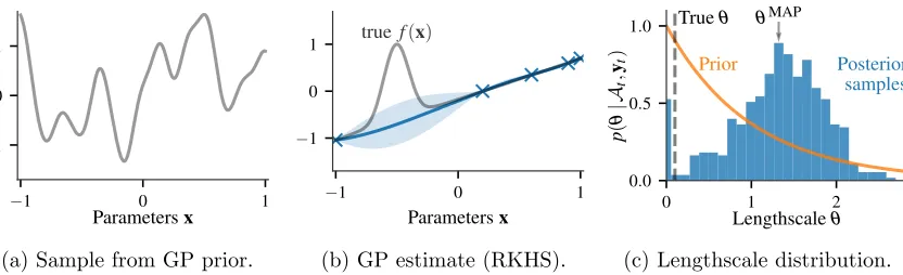
Figure 1: A sample from the GP prior in Fig. 1a typically varies at a consistent rate over the input space. However, RKHS functions with the same kernel may be less consistent and can have bumps, as in Fig. 1b (gray). As a result, inferring the posterior lengthscales based on measurements (blue crosses in Fig. 1b) can lead to erroneous results. In Fig. 1c, most of the probability mass of the posterior lengthscales has concentrated around large lengthscales that encode smooth functions. Consequently, the GP’s 2σ confidence intervals in Fig. 1b (blue shaded) based on the posterior samples do not contain the true function.
were extended to Thompson sampling, an algorithm that uses samples from the posterior GP as the acquisition function, by Chowdhury and Gopalan (2017).
Online hyperparameter estimation In the previous section, we have seen that the GP-UCB algorithm provably converges. However, it requires access to a RKHS norm bound
kfkθ ≤B under the correct kernel hyperparameters θ in order to construct reliable
confi-dence intervals using Lemma 1. In practice, these are unknown and have to be estimated online, e.g., based on a prior distribution placed on θ. Unfortunately, it is well-known that online estimation of the inputs, be it via maximum a posteriori (MAP) or sampling methods, does not always converge to the optimum (Bull, 2011). The problem does not primarily lie with the inference scheme, but rather with the assumptions made by the GP. In particular, typical samples drawn from a GP with a stationary kernel tend to have a similar rate of change throughout the input space, see Fig. 1a. In contrast, the functions inside the RKHS, as specified in Sec. 2, can have different rates of change and are thus im-probable under the GP prior. For example, the grey function in Fig. 1b is almost linear but has one bump that defines the global maximum, which makes this function an improbable sample under the GP prior even though it belongs to the RKHS induced by the same kernel. This property of GPs with stationary kernels means that, for inference, it is sufficient to estimate the lengthscales in a small part of the state-space in order to make statements about the function space globally. This is illustrated in Fig. 1c, where we show samples from the posterior distribution over the lengthscales based on the measurements obtained from theGP-UCB algorithm in Fig. 1b (blue crosses). Even though the prior distribution
Parametersx
next evaluation truef(x)
(a) Stuck in local optimum.
Parametersx
(b) Expanding the function class.
Parametersx
(c) Global optimum found.
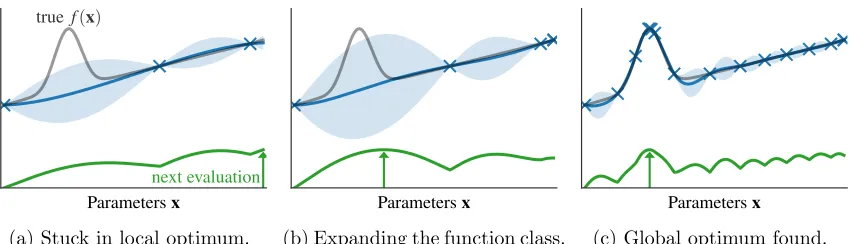
Figure 2: BO algorithms get stuck in local optima when the hyperpararameters of the model are misspecified. In Fig. 2a, the true function is not contained within the GP’s confidence intervals (blue shaded), so that GP-UCB only collects data at the local optimum on the
right (green arrow), see also Fig. 1. Our method expands the function class over time by scaling the hyperparameters, which encourages additional exploration in Fig. 2b. The function class grows slowly enough, so that the global optimum is provably found in Fig. 2c.
the probabilistic model that we have specified based on the stationary kernel, which does not consider functions with different rates of change to be likely.
4. The Adaptive GP-UCB Algorithm
In this section, we extend the GP-UCB algorithm to the case where neither the norm
bound B nor the lengthscales θ are known. In this case, it is always possible that the local optimum is defined by a local bump based on a kernel with small lengthscales, which has not been encountered by the data points as in Fig. 1b. The only solution to avoid this problem is to keep exploring to eventually cover the input spaceD(Bull, 2011). We consider expanding the function space associated with the hyperparameters slowly over time, so that we obtain sublinear regret once the true function class has been identified. Intuitively, this can help BO algorithms avoid premature convergence to local optima caused by misspecified hyperparametersθand B. For example, in Fig. 2a, theGP-UCBalgorithm has converged
to a local maximum. By decreasing the lengthscales, we increase the underlying function class, which means that the GP confidence intervals on the function increase. This enables
GP-UCBto explore further so that the global optimum is found, as shown in Fig. 2c.
Specifically, we start with an initial guess θ0 and B0 for the lengthscales and norm bound onf, respectively. Over the iterations, we scale down the lengthscales and scale up the norm bound,
θt=
1
g(t)θ0, Bt=b(t)g(t)
dB
0, (9)
where g:N → R>0 and b:N → R>0 with b(0) = g(0) = 1 are functions that can addi-tionally depend on the data collected up to iteration t, At and yt. As g(t) increases, the
(a) Scaling of the norm bound. (b) Cumulative regret with scaling.
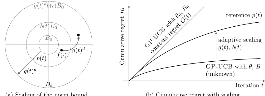
Figure 3: The function f in Fig. 3a has RKHS norm kfkθ0 > B0. To account for this, we
expand the norm ball by b(t) over time. When we scale down the lengthscales byg(t), the norm off in the resulting RKHS is larger, see Lemma 2. We account for this when defining the norm ball Bt in (9). In Fig. 3b, the GP-UCB algorithm based on the misspecified
hyperparameters B0 and θ0 does not converge (constant regret). Our method scales the lengthscales and norm bound byg(t) andb(t), so that we eventually capture the true model. Scaling the hyperparameters beyond the true ones leads to additional exploration and thus larger cumulative regret than GP-UCB with the true, unknown hyperparameters θ and B. However, as long as the cumulative regret is upper bounded by a sublinear function p, ultimately the A-GP-UCB algorithm converges to the global optimum.
Lemma 2 (Bull, 2011, Lemma 4) If f ∈ Hθ, then f ∈ Hθ0 for all 0< θ0 ≤θ, and
kfk2Hθ0 ≤
d
Y
i=1 [θ]i
[θ0]
i
!
kfk2Hθ. (10)
Lemma 2 states that when decreasing the lengthscales θ, the resulting function space con-tains the previous one. Thus, asg(t) increases we consider larger RKHS spaces as candidate spaces for the function f. In addition, as we increase b(t), we consider larger norm balls within the function space Hθt, which corresponds to more complex functions. However,
it follows from (10) that, as we increase g(t), we also increase the norm of any existing function in Hθ0 by at most a factor of g(t)
d. This is illustrated in Fig. 3a: as we scale
up the norm ball to b(t)B0, we capture f under the initial lengthscales θ0. However, by shortening the lengthscales by g(t), the function f has a larger norm in the new function spaceHθt =Hθ0/g(t). We account for this through the additional scaling factorg(t)
d in the
norm boundBtin (9).
Theoretical analysis Based on the previous derivations together with Lemma 2, it is clear that, ifg(t) andb(t) are monotonically increasing functions andf ∈ Hθt∗ withkfkθt∗ ≤
Based on this insight, we proposeA-GP-UCBin Algorithm 1. At iterationt,A-GP-UCB
sets the GP lengthscales toθtand selects new inputsxt+1similar to theGP-UCBalgorithm,
but based on the norm bound Bt. We extend the analysis of GP-UCB and Lemma 1 to
obtain our main result.
Theorem 1 Assume that f has bounded RKHS norm kfk2
kθ ≤ B in a RKHS that is
parametrized by a stationary kernel kθ(x,x0) with unknown lengthscales θ. Based on an
initial guess, θ0 and B0, define monotonically increasing functions g(t) > 0 and b(t) > 0
and run A-GP-UCBwithβt1/2 =b(t)g(t)dB0+4σ
p
Iθt(yt;f) + 1 + ln(1/δ) and GP
length-scales θt=θ0/g(t). Then, with probability at least(1−δ), we obtain a regret bound of
Rt≤2Bmax
g−1
max
i
[θ0]i
[θ]i
, b−1
B
B0
+pC1tβtIθt(yt;f), (11)
where Iθt is the mutual information in (6) based on the GP model with lengthscales θt
and C1 = 8/log(1 +σ−2).
The proof is given in the appendix. Intuitively, the regret bound in (11) splits the run of the algorithm into two distinct phases. In the first one, either the RKHS spaceHθt(D) or
the norm bound Bt are too small to contain the true function f. Thus, the GP confidence
intervals scaled by βt1/2 do not necessarily contain the true function f, as in Fig. 1b. In these iterations, we obtain constant regret that is bounded by 2B, since kfk∞ ≤ kfkθ ≤
B. After both g and b have grown sufficiently in order for the considered function space to contain the true function, the confidence bounds are reliable and we can apply the theoretical results of the GP-UCB algorithm. This is illustrated in Fig. 3b: If the initial
hyperparametersθ0 and B0 are misspecified, the confidence intervals do not containf and
GP-UCBdoes not converge. We avoid this problem by increasingb(t) andg(t) over time,
so that we eventually contain f in our function class. However, increasing the norm ball and decreasing the lengthscales beyond the true ones causes additional exploration and thus additional cumulative regret relative toGP-UCBwith the true, unknown hyperparameters.
This additional regret represents the cost of not knowing the hyperparameters in advance. As long as the overall regret remains bounded by a sublinear function p(t), our method eventually converges to the global optimum. The regret bound in (11) depends on the true hyperparameters θ and B. However, the algorithm does not depend on them. Theorem 1 provides an instance-specific bound, since the mutual information depends on the inputs inAt. One can obtain a worst-case upper bound by boundingIθt(yt;f)≤γt(θt), which is
the worst-case mutual information as in (8), but based on the GP model with lengthscalesθt.
While Theorem 1 assumes that the noise properties are known, the results can be extended to estimate the noise similar to Durand et al. (2018).
For arbitrary functionsg(t) andb(t), the candidate function space{f ∈ Hθt|f ≤Bt}can
grow at a faster rate than it contracts by selecting informative measurements yt according
to (7). In particular, in the regret term √C1tβtγt both βt and γt depend on the scaling
factorsg(t) andb(t). If these factors grow at a faster rate than√t, the resulting algorithm does not enjoy sublinear regret. We have the following result that explicitly states the dependence ofγt on the scaling factorg(t).
Proposition 2 Let kθ be a stationary kernel parameterized by lengthscales θ as in (2)and
Algorithm 1 AdaptiveGP-UCB(A-GP-UCB)
1: Input: Input space D,GP(0, k(x,x0)), functionsg(t) and b(t) 2: SetB0 = 1 and θ0 = diam(D)
3: for allt= 0,1,2, . . . do
4: Set the GP kernel lengthscsales to θt=θ0/g(t)
5: βt1/2 ←B(t) + 4σpIθt(yt;f) + 1 + ln(1/δ) withB(t) =b(t)g(t)dB0 6: Choose xt+1= argmaxx∈D µt(x) +βt1/2σt(x)
7: Evaluate yt+1=f(xt+1) +t+1
8: Perform Bayesian update to obtain µt+1 andσt+1
• If k(x,x0) = exp(−1 2kx−x
0k2
2) is the squared exponential (Gaussian) kernel, then
γt(θt) =O
g(t)d(logt)d+1 (12)
• If k(x,x0) = (21−ν/Γ(ν))rνB
ν(r) is the Mat´ern kernel, where r=
√
2νkx−x0k2, Bν
is the modified Bessel function with ν >1, and Γ is the gamma function. Then
γt(θt) =O
g(t)2ν+dt
d(d+1) 2ν+d(d+1) logt
(13)
Proposition 2 explicitly states the relationship betweenγtandg(t). For the Gaussian kernel,
if we scale down the lengthscales by a factor of two, the amount of mutual information that we can gather in the worst case, γt, grows by 2d. Given the dependence of γt on g(t), we
can refine Theorem 1 to obtain concrete regret bounds for two commonly used kernels.
Corollary 3 If, under the assumptions of Theorem 1, g(t) and b(t) grow unbounded, then we obtain the following, high-probability regret bounds for Algorithm 1:
• Squared exponential kernel: Rt≤ O
b(t)ptg(t)3dγ
t(θ0) +g(t)dγt(θ0) √
t;
• Mat´ern kernel: Rt≤ O
b(t)ptg(t)2ν+3dγ
t(θ0) +g(t)ν+dγt(θ0) √
t.
If b(t) and g(t) grow unbounded, the first term of the cumulative regret in (11) can be upper bounded by a constant. The remaining result is obtained by plugging in βt and
the bounds from (8). Thus, any functions g(t) and b(t) that render the regret bounds in Corollary 3 sublinear allow the algorithm to converge, even though the true lengthscales and norm bound are unknown.
The specific choices of b(t) and g(t) matter for the regret bound in Theorem 1 in prac-tice. Consider the one-dimensional case d = 1 for the Gaussian kernel. Given the true hyperparametersB andθ, if we setg(t) =θ0/θandb(t) =B/B0 to be constant, we recover the non-adaptive regret bounds of GP-UCBwith known hyperparameters. Ifg(t) depends
4.1. Choosing the scaling functions g(t) and b(t)
It follows from Theorem 1 that A-GP-UCB achieves no-regret for any functions g(t)
andb(t) that increase without bound and render (11) sublinear int. Thus, the correspond-ing BO routine converges to the optimal value eventually. For example,b(t) =g(t) = log(t) satisfy this condition. However, the convergence guarantees in Theorem 1 are only mean-ingful oncet has grown sufficiently so that the true function is contained in the confidence intervals. In practice, BO is often used with objective functions f that are expensive to evaluate, which imposes a hard constraint on the number of evaluations. For the regret bounds to be meaningful in this setting, we must choose functions g and b that grow fast enough to ensure that the constant regret period in (11) is small, yet slow enough that the effect of the sublinear regret is visible for small enought. In the following, we propose two methods to choose g(t) andb(t)adaptively, based on the observations seen so far.
For convenience, we fix the relative magnitude of g(t) and b(t). In particular, we define
b(t) = 1 +b(t) and g(t)d = 1 +g(t) together with a weighting factor λ=b(t)/g(t) that
encodes whether we prefer to scale up the norm bound usingb(t) or decrease the lengthscales using g(t). This allows us to reason about the overall magnitude of the scaling h(t) = (1 +g(t))(1 +b(t)) ≥ 1, which can be uniquely decomposed into g(t) and b(t) given λ.
For λ= 0 we have g(t) =h(t), b(t) = 1 and the algorithm prefers to attribute an increase inh(t) to g(t) and shorten the lengthscales, while for λ→ ∞the algorithm prefers to scale up the RKHS norm. The assumptions in Corollary 3 hold for anyλ∈(0,∞) ifh(t) grows unbounded. Moreover, we have that g(t)d≤h(t) and b(t)≤h(t).
Reference regret While any function h(t) that grows unbounded and renders the cu-mulative regret in Theorem 1 sublinear makes our method to converge to the optimum eventually, we want to ensure that our method performs well in finite time too. For fixed hyperparameters with h(t) = 1, which implies g(t) = b(t) = 1, our algorithm reduces to GP-UCB with hyperparametersθ0 and B0 and the regret bound term
p
C1βtγt(θ0) is
sublinear, which is illustrated by the bottom curve in Fig. 3b. However, this does not imply no-regret if hyperparameters are misspecified as in Fig. 2a, since the first term in Theorem 1 is unbounded in this case. To avoid this, we must increase the scaling factorh(t) to consider larger function classes.
We propose to define a sublinear reference regret p(t), see Fig. 3b, and to scale h(t) to match an estimate of the regret with respect to the current hyperparameters to this reference. As GP-UCB converges, the regret estimate with respect to the current
hyper-parameters levels off and drops below the referencep(t). In these cases, we increaseh(t) to consider larger function classes and explore further. The choice ofp(t) thus directly specifies the amount of additional regret one is willing to incur for exploration. Specifically, given a regret estimate ¯Rt(h) that depends on the data collected so far and the selected scalingh,
we obtainh(t) from matching the reference, ¯Rt(h) =p(t), as
h∗(t) = ¯R−1t (p(t)), h(t) = max(h∗(t), h(t−1)). (14)
Here we explicitly enforce that h(t) must be an increasing function. In the following, we consider estimators ¯Rtthat are increasing functions ofh, so that (14) can be solved efficiently
Whether choosing h(t) according to (14) leads to a sublinear function depends on the regret estimator ¯Rt. However, it is always possible to upper bound the h(t) obtained
from (14) by a fixed sublinear function. This guarantees sublinear regret eventually. In the following, we consider two estimators that upper bound the cumulative regret experienced so far with respect to the hyperparameters suggested byh(t).
Regret bound As a first estimator for the cumulative regret, we consider the regret bound onRtin (11). We focus on the Gaussian kernel, but the arguments transfer directly
to the case of the Mat´ern kernel. The term pC1t βtIθt(yt;f) bounds the regret with
respect to the current function class specified by θt. In addition to the direct dependence
on b(t)g(t)d in β
t, the regret bound also depends on g(t) implicitly through the mutual
information Iθt(yt;f), whereθt=θ0/g(t). To make the dependence ong(t) more explicit, we use Theorem 2 and rewrite the mutual information as (g(t)/g(t−1))dI
θt−1(yt;f) instead.
Note that the scaling factor was derived forγt, but remains a good indicator of increase in
mutual information in practice. With this replacement we use
¯
Rt(h) =
q
C1t βt(b(t), g(t))g(t)dIθt−1(yt;f) (15)
to estimate the regret, where the term βt(b, g) is as in Theorem 1, but with the mutual
information similarly replaced with the explicit dependence on g(t). Solving (14) together with (15) is computationally efficient, since computing ¯Rt does not require inverting the
kernel matrix.
One step predictions While (15) is fast to compute, it requires us to know the depen-dence ofγt(θt) onh(t). Deriving analytic bounds can be infeasible for many kernels. As an
alternative, we estimate the regret one-step ahead directly. In particular, if the considered function class is sufficiently large and our confidence intervals hold at all time steps t >0, then the one-step ahead cumulative regretRt+1 for our algorithm at iterationtis bounded from above by
¯
Rt= 2
t
X
j=1
βj1/2σj(xj+1), (16)
where eachβtandσtis based on the corresponding hyperparametersθt. In Theorem 1,Rt+1 is further upper-bounded by (11). The regret estimate in (16) depends onxt+1, which is the
next input that would be evaluated based on the UCB criterion with GP hyperparameters scaled according toh(t). As the hyperparameters for previous iterations are fixed, the only term that depends on h(t) is the bound on the instantaneous regret, rt ≤ 2βtσt(xt+1).
Unlike (15), (16) is not able to exploit the known dependence of γt on h(t), so that it
cannot reason about the long-term effects of changing h(t). This means that, empirically, the cumulative regret may overshoot the reference regret, only to settle below it later.
Scalingh(t) according to (16) provides an interesting perspective on the method by Wang and de Freitas (2014). They decrease the kernel lengthscales whenever σt(xt+1) ≤ κ. In
our framework, this corresponds to p(t) = Pt
then the function class grows slowly enough to ensure more careful exploration. This allows us to achieve sublinear regret in the case when a lower bound on the hyperparameters it not known.
4.2. Practical Considerations and Discussion
In this section, we discuss additional practical considerations and show how to combine the theoretical results with online inference of the hyperparameters.
Online inference and exploration strategies The theoretical results presented in the previous sections extend to the case where the initial guess θ0 of the GP’s lengthscale is improved online using any estimator, e.g., with MAP estimation to obtain θMAP
t .
Theoret-ically, as long as the change in θ0 is bounded, the cumulative regret increases by at most a constant factor. In practice, this bound can always be enforced by truncating the estimated hyperparameters. Moreover, the scaling induced by online inference can be considered to be part ofg(t) according to Lemma 2, in which case the norm bound can be adapted accord-ingly. In practice, online inference improves performance drastically, as it is often difficult to specify an appropriate relative initial scaling of the lengthscalesθ0.
In more than one dimension, d >1, there are multiple ways that MAP estimation can be combined with the theoretical results of the paper. The simplest one is to enforce an upper bound on the lengthscales based on g(t),
θt= min(θtMAP, θ0/ g(t)), (17) where the min is taken elementwise. This choice is similar to the one by Wang et al. (2016). If all entries of θ0 have the same magnitude, this scaling can be understood as encouraging additional exploration in the smoothest direction of the input space first. This often makes sense, since MAP estimates tend to assume functions that are too smooth, see Fig. 1. However, it can be undesirable in the case when the true function only depends on a subset of the inputs. In these cases, the MAP estimate would correctly eliminate these inputs from the input space by assigning long lengthscales, but the scaling in (17) would encourage additional exploration in these directions first. Note that eventually exploring the entire input space is unavoidable to avoid getting stuck in local optima (Bull, 2011).
An alternative approach is to instead scale down the MAP estimate directly,
θt=θtMAP/max(g(t),1). (18)
This scaling can be understood as evenly encouraging additional exploration in all directions. While (18) also explores in directions that have been eliminated by the MAP estimate, unlike (17) it simultaneously explores all directions relative to the MAP estimate. From a theoretical point of view, the choice of exploration strategy does not matter, as in the limit as t → ∞ all lengthscales approach zero. In the one-dimensional case, the two strategies are equivalent. Both strategies use the MAP lengthscales for BO in the nominal case, but the g(t) factor eventually scales down the lengthscales further. This ensures that our method only improves on the empirical performance of BO with MAP estimation.
this paper is most relevant when the underlying function has some ‘nonstationarity’. In the literature, other approaches to deal with nonstationarity have been proposed. For example, Snoek et al. (2013) scale the input inputs through a beta function and infer its hyperparameters online. Our approach can easily be combined with any such method, as it works on top of any estimate provided by the underlying inference scheme. Moreover, in high-dimensional spaces one can combine our algorithm with methods to automatically identify a low-dimensional subspace of D(Djolonga et al., 2013; Wang et al., 2016).
In this paper, we have considered the kernel to be fixed, and only adapted the length-scales and norm bound. However, often the kernel structure itself is a critical hyperparam-eter (Duvenaud et al., 2011). The strategy presented in this paper could be used to add rougher kernels over time or, for example, to adapt theν input of the Mat´ern kernel, which determines its roughness.
Confidence intervals Empirically, βt is often set to a constant rather than using the
theoretical bounds in Lemma 1, which leads to (point-wise) confidence intervals when f is sampled from a GP model. In particular, typically measurement data is standardized to be zero mean and unit variance and βt is set to two or three. This often works well in
practice, but does not provide any guarantees. However, if one were to believe the resulting confidence bounds, our method can be used to avoid getting stuck in local optima, too. In this case on can set h(t) =g(t) and apply our method as before.
General discussion Knowing how the sample complexity of the underlying BO algorithm depends on the lengthscales also has implications in practice. For example, Wang et al. (2016) and Wabersich and Toussaint (2016) suggest to scale down the lengthscales by a factor of 2 and roughly 1.1, respectively, although not at every iteration. As shown in Sec. 4, this scales the regret bound by a factor of gd, which quickly grows with the number of
dimensions. Exponentiating their factors with 1/dis likely to make their approaches more robust when BO is used in high-dimensional input spaces D.
Lastly, in a comparison of multiple BO algorithms (acquisition functions) on a robotic platform, Calandra et al. (2014) conclude that the GP-UCB algorithm shows the best
empirical performance for their problem. They use the theoretical version of the algorithm by Srinivas et al. (2012), in whichβtgrows with an additional factor ofO(
p
log(t2)) relative to Lemma 1. In our framework with the bounds in Lemma 1, this is equivalent to scaling up the initial guess for the RKHS norm bound forf by the same factor at every iteration, which increases the function class considered by the algorithm over time. We conjecture that this increase of the function class over time is probably responsible for pushing the MAP estimate of the lengthscales out of the local minima, which in turn led to better empirical performance.
5. Experiments
In this section, we evaluate our proposed method on several benchmark problems. As baselines, we consider algorithms based on the UCB acquisition function. We specify a
0 50 100 150 200 iteration
0.0 0.5 1.0 1.5
Simple
re
gret
(18), min(κ,σt)
(16),t0.9
(18),t0.9
opt GP-UCB hmc
(a) Simple regret.
0 50 100 150 200
iteration 0
20 40 60 80 100
Cumulati
ve
re
gret
(b) Cumulative regret.
0 50 100 150 200
iteration 0.0
0.5 1.0 1.5 2.0 2.5 3.0
Scaling
g
(
t
)
(c) Scalingg(t).
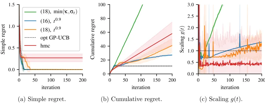
Figure 4: Mean and standard deviation of the empirical simple and cumulative regret over ten different random initializations for the function in Fig. 2. The HMC baseline (red) gets stuck in a local optimum and obtains constant regret in Fig. 4a. GP-UCB with the true
hyperparameters (gray dashed) obtains the lowest cumulative regret in Fig. 4b. However, our methods (orange/blue) increase the function class over time, see Fig. 4c, and thus obtain sublinear regret without knowing the true hyperparameters.
marginalizes them out. Unless otherwise specified, the initial lengthscales are set toθ0 =1, the initial norm bound is B0 = 2, the confidence bounds hold with probability at leastδ= 0.9, and the tradeoff factor betweenb(t) andg(t) isλ= 0.1.
We follow several best-practices in BO to ensure a fair comparison with the baselines. We rescale the input space D to the unit hypercube in order to ensure that both the initial lengthscales and the prior over lengthscales are reasonable for different problems. As is common in practice, the comparison baselines use the empirical confidence intervals suggested in Sec. 4.2, instead of the theoretical bounds in Lemma 1 that are used for our method. Lastly, we initialize all GPs with 2dmeasurements that are collected uniformly at
random within the domainD. To measure performance, we use the cumulative regret that has been the main focus of this paper. In addition, we evaluate the different methods in terms of simple regret, which is the regret of the best inputs evaluated so far, maxx∈Df(x)− maxt0<=tf(xt0). This metric is relevant when costs during experiments do not matter and BO is only used to determine high-quality inputs by the end of the optimization procedure.
5.1. Synthetic Experiments
Example function We first evaluate all proposed methods on the example function in Fig. 2, which lives inside the RKHS associated with a Gaussian kernel with θ = 0.1 and has norm kfkkθ = 2. We evaluate our proposed method for the sublinear reference
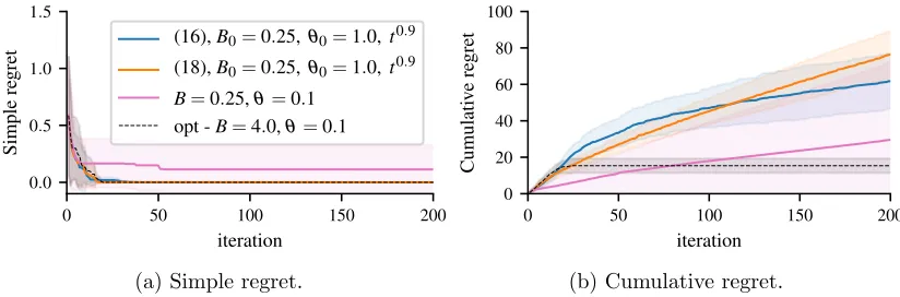
function p(t) = t0.9 together with maximum a posteriori hyperparameter estimation. We compare against bothGP-UCB with the fixed, correct hyperparameters and HMC
ren-0 50 100 150 200 iteration
0.0 0.5 1.0 1.5
Simple
re
gret
(16),B0=0.25, θ0=1.0, t0.9
(18),B0=0.25, θ0=1.0, t0.9 B=0.25,θ=0.1
opt -B=4.0,θ=0.1
(a) Simple regret.
0 50 100 150 200
iteration 0
20 40 60 80 100
Cumulati
ve
re
gret
(b) Cumulative regret.
Figure 5: Simple and cumulative regret over 10 random seeds for samples from a GP with bounded RKHS norm. The GP-UCB algorithm with misspecified hyperparameters
(magenta) fails to converge given only a wrong choice of B0. In contrast, our methods (blue/orange) converge even thoughθ0 is misspecified in addition.
ders σt(xt+1)≥κ= 0.1. This is the most conservative variant of the algorithm. Note that
we do not know a lower bound on the hyperparameters and therefore do not enforce it.
The results of the experiments are shown in Fig. 4. The simple regret plot in Fig. 4a shows that all methods based on hyperparameter adaptation evaluate close-to-optimal in-puts eventually, and do so almost as quickly asGP-UCBbased on the true hyperparameters
(black, dashed). However, the method based on HMC hyperparameter estimation (red) con-siders functions that are too smooth and gets stuck in local optima, as in Fig. 2. This can also be seen in Fig. 4c, which plots the effective scaling g(t) based on the combination of Bayesian hyperparameter estimation and hyperparameter adaptation through h(t). The HMC hyperparameters consistenly over-estimate the lengthscales by a factor of roughly two. In contrast, while the MAP estimation leads to the wrong hyperparameters initially, the adaptation methods in (15) and (16) slowly increase the function class until the true lengthscales are found eventually. It can be seen that the one step estimate (16) (orange) is more noisy than the upper bound in (15) (blue).
0 100 200 300 400 500 iteration
0.00 0.05 0.10 0.15 0.20
Simple
re
gret
(18), min(κ,σt)
(16), t0.9
(18), t0.9
map
(a) Simple regret.
0 100 200 300 400 500
iteration 0
20 40 60 80
Cumulati
ve
re
gret
(b) Cumulative regret.
Figure 6: Simple and cumulative regret over 5 random seeds for a logistic regression problem. All methods determine close-to-optimal parameters. However, our methods explore more to counteract misspecified hyperparameters.
Samples from a GP As a second experiment, we compare GP-UCB to A-GP-UCB
on samples drawn from a GP when the norm bound B0 is misspecified. Samples from a GP are not contained in the RKHS. To avoid this technical issue, we sample function values from the posterior GP at only a finite number of discrete gridpoints and interpolate between them using the kernel with the correct lengthscales θ. We rescale these functions to have RKHS norm ofB = 4, but useB0= 0.25 as an initial guess for both BO algorithms and do not use any hyperparameter estimation. Even though we use the correct kernel lengthscales for GP-UCB, θ0 = θ = 0.1, this discrepancy means that the true function is not contained in the initial confidence intervals. As before, for our method we use the reference regretp(t) =t0.9 and additionally misspecify the lengthscales,θ
0= 1.
The results are shown in Fig. 5. GP-UCB with the correct hyperparameters (black,
dashed) obtains the lowest cumulative regret. However, it fails to converge when hyperpa-rameters are misspecified (magenta), since the confidence intervals are too small to encour-age any exploration. In contrast, our methods (blue/orange) converge to close-to-optimal inputs as in the previous example.
5.2. Logistic Regression Experiment
Lastly, we use our method to tune a logistic regression problem on the MNIST data set (Le-Cun, 1998). As in the experiment in Klein et al. (2016), we consider four training inputs: the learning rate, the l2 regularization constant, the batch size, and the dropout rate. We use the validation loss as the optimization objective.
The results are shown in Fig. 6. Even though the input space is fairly high-dimensional with d= 4, all algorithms determine close-to-optimal inputs quickly. In particular, MAP estimation determines that both the dropout rate and the batch size do not influence the validation loss significantly. Since the theoretical results inA-GP-UCBare compatible with
to be more confident that the global optimum has been identified astincreases. For standard BO methods, there is no guarantee of convergence with misspecified hyperparameters.
6. Conclusion and Future Work
We introduced A-GP-UCB, a BO algorithm that is provably no-regret when
hyperpa-rameters are unknown. Our method adapts the hyperpahyperpa-rameters online, which causes the underlying BO algorithm to consider larger function spaces over time. Eventually, the function space is large enough to contain the true function, so that our algorithm provably converges. We evaluated our method on several benchmark problems, confirming that, on the one hand, it provably converges even in cases where standard BO algorithms get stuck in local optima, and, on the other hand, enjoys competitive performance as standard BO algorithms that do not have theoretical guarantees in this setting.
The main idea behind our analysis is that adapting the hyperparameters increases the cumulative regret bound, but we do so slowly enough to converge eventually. This idea is fairly general and could also be applied to other no-regret algorithms. Another poten-tial future direction is to investigate alternative strategies to select the scaling factorsb(t) and g(t) and consider adapting other parameters such as the kernel structure.
Acknowledgments
This research was supported in part by SNSF grant 200020 159557, ERC grant no. 815943, NSERC grant RGPIN-2014-04634, the Vector Institute, and an Open Philantropy Project AI fellowship. We would like to thank Johannes Kirschner for valueable discussions.
References
Yasin Abbasi-Yadkori. Online learning of linearly parameterized control problems. PhD thesis, 2012.
Hany Abdelrahman, Felix Berkenkamp, and Andreas Krause. Bayesian optimization for maximum power point tracking in photovoltaic power plants. In 2016 European Control Conference (ECC), pages 2078–2083, 2016.
James Bergstra and Yoshua Bengio. Random search for hyper-parameter optimization.
Journal of Machine Learning Research, 13(Feb):281–305, 2012.
Felix Berkenkamp, Andreas Krause, and Angela P. Schoellig. Bayesian optimization with safety constraints: safe and automatic parameter tuning in robotics. arXiv:1602.04450 [cs.RO], 2016.
Ilija Bogunovic, Jonathan Scarlett, Andreas Krause, and Volkan Cevher. Truncated vari-ance reduction: a unified approach to Bayesian optimization and level-set estimation. In
Eric Brochu, Vlad M. Cora, and Nando de Freitas. A tutorial on Bayesian optimization of expensive cost functions, with application to active user modeling and hierarchical reinforcement learning. arXiv:1012.2599 [cs], 2010.
Adam D. Bull. Convergence rates of efficient global optimization algorithms. Journal of Machine Learning Research, 12(Oct):2879–2904, 2011.
Roberto Calandra, Andr´e Seyfarth, Jan Peters, and Marc Peter Deisenroth. An exper-imental comparison of Bayesian optimization for bipedal locomotion. In 2014 IEEE International Conference on Robotics and Automation (ICRA), pages 1951–1958, 2014.
Sayak Ray Chowdhury and Aditya Gopalan. On kernelized multi-armed bandits. In Proceed-ings of the 34th International Conference on Machine Learning, volume 70 ofProceedings of Machine Learning Research, pages 844–853. PMLR, 2017.
Andreas Christmann and Ingo Steinwart. Support Vector Machines. Information Science and Statistics. Springer, New York, NY, 2008.
Josip Djolonga, Andreas Krause, and Volkan Cevher. High-dimensional Gaussian process bandits. In Advances in Neural Information Processing Systems 26, pages 1025–1033, 2013.
Audrey Durand, Odalric-Ambrym Maillard, and Joelle Pineau. Streaming kernel regression with provably adaptive mean, variance, and regularization. Journal of Machine Learning Research, 19(17):1–34, 2018.
David K. Duvenaud, Hannes Nickisch, and Carl Edward Rasmussen. Additive Gaussian processes. In Advances in Neural Information Processing Systems 24, pages 226–234, 2011.
Peter Frazier, Warren Powell, and Savas Dayanik. The knowledge-gradient policy for cor-related normal beliefs. INFORMS Journal on Computing, 21(4):599–613, 2009.
Daniel Golovin, Benjamin Solnik, Subhodeep Moitra, Greg Kochanski, John Karro, and D. Sculley. Google vizier: a service for black-box optimization. InProc. of the 23rd ACM SIGKDD International Conference on Knowledge Discovery and Data Mining, KDD ’17, pages 1487–1495, New York, NY, USA, 2017. ACM.
I. S. Gradshte˘ın, I. M. Ryzhik, and Alan Jeffrey. Table of integrals, series, and products. Academic Press, Amsterdam, Boston, 7th ed edition, 2007.
Philipp Hennig and Christian J. Schuler. Entropy search for information-efficient global optimization. Journal of Machine Learning Research, 13(1):1809–1837, 2012.
Motonobu Kanagawa, Philipp Hennig, Dino Sejdinovic, and Bharath K. Sriperumbudur. Gaussian processes and kernel methods: a review on connections and equivalences.
arXiv:1807.02582 [stat.ML], 2018.
Johannes Kirschner and Andreas Krause. Information directed sampling and bandits with heteroscedastic noise. In Proceedings of the 31st Conference On Learning Theory, vol-ume 75 of Proceedings of Machine Learning Research, pages 358–384. PMLR, 2018.
Aaron Klein, Stefan Falkner, Jost Tobias Springenberg, and Frank Hutter. Bayesian neural network for predicting learning curves. InNIPS 2016 Bayesian Neural Network Workshop, 2016.
Yann LeCun. The mnist database of handwritten digits.
http://yann.lecun.com/exdb/mnist/, 1998.
Daniel J. Lizotte, Tao Wang, Michael H. Bowling, and Dale Schuurmans. Automatic gait optimization with Gaussian process regression. In Proceedings of the Twentieth Inter-national Joint Conference on Artificial Intelligence (IJCAI), volume 7, pages 944–949, 2007.
Jonas Mockus. Bayesian approach to global optimization: theory and applications. Springer Science & Business Media, 2012.
Jonas Mockus, Vytautas Tiesis, and Antanas Zilinskas. The application of Bayesian methods for seeking the extremum. Towards Global Optimization, 2:117–129, 1978.
Carl Edward Rasmussen and Christopher K.I Williams. Gaussian processes for machine learning. MIT Press, Cambridge MA, 2006.
Binxin Ru, Michael A. Osborne, Mark Mcleod, and Diego Granziol. Fast information-theoretic Bayesian optimisation. In Proceedings of the 35th International Conference on Machine Learning, volume 80 of Proceedings of Machine Learning Research, pages 4384–4392. PMLR, 2018.
Daniel Russo and Benjamin Van Roy. Learning to optimize via information-directed sam-pling. In Z. Ghahramani, M. Welling, C. Cortes, N. D. Lawrence, and K. Q. Weinberger, editors,Advances in Neural Information Processing Systems 27, pages 1583–1591. Curran Associates, Inc., 2014.
M. W. Seeger, S. M. Kakade, and D. P. Foster. Information consistency of nonparametric Gaussian process methods. IEEE Transactions on Information Theory, 54(5):2376–2382, 2008.
Jasper Snoek, Kevin Swersky, Richard S. Zemel, and Ryan P. Adams. Input warping for Bayesian optimization of non-stationary functions. In NIPS Workshop on Bayesian Optimization, 2013.
Niranjan Srinivas, Andreas Krause, Sham M. Kakade, and Matthias Seeger. Gaussian process optimization in the bandit setting: no regret and experimental design. IEEE Transactions on Information Theory, 58(5):3250–3265, 2012.
V. Vapnik. Principles of risk minimization for learning theory. In J. E. Moody, S. J. Hanson, and R. P. Lippmann, editors,Advances in Neural Information Processing Systems 4, pages 831–838. Morgan-Kaufmann, 1992.
Kim Peter Wabersich and Marc Toussaint. Advancing Bayesian optimization: the mixed-global-local (mgl) kernel and length-scale cool down. arXiv:1612.03117 [cs, stat], 2016.
Zi Wang and Stefanie Jegelka. Max-value entropy search for efficient Bayesian optimization. In Proceedings of the 34th International Conference on Machine Learning, volume 70 of
Proceedings of Machine Learning Research, pages 3627–3635. PMLR, 2017.
Ziyu Wang and Nando de Freitas. Theoretical analysis of Bayesian optimisation with un-known Gaussian process hyper-parameters. arXiv:1406.7758 [cs, stat], 2014.
Ziyu Wang, Frank Hutter, Masrour Zoghi, David Matheson, and Nando de Freitas. Bayesian optimization in a billion dimensions via random embeddings. Journal of Artificial Intel-ligence Research, 55:361–387, 2016.
Appendix A. Proof of Main Theorem
Lemma 3 Let f ∈ Hθt∗ with kfkθt∗ ≤Bt∗. Then, for any monotonically increasing
func-tions g(t)≥1 and b(t)≥1 and for all t≥t∗: f ∈ H
θt with kfkθt ≤Bt
Proof Lemma 2 together with monotonicity of gyieldsHθt ⊇ Hθt∗ so that f ∈ Hθt and
kfkθt ≤
Y
1≤i≤d
[θt∗]i [θt]i k
fkθt∗ ≤
g(t)d
g(t∗)dBt∗=
g(t)d
g(t∗)dg(t
∗)db(t∗)B
0 =g(t)db(t∗)B0≤Bt
Lemma 4 Under the assumptions of Lemma 1, let θt be a predictable sequence of kernel
hyperparameters such that kfkkθt ≤Bt and let the GP predictions µt and σt use the prior
covariancekθt. Ifβt1/2 =Bt+ 4σ
p
Iθt(yt;f) + 1 + ln(1/δ), then|f(x)−µt(x)| ≤βt1/2σt(x)
holds for allx∈D and iterations t≥0 jointly with probability at least 1−δ.
We are now ready to prove the main result:
Proof [Theorem 1] We split the regret bound into two terms,Rt=t0rc+rs(t). In the
ini-tial rounds, where either Bt≤g(t)dB0 or maxi[θ]i/[θ]0>1, the regret is trivially bounded by rt ≤ 2kfk∞ ≤ 2kfkθ ≤ B. Thus rc ≤ 2B. Let t0 ∈ (0,∞] be the first iteration such that f ∈ Hθt0 with kfkθt0 ≤ Bt0. From Lemma 3, we have thatf ∈ Hθt with kfkθt ≤Bt
for all t≥t0. Thus we can use Lemma 4 to conclude |f−µt(x)| ≤βt1/2σt(x) for all x∈ D
andt≥t0 jointly with probability at least (1−δ). We use Lemmas 5.2-5.4 in Srinivas et al. (2012) to conclude that the second stage has a regret bound ofr2
s(t)≤C1βtI(yt;f), which
concludes the proof.
Appendix B. Bound on the information capacity γt
Theorem 4 (Theorem 8 in Srinivas et al. (2012)) Suppose that D⊂Rd is compact, and k(x,x0) is a covariance function for which the additional assumption of Theorem 2 in Srinivas et al. (2012) hold. Moreover, let Bk(T∗) =Ps>T∗λs, where {λs} is the
op-erator spectrum of k with respect to the uniform distribution over D. Pick τ > 0, and let nT =C4Tτ(logT) with C4 = 2V(D)(2τ + 1). Then, the following bound holds true:
γT ≤
1/2
1−e−1 r∈{1max,...,T}T∗log
rnT
σ2
+C4σ−2(1−
r
T)(Bk(T∗)T
τ+1+ 1) logT +O(T1−τ d).
(19)
Theorem 4 allows us to bound γt through the operator spectrum of the kernel with
respect to the uniform distribution. We now consider this quantity for two specific kernels.
B.1. Bounds for the Squared Exponential Kernel
Lemma 5 For all x∈[0, x2
max] it holds thatlog(1 +x2)≥
log(1+x2
max)
x2
max x
2
In this section, we use Theorem 4 to obtain concrete bounds for the Gaussian kernel. From Seeger et al. (2008), we obtain a bound on the eigenspectrum that is given by
λs≤cBs
1/d
, wherec=
r
2a
A, b=
1 2θ2
t
, B = b
A, and A=a+b+
p
a2+ 2ab.
The constanta >0 parameterizes the distributionµ(x)∼ N(0,(4a)−1I
d). As a consequence
ofθt>0, we have that b≥0, 0< B <1,c >0, and A >0. In the following, we bound the
eigenspectrum. The steps follow the outline of Seeger et al. (2008), but we provide more details and the dependence on the lengtscales θt is made explicit:
Bk(T∗) =
X
s>T∗
λs≤c
X
s≥T∗+1
Bs1/d =c X
s≥T∗+1
exp log(Bs1/d) =c X
s≥T∗+1
exp(s1/dlogB),
=c X
s≥T∗+1
exp(−s1/dα)≤c
Z ∞
T∗
where α=−logB. Now substitutes=φ(t) = (t/α)d. Then ds= dtd−1
α dtand
Bk(T∗)≤c
Z ∞
αT∗1/d
exp(−t)dt
d−1
α dt=cdα
−dΓ(d, αT1/d
∗ ),
where Γ(d, β) =R∞
β e
−ttd−1dt= (d−1)!e−βPd−1
k=0βk/k! for d∈Nas in Gradshte˘ın et al. (2007, (8.352.4)). Then, with β=αT∗1/d,
Bk(T∗)≤cdα−d(d−1)!e−β
d−1
X
k=0
βk/k! =c(d!)α−de−β
d−1
X
k=0
(k!)−1βk.
Before we bound the information gain, let us determine how α−d and c depend on the
lengthscales. In particular, we want to quantify their upper bounds in terms ofg(t).
α−d= log−d(1/B) = log−d 2θ2
tA
= log−d
1 + 2θ2
ta+ 2θt
r
a2+ a
θ2
t
(20)
≤log−d 1 + 2θ2ta
≤
log(1 + 2θ2 0a) 2θ2
0a
2θ2ta
−d
by Lemma 5 (21)
=Oθ−2t d=Og2d(t), (22) where (21) follows from Lemma 5, since g(t)≥1 for allt >0. Similarly,
c=
2a
a+ 21θ2
t +
q
a2+ a
θ2t
d/2
≤ 21a 2θ2t
!
= 4aθ2
t
d/2
=O(g(t)−d). (23)
As in Srinivas et al. (2012), we choose T∗ = (log(T nT)/α)d, so that β = log(T nT) and
therefore does not depend ongt. Plugging into (19), the first term of (19) dominates and
γT =O
h
log(Td+1(logT))id+1cα−d
d/2
=O(logT)d+1g(t)d. (24)
B.2. Mat´ern kernel
Following the proof for Theorem 2 in the addendum to Seeger et al. (2008), we have that
λ(sT)≤C(1 +δ)s−(2ν+d)/d ∀s≥s0, (25)
For the leading constant we have C = C3(2ν+d)/d with α = 2√πθt
2ν. Hiding terms that do
not depend on α and thereforeg(t), we have
Ct(α, ν) =
Γ(ν+d/2)
πd/2Γ(ν) α
d=O(g(t)−d) c
1 =
1 (2π)dC
t(α, ν)
=O(g(t)d)
C2=
α−d
2dπd/2Γ(d/2) =O(g(t)
d) C
3 =C2 2 ˜C
d c
−d 2ν+d
1 =O(g(t)
dg(t)2−νd+2d) =
O(g(t)d),
so that C = O(g(t)2ν+d). The second term in C
3 must be over-approximated as a con-sequence of the proof strategy. It follows that Bk(T∗) = O(g(t)2νdT∗1−(2ν+d)/d) and, as in Srinivas et al. (2012), thatγT =O(T
d(d+1)