Semi-Analytic Resampling in Lasso
Tomoyuki Obuchi [email protected]
Yoshiyuki Kabashima [email protected]
Department of Mathematical and Computing Science Tokyo Institute of Technology
2-12-1, Ookayama, Meguro-ku, Tokyo, Japan
Editor:Jon McAuliffe
Abstract
An approximate method for conducting resampling in Lasso, the `1 penalized linear re-gression, in a semi-analytic manner is developed, whereby the average over the resampled datasets is directly computed without repeated numerical sampling, thus enabling an in-ference free of the statistical fluctuations due to sampling finiteness, as well as a significant reduction of computational time. The proposed method is based on a message passing type algorithm, and its fast convergence is guaranteed by the state evolution analysis, when covariates are provided as zero-mean independently and identically distributed Gaussian random variables. It is employed to implement bootstrapped Lasso (Bolasso) and stability selection, both of which are variable selection methods using resampling in conjunction with Lasso, and resolves their disadvantage regarding computational cost. To examine approximation accuracy and efficiency, numerical experiments were carried out using simu-lated datasets. Moreover, an application to a real-world dataset, the wine quality dataset, is presented. To process such real-world datasets, an objective criterion for determining the relevance of selected variables is also introduced by the addition of noise variables and re-sampling. MATLAB codes implementing the proposed method are distributed in (Obuchi, 2018).
Keywords: bootstrap method, Lasso, variable selection, message passing algorithm, replica method
1. Introduction
Variable selection is an important problem in statistics, signal processing, and machine learning. A desire for useful techniques of variable selection has recently been growing, as cumulated advances in measurement and information technologies have started to steadily produce a large amount of high-dimensional data in science and engineering. A naive method for selecting relevant variables requires solving discrete optimization problems. This involves a serious computational difficulty as the dimensionality of the variables increases, even in the simplest case of linear models (Natarajan, 1995). Hence, certain relaxations or approximations are required for handling such large high-dimensional datasets.
A great deal of progress has been made with regard to relaxation techniques by intro-ducing an`1 penalty (Tibshirani, 1996; Meinshausen and B¨uhlmann, 2004; Banerjee et al., 2006; Friedman et al., 2008). Its model consistency, that is, whether the estimated model
c
converges to the true model in the large size limit of data, has been extensively studied, particularly in the case of linear models (Knight and Fu, 2000; Zhao and Yu, 2006; Yuan and Lin, 2007; Wainwright, 2009; Meinshausen and Yu, 2009). These studies show that a naive usage of the `1 penalty affects model consistency in realistic settings: The resultant estimator cannot completely reject variables not present in the true model if there exist non-trivial correlations between covariates, although the normal consistency in the`2 sense is retained. This fact motivated the development of further techniques for recovering model consistency in the variable selection context, particularly in the last decade, including tradi-tional approaches using confidence interval and hypothesis testing (Zou, 2006; Bach, 2008; Meinshausen and B¨uhlmann, 2010; Javanmard and Montanari, 2014a,b, 2015; Lockhart et al., 2014; G’Sell et al., 2013; Takahashi and Kabashima, 2018). If the distribution of the estimator is accurately figured out and the corresponding P-value is efficiently computed, those traditional approaches are quite efficient and powerful enough to correctly perform variable selection. However in many practical situations, the functional form of the distribu-tion is not clear. In such cases, certain numerical approaches are employed to approximately estimate the distribution. Resampling is one of the representative methods and is focused on in the present paper.
Resampling is a versatile idea applicable to a wide range of problems in statistical mod-eling and is broadly used in machine learning algorithms; some examples can be found in boosting and bagging (Trevor et al., 2009). In statistics, Efron’s bootstrap method is a pioneering example in which resampling is efficiently and systematically used (Efron and Tibshirani, 1994). In the case of the `1-penalized linear regression or Lasso (Tibshirani, 1996), through a fine evaluation of each variable’s probability to be selected (positive prob-ability) in a fairly general setting, Bach showed that it is possible to perform statistically consistent variable selection by utilizing the bootstrap method (Bach, 2008); the associated algorithm is called bootstrapped Lasso (Bolasso). Another algorithm based on a similar idea, calledstability selection(SS), was also implemented by randomizing the penalty coef-ficient in Lasso (Meinshausen and B¨uhlmann, 2010). All these examples demonstrate that resampling is powerful and versatile.
A common disadvantage of such resampling approaches is their computational cost. For example, in the Bolasso case, the`1-penalized linear regression should be recursively solved according to the number of resampled datasets, which should be sufficiently large so that the positive probability of variables may be estimated. This multiple computational cost precludes the application of such resampling techniques to large datasets. The aim of this study is to avoid this problem by developing an approximation whereby the resampling is conducted in a semi-analytic manner, and to implement it in Lasso.
Such an approximation was already obtained by Malzahn and Opper (2003), where a general framework of semi-analytic resampling was developed using the replica method from statistical mechanics, and was demonstrated in Gaussian process regression. We follow their idea and pursue how it works in Lasso with certain resampling manners.
be adopted. In this study, Gaussian approximation is used in conjunction with the so-called cavity method, providing a message passing type algorithm. Its dynamical behavior is analyzed by the so-called state evolution, which guarantees that the algorithm convergence is free from the model dimensionality and the dataset size when covariates are provided as zero-mean independently and identically distributed (i.i.d.) Gaussian random variables. They are explained in Section 3. In Section 4, numerical experiments are carried out on both simulated and real-world datasets to examine the accuracy and efficiency of the proposed semi-analytic method. For processing real-world datasets, an objective criterion for determining the relevance of selected variables is also proposed, based on the addition of noise variables and resampling. The last section concludes the paper.
2. Formulation for semi-analytic resampling
Let us start from preparing notations and definitions. We denote by D a given dataset, which usually consists of a set of inputs xµ and outputs yµ as D = {(xµ, yµ)}Mµ=1, and denote our basic statistics by ˆβ(D) = ( ˆβ1(D),· · · ,βˆN(D))>. They are interpreted as an
estimator of true parameters in the true model that is inferred. Based on the Bayesian inference framework, it is assumed that the basic estimator can be expressed as an average over a certain posterior distributionP(β|λ, D), that is,
ˆ
β(λ, D) =
Z
dβ βP(β|λ, D)≡ hβi, (1)
where h·i represents the average over the posterior distribution which is supposed to be constructed as follows:
P(β|λ, D) = 1
Z(λ, D)P0(β|λ)P(D|β). (2) Here, P0(β|λ) is the prior distribution characterized by the parameters λ, and P(D|β) represents the likelihood. The normalization constant or the partition function can be explicitly expressed by
Z(λ, D) =
Z
dβP0(β|λ)P(D|β). (3) Considering the construction of a subsample by resampling from the full data Dof size
M with replacement, let an indicator vector c= (c1,· · ·, cM)> specify any such subsample;
each cµis a non-negative integer counting the number of occurrences of theµ-th datapoint
of D in the subsample. A subsample identified by c is denoted by Dc. Specifying a
resampling defines the distribution P(c) ofc, and the question is the behavior of the basic estimators and their functions with respect to the average over P(c). In some resampling techniques, additional randomization is introduced in the prior distribution (Meinshausen and B¨uhlmann, 2010). Hence, an average over the parameters λ is further considered, and the distribution P(λ) of λ is introduced. For notational simplicity, the average over these distributions is denoted by square brackets with appropriate subscripts as follows:
[(· · ·)]c,λ≡X
c
Z
dλ(· · ·)P(c)P(λ).
2.1. General theory of semi-analytic resampling
The purpose of resampling is to obtain the distribution of the basic estimator
P(βi) =
h
δβi−βˆi(λ, Dc)
i
c,λ, (4)
which is reduced to computing the momentshβˆir(λ, Dc)
i
c,λof arbitrary degree
∀r∈N. We
thus show that these moments can be evaluated in the following manner. By definition, the moment
h
ˆ
βir(λ, Dc)
i
c,λ withr∈Ncan be written as
h
ˆ
βir(λ, Dc)
i
c,λ=
"
1
Zr(λ, D c)
Z ( r
Y
a=1
dβaβiaP0(βa|λ)P(Dc|βa)
)#
c,λ
(5)
= lim
n→0
"
Zn−r(λ, Dc)
Z ( r
Y
a=1
dβaβiaP0(βa|λ)P(Dc|βa)
)#
c,λ
(6)
.
= lim
n→0
"
Z ( n
Y
b=1
dβb
) ( r
Y
a=1
βia
) ( n
Y
b=1
P0(βb|λ)P(Dc|βb)
)#
c,λ
. (7)
The evaluation of (5) is technically difficult owing to the existence of Zr(λ, Dc) in the
denominator: The negative power of the partition function does not allow the analytical evaluation of the average over c and λ, even if P(c) and P(λ) take reasonable forms. To overcome this difficulty, an auxiliary parameter n is introduced in (6). The exponent n is assumed to be a positive integer larger thanrin (7); thus, the power of the partition function can be expanded in the integral form (3). Integral variables {β1,β2, . . . ,βn} are termed replicas since they are regarded as constitutingn copies of the original system. In (7), the configurational average can be analytically computed under appropriate approximations. This yields an expression as a function of n that is analytically continuable from N to R. The n→ 0 limit is taken by employing the analytically continued expression after all
computations. The evaluation technique based on these procedures is often called thereplica method(M´ezard et al., 1987; Nishimori, 2001; Dotsenko, 2005). Evidently, this technique is not justified in a strict sense, but it is known that the replica method gives correct results for many problems. Justification of the replica method is known to be difficult (Talagrand, 2003), and here we leave it as a future work and just employ the method for our purpose. In the present problem, it is far from trivial to obtain an analytically continuable expression, and below we concentrate on its derivation.
Accordingly, the configurational average of any power of the basic estimator can be evaluated from the following quantities:
Ξ ({βa}na=1|D)≡
Z ( n
Y
a=1
dβa
) " n Y
a=1
P0(βa|λ)P(Dc|βa)
#
c,λ
,
P({βa}na=1|D)≡ 1 Ξ ({βa}n
a=1 |D)
" n Y
a=1
P0(βa|λ)P(Dc|βa)
#
c,λ
where the former is called replicated partition function and the latter is called replicated Boltzmann distribution. The average over the replicated Boltzmann distribution is denoted by
(· · ·)≡
Z ( n
Y
a=1
dβa
)
(· · ·)P({βa}na=1 |D). (8)
It follows from (5)–(7) that this average converges to the desired total average over the posterior and the configurational variablesc and λasn→0. The next step is to compute this average. The nontrivial technical difficulties are in the integrations with respect to replicas {βa}n
a=1 and in deriving a functional form that is analytically continuable with respect ton. These will be handled after considering the specific case of Lasso.
2.2. Specifics to Lasso with independent sampling
The above general theory is now rephrased in the context of Lasso. Given a set of covariates
xµ∈RN and responsesyµ∈R,D={(xµ, yµ)}Mµ=1, the usual estimator by Lasso is
ˆ
β(λ, D) = arg min
β
1 2
M
X
µ=1
yµ−
X
i
xµiβi
!2
+λ||β||1
.
In contrast to this, considering Bolasso and SS, given the resampled data Dc and the
randomized penalty coefficients λ= (λ1,· · ·, λN)>, the following estimator is introduced:
ˆ
β(λ, Dc) = arg min β
1 2
M
X
µ=1
cµ yµ−
X
i
xµiβi
!2
+
N
X
i=1
λi|βi|
. (9)
For representing this in terms of the posterior average, the following quantities are intro-duced:
H(β|λ, Dc) =
1 2
M
X
µ=1
cµ yµ−
X
i
xµiβi
!2
+
N
X
i=1
λi|βi|,
Zγ(λ, Dc) =
Z
dβe−γH(β|λ,Dc), Pγ(β|λ, Dc) =
1
Zγ
e−γH(β|λ,Dc),
where these quantities are called (in the order they appear) Hamiltonian, partition func-tion, and Boltzmann distribufunc-tion, in accordance with physics terminology. As γ → ∞, the Boltzmann distribution converges to a pointwise measure at ˆβ(λ, Dc) and thereby becomes
the desired posterior distribution, allowing the identification of the Boltzmann distribution with the posterior distribution; thus, the average over the Boltzmann distribution is there-after denoted byh· · ·iintroduced in (1)1. The prior distributionP0(β|λ) and the likelihood
P(D|β) in (2) correspond to the factors e−γP
iλi|βi| and e−γ2
PM
µ=1cµ(yµ−Pixµiβi)
2
in the Boltzmann distribution, respectively.
Considering Bolasso and SS, we draw the subsample c of a fixed size m in an unbiased manner. Each sample comes out with a probability of M−mm!/(c
1!· · ·cM!), which has a
weak dependency among{cµ}µ. However, this dependency is not essential for largeM and
m; thus, it is ignored. Using Stirling’s formula m!≈(me)m in conjunction with the relation
m=PM
µ=1cµ,cµis approximately regarded as an i.i.d. variable from a Poisson distribution of meanτ =m/M, namely,
P(c) =
M
Y
µ=1
τcµ cµ!
e−τ =
M
Y
µ=1
P(cµ).
It is also natural to require thatP(λ) is factorized into a batch of identical distributions as follows:
P(λ) =
N
Y
i=1
P(λi).
At this point, the explicit form ofP(λi) is not specified. These factorized natures allow us
to express the replicated Boltzmann distribution as
Pγ({βa}na=1|D)∝
h
e−γPna=1H(βa|λ,Dc)
i
c,λ=
M
Y
µ=1
Φµ {βi}Ni=1
N
Y
i=1
Ψ (βi), (10)
where
Φµ {βi}Ni=1
=he−12γc P
a(yµ−Pixµiβia)
2i
c,
Ψ (βi) =
h
e−γλPna=1|βia| i
λ,
and the vector notation βi = (βia)a was introduced for later convenience. Φµ is hereafter
calledµ-th potential function.
To proceed further, an approximation should be introduced to make the right-hand side of (10) tractable. Although there are several ways for that, we here make an approximation based on the cavity method from statistical physics. The details are in the next section.
3. Handling the replicated system
(10) implies that the replicated Boltzmann distribution naturally has a factor graph structure. Hence, by the cavity method, (10) can be “approximately” decomposed into two messages as follows:
e
φµ→i(βi) =
1
Zµ→i
Z Y
j(6=i)
dβj Φµ {βi}Ni=1
Y
j(6=i)
φj→µ(βj), (11)
φi→µ(βi) =
1
Zi→µ
Ψ (βi)
Y
ν(6=µ)
e
φν→i(βi), (12)
where Zµ→i, Zi→µ are normalization factors that are not relevant and will be discarded
below. The average of (8) can be computed by employing this set of equations.
3.1. Gaussian approximation on cavity method
A crucial observation for assessing (11),(12) is that the residual Raµ = yµ−Pjxµjβja
ap-pearing in Φµ has a sum of a large number of random variables; thus, the central limit
theorem justifies treating it as a Gaussian variable with the appropriate mean and variance. This consideration leads to the following decomposition in (11)
Rµa+xµiβia≡yµ−
X
j(6=i)
xµjβja≈yµ−
X
j(6=i)
xµjβ
\µ
j +Zµia ≡rµi+Zµia,
where Zµia is a zero-mean Gaussian variable whose covariance is equivalent to that of
P
j(6=i)xµjβja, and (· · ·)
\µ
is the average over Q
jφj→µ(βj) or the replicated Boltzmann
distribution without µ-th potential function. This shows that it is difficult to consider the correlation between βi and βj with different i, j in the present framework. This could be
overcome even in the cavity method framework (Opper and Winther, 2001a,b); however, it is beyond the scope of this study.
The so-called replica symmetry is now assumed in the messages. This symmetry implies that any permutation of the replicas {β1i,· · ·, βin} yields an identical message, which in turn implies, by De Finetti’s theorem (Hewitt and Savage, 1955), that the messages can be expressed as
φi→µ(βi) =
Z
dFρi→µ(F) n
Y
a=1
F(βia),
e
φµ→i(βi) =
Z
dGρµ→i(G) n
Y
a=1
wheredFρi→µ(F) anddGρi→µ(G) are probability measures over the probability distribution
functionsF andG, respectively. From this form, two different variances naturally emerge:
Vi\µ≡(βia)2−βiaβib
\µ
=
Z dβi
(βia)2−βiaβib Z
dFρi→µ(F) n
Y
c=1
F(βci)
=
Z
dFρi→µ(F)
( Z
F(β)β2dβ− Z
F(β)βdβ 2)
,
Wi\µ≡βa iβib
\µ
−βa i \µ βb i \µ = Z
dFρi→µ(F)
Z
F(β)βdβ 2
− Z
dFρi→µ(F)
Z
F(β)βdβ 2
,
where it was assumed that a6=b. Below, theµ-dependence of Vi\µ and Wi\µ is ignored, as it is small, and let
Vi\µ≈Vi= (βia)2−βiaβib,
Wi\µ≈Wi =βiaβib−βiaβib.
It can be implied that Vi describes the average of the variance inside a fixed resampled
dataset, whereas Wi represents the inter-sample variance. UsingVi and Wi, the covariance
of βi is generally written as
Cov\µβia, βbi≡βa iβib
\µ
−βa i
\µ
βb i
\µ
=Wi\µ+Vi\µδab≈Wi+Viδab.
Using this relation, the covariance of{Zµia}a can be expressed as
Cov\µZµia, Zµib = X
j,k(6=i)
xµixµjCov\µ
βja, βkb≈X
j
x2µjCov\µβja, βjb
≈X
j
x2µj(Wj+Vjδab)≡Wµ+Vµδab.
The correlation between βj and βk for j 6= k is neglected in the second sum because it
is not taken into account in the present framework, as explained above. Moreover, the addition of the i-th term in the same sum does not affect the following discussion because it is sufficiently small in the summation. Based on these observations, Zµia is decomposed as follows:
Zµia =Dµi+ ∆aµi,
whereDµiand ∆aµiare zero-mean Gaussian variables whose covariances are Cov\µ(Dµi, Dµi) =
Wµ, Cov\µ
Dµi,∆aµi
= 0, Cov\µ∆aµi,∆bµi=Vµδab.
e
φµ→i can now be computed. The integration with respect to{βj}j(6=i)in (11) is replaced by that overDi and ∆ai. The result is
e
φµ→i(βi)≈
Z
dDµiP(Dµi)
Z Y
a
d∆aµiP(∆aµi)he−12γc P
a(rµi−xµiβia+Dµi+∆aµi)2 i
c
=
h
U(c)−12 (1 +cγVµ)−
n
2 e−
1 2S(c)
P
a(rµi−xµiβai)
2
+12T(c)(P
a(rµi−xµiβia))
2i
where
S(c) = cγ 1 +cγVµ
,
T(c) = c
2γ2W
µ
(1 +cγVµ)(1 +cγ(Vµ+nWµ))
,
U(c) = 1 +cγ(Vµ+nWµ) 1 +cγVµ
.
lnφeµ→i(βi) can be expanded with respect to xµiβia, and the expansion up to the second
order leads to an effective Gaussian approximation of the message, yielding
e
φµ→i(βi)≈e− 1 2γA˜µ→i
P
a(βia)
2
+1 2γ
2C˜µ→i(P
aβai)
2
+γB˜µ→iPaβia,
where
˜
Aµ→i =
c
1 +cγVµ
c
x2µi, (16a)
˜
Bµ→i=
c
1 +cγVµ
c
rµixµi, (16b)
˜
Cµ→i=
("
c
1 +cγVµ
2#
c
Wµ+
"
c
1 +cγVµ
2#
c
−
c
1 +cγVµ
2
c
!
(rµi)2
)
x2µi.(16c) It should be noted that then→0 limit was already taken in these coefficients.
Owing to the Gaussian approximation of φeµ→i(βi), the marginal distribution of the
replicated Boltzmann distribution can be simply written as
Pi(βi|D)≡
Z Y
j(6=i)
dβjP({βi}i|D)∝Ψ(βi)
Y
µ
e
φµ→i(βi)
≈ Z
Dz eγ
−1 2Ai
P
a(βai)
2
+(Bi+
√
Ciz)
P
aβia−λ
P
a|βia|
λ
, (17)
whereDz=dze−12z 2
/√2π, and the following identity was used:
e12Cx 2 = Z Dz e √ Czx.
Moreover, Ai = PµA˜µ→i, Bi = PµB˜µ→i, and Ci = PµC˜µ→i. All replicas are now
factorized, and the average can be taken for each replica independently, allowing passing to then→0 limit by analytic continuation from Nto Rwith respect to n. For example, the
mean ofβai is computed as
βa
i =
Z Dz
Z
dβ eγ(−12Aiβ 2+(B
i+
√
Ciz)βi−λ|β|) n−1
λ × " Z Dz Z
dβ βeγ(−12Aiβ 2+(B
i+
√
Ciz)βi−λ|β|) Z
dβ eγ(−12Aiβ 2+(B
i+
√
Ciz)βi−λ|β|) n−1#
λ n→0 −−−→ " Z Dz R
dβ βeγ(−12Aiβ 2+(B
i+
√
Ciz)βi−λ|β|) R
dβ eγ(−12Aiβ2+(Bi+
√
Ciz)βi−λ|β|) #
λ
γ→∞
−−−→ Z
DzSλ(Bi+
p
Ciz;Ai)
λ
whereSλ is the so-called soft thresholding function
Sλ(x;A) =
1
A(x−λsgn (x))θ(|x| −λ),
andθ(x) is the step function that is equal to 1 ifx >0 and 0 otherwise. Thus, the mean of the basic estimator takes a reasonable form.
In the above average, it is assumed that the coefficientsAi, Bi, Ciremain finite asγ → ∞.
This is the case if the following holds:
χµ≡γVµ=
X
i
x2µiγVi→O(1), (γ → ∞).
This scaling is consistent, which can be shown by
χi ≡γVi =γ
n
(βa
i)
2−βa iβib
o n→0 −−−→ Z Dz γ R
dβ β2eγ(−12Aiβ 2+(B
i+
√
Ciz)βi−λ|β|) R
dβ eγ(−12Aiβ2+(Bi+
√
Ciz)βi−λ|β|) −
R
dβ βeγ(−12Aiβ+(Bi+
√
Ciz)βi−λ|β|) R
dβ eγ(−12Aiβ2+(Bi+
√
Ciz)βi−λ|β|) !2
λ γ→∞ −−−→ 1 Ai Z
Dzθ|Bi+
p
Ciz| −λ
λ
= ∂ βi
∂Bi.
In contrast to Vi, the inter-sample fluctuation Wi takes a finite value even as γ → ∞. Its
explicit form is
Wi=βiaβib−βiaβbi
n→0, γ→∞
−−−−−−−→ Z
DzSλ2Bi+
p Ciz;Ai
λ − Z DzSλ Bi+
p Ciz;Ai
λ
2 .
It follows that any moment of the basic estimator can be computed from (17), once the coefficients {Ai, Bi, Ci}Ni=1 are correctly estimated. Hence, the next task is to derive a set of self-consistent equations for the coefficients and to construct an algorithm for solving it.
3.2. Self-consistent equations and a message passing algorithm Using (12), we obtain
φi→µ(βi)∝Ψ (βi)
Y
ν(6=µ)
e
φν→i(βi)
≈ Z
Dz eγ
−1 2Ai→µ
P
a(βia)
2
+(Bi→µ+ √
Ci→µz)Paβai−λ
P
a|βai|
λ
,
where Ai→µ = Pν(6=µ)A˜ν→i, Bi→µ = Pν(6=µ)B˜ν→i, and Ci→µ = Pν(6=µ)C˜ν→i. Inserting
algorithm, conventionally called BP algorithm, which is schematically described as follows:
{A˜µ→i,B˜µ→i,C˜µ→i}(t)← {βi
\µ
, Vi, Wi}(t), (18a)
{Ai→µ, Bi→µ, Ci→µ}(t+1)← {A˜µ→i,B˜µ→i,C˜µ→i}(t), (18b)
{βi
\µ
, Vi, Wi}(t+1) ← {Ai→µ, Bi→µ, Ci→µ}(t+1), (18c)
where t = 0,1,· · ·, denotes the algorithm time step. If the BP algorithm converges, the full coefficients{Ai, Bi, Ci}Ni=1are given from the converged values of{A˜µ→i,B˜µ→i,C˜µ→i}i,µ.
However, this algorithm is not particularly efficient because its computational cost isO(N M2). A more efficient algorithm is derived by approximately rewriting the cavity coefficients and the cavity mean β\µ using the full coefficients {Ai, Bi, Ci}i. To this end, φi→µ(βi) is
connected with Pi(βi|D) in a perturbative manner. Comparing the coefficients, it follows
that the difference betweenAi and Ai→µ is negligibly small, as it is proportional to x2µi =
O(1/N). The same is true between Ci and Ci→µ. Hence, the relevant difference is only
∆Bi(t) =Bi(t)−Bi(→t)µ and is expressed as
∆Bi(t)=
" c
1 +cχ(µt−1)
#
c
rµi(t−1)xµi =a(µt−1)xµi+
" c
1 +cχ(µt−1)
#
c
βi
\µ(t−1) x2µi
≈a(µt−1)xµi,
where
a(µt)≡ "
c
1 +cχ(µt)
#
c
yµ−
X
j
xµj
βj
\µ(t)
=
" c
1 +cχ(µt)
#
c
r(µit)−xµi
βi
\µ(t) . (19)
Accordingly, the difference between βi
\µ
and βi is computed as
βi
\µ(t) ≈βi
(t) −∂βi
(t)
∂Bi(t)∆B
(t)
i =βi
(t)
−χ(it)a(µt−1)xµi, (20)
Inserting (20) into (19) yields
a(µt)=
" c
1 +cχ(µt)
#
c
yµ− X
j
xµjβj
(t)
+χ(µt)a(µt−1)
,
where the last term is interpreted as the Onsager reaction term in physics. Rewriting rµi
passing algorithm corresponding to (18) is obtained as follows:
χ(µt)=X
i
x2µiχ(it), (21a)
Wµ(t)=X
i
x2µiWi(t), (21b)
f1(µt), f2(tµ)=
"
c
1 +cχ(µt)
# c , c
1 +cχ(µt)
!2
c
, (21c)
a(µt)=f1(µt)
yµ−
X
j
xµjβj
(t)
+χ(µt)a(µt−1)
, (21d)
A(it+1) =X
µ
x2µif1(tµ), (21e)
Bi(t+1) =X
µ
xµia(µt)+
X
µ
x2µif1(tµ) !
βi
(t)
, (21f)
Ci(t+1)=X
µ
x2µi
f2(tµ)Wµ(t)+
f2(tµ)−f1(µt)2
a(µt)
f1(tµ) !2
, (21g)
βi
(t+1) =
Z DzSλ
Bi(t+1)+
q
Ci(t+1)z;A(it+1)
λ
, (21h)
χ(it+1) = 1
A(it+1) Z Dz θ
Bi(t+1)+
q
Ci(t+1)z −λ λ , (21i)
Wi(t+1)=
Z DzSλ2
Bi(t+1)+
q
Ci(t+1)z;A(it+1)
λ
−βi
(t+1)2
. (21j)
We call the algorithm (21) AMPR (Approximate Message Passing with Resampling) because it can be regarded as an extension of the AMP in the usual Lasso to the resampling case. The computational cost isO(N M) per iteration and is significantly reduced compared with the BP algorithm. This yields the main result of this study.
There is an ambiguity in the initial condition for AMPR. Here we assume that we are given an initial estimate{βi
(0)
, χi(0), Wi(0)}i and conduct the iteration based on (21) until
convergence. Still, there is an ambiguity in computinga(0)µ , due to the presence ofa
(−1)
µ in
(21d). To resolve this, we assumea(−1)µ = 0, yielding
a(0)µ =
" c
1 +cχ(0)µ
#
c
yµ−
X
j
xµjβj
(0)
. (22)
These completely determine the initial condition.
As explained at the end of Section 3.1, the convergent solution of AMPR,{A∗i, Bi∗, Ci∗}i,
enables the computation of any moment of the basic estimator as follows:
[hβiir]c,λ= limn→0 r Y a=1 βa i = Z
DzSλrBi∗+pCi∗z;A∗i
λ
which indicates that the marginal distribution of the basic estimator is obtained as
P(βi) =
Z Dz δ
βi−Sλ
Bi∗+pCi∗z;A∗i
λ
.
This yields the positive probability, which is important for variable selection techniques, as follows:
Πi≡Prob
|βˆi| 6= 0
=
Z Dz θ
B
∗
i +
p Ci∗z
−λ
λ
. (23)
Applications using these relations are provided in Section 4.
3.3. State evolution for AMPR
A benefit of the AMP type algorithms is that it is possible to track the macroscopic dy-namical behavior of the algorithm. This can be done by using the so-called state evolution (SE) equations. Here we derive the SE equations associated with AMPR. The derivation relies on the i.i.d. assumption of the covariates, and hence we assume eachxµi is i.i.d. from
the zero-mean Gaussian as
xµi∼ N(0, σx2). (24)
The variance value is arbitrary in general, but for notational simplicity it is chosen as
σx2 = 1/N in this section. Furthermore, we assume the data is generated from the following linear process:
y=Xβ0+ξ,
where ξ is the noise vector whose component is i.i.d. from N(0, σξ2) and β0 is the true parameters whose component is also i.i.d. from a certain distributionPβ0(·).
Under the assumption (24) with σ2x = 1/N, the intra- and inter-sample variances can be simplified as
χµ=
X
i
x2µiχi≈
X
i
Ex2µiχi
≈ 1
N X
i
χi ≡χ,˜ (25)
Wµ=
X
i
x2µiWi ≈
X
i
Ex2µiWi
≈ 1
N X
i
Wi ≡W ,˜ (26)
where we have neglected the correlations between xµi and the variances2. Accordingly,
many quantities appearing in (21) become independent of the subscripts µ and i. Terms retaining the dependence are only the linear terms with respect to xµi such as βi, Bi and
aµ. To derive the SE equations, we need to handle those terms.
2. Remembering the discussion in Section 3.2, these variances are actually the ones computed in the absence of theµ-th potential function,χ\iµandW
\µ
i , and hence this neglect can be justified. The same discussion
We start from the following form of Bi(t+1):
B(it+1)=X
ν
c
1 +cχν
c
r(νit)xνi≈f1(t)
X
ν
xνi
yν− X
j(6=i)
xνj
¯
βj\ν(t)
. (27)
The righthand side is the sum of a large number of random variables, and hence we can treat it as a Gaussian variable with appropriate mean and variance. The mean is
E
f1t X
ν
xνi
yν−
X
j(6=i)
xνj
¯
βj\ν(t)
=f1tX
ν
E
x2νi β0i+
X
j(6=i)
E [xνixνj]
β0j−
¯
βj\µ(t)
+ E [xνiξν]
=f1tX
ν
1
Nβ0i =αf
t
1β0i, (28)
whereα=M/N is the ratio of the dataset size to the dimensionality. In the same way, the variance becomes
V
f1t X
ν
xνi
yν− X
j(6=i)
xνi
¯
β\jν(t)
≈α f1t
2
MSE(t)+σξ2≡v0(t+1), (29)
where MSE(t) denotes the mean-squared error (MSE) between the true and averaged pa-rameters:
MSE(t) ≡ 1
N
N
X
i=1
β0i−β
(t)
i 2 ≈ 1 N N X i=1 β0i−
β\iµ
(t)2
. (30)
Hence, we may write
Bi(t+1)=αf1tβ0i+
q
v0(t+1)ui, (31)
whereui∼ N(0,1). Besides, in the computation of Ci(t+1), we have
X
ν
x2νif2(νt)Wν(t)≈αf2(t)W˜(t), (32)
X
ν
x2νi
r(νit) 2
≈α
MSE(t)+σξ2
. (33)
This yields
Ci(t+1)≈C(t+1)=αf2(t)W˜(t)+α
f2(t)−f1(t)
2
MSE(t)+σξ2
. (34)
To derive a closed set of equations, we have to compute ˜χ(t+1),W˜(t+1) and MSE(t+1) from{A(t+1),{Bi(t+1)}i, C(t+1)}. As an example, we show the derivation of ˜χ(t+1) from (21i)
in the following:
˜
χ(t+1)= 1
N
N
X
i=1
χ(it+1)≈ 1
N
N
X
i=1
1
A(t+1)
Z Dz θ
B
(t+1)
i +
p
C(t+1)z −λ
λ
≈ 1
A(t+1)
Z
dβPβ0(β)
Z Du Z Dz θ
αf1(t)β+
q
v0(t+1)u+pC(t+1)z
−λ λ , (35)
where we have applied the law of large numbers. The other quantities ˜W ,MSE are computed in the same manner. Overall, we reach the following set of equations:
f1(t), f2(t)=
c
1 +cχ˜(t)
c , " c
1 +cχ˜(t)
2#
c
!
, (36a)
A(t+1) =αf1(t), (36b)
C(t+1)=αf2(t)W˜(t)+α
f2(t)−f1(t)
2
MSE(t)+σξ2
, (36c)
v(0t+1)=α
f1(t)
2
MSE(t)+σ2ξ
, (36d)
˜
χ(t+1) = 1
A(t+1)
Z
dβPβ0(β)
Z Du × Z Dz θ
A(t+1)β+
q
v0(t+1)u+pC(t+1)z
−λ λ , (36e) ˜
W(t+1)=
Z
dβPβ0(β)
Z Du
( Z
DzSλ2
A(t+1)β+
q
v0(t+1)u+pC(t+1)z;A(t+1)
λ − Z DzSλ
A(t+1)β+
q
v0(t+1)u+pC(t+1)z;A(t+1)
2
λ
)
, (36f)
MSE(t+1) =
Z
dβPβ0(β)
Z Du × ( β− Z DzSλ
A(t+1)β+
q
v0(t+1)u+pC(t+1)z;A(t+1)
λ
)2
. (36g)
Given an initial condition {χ˜(0),W˜(0),MSE(0)}, we can track the dynamical evolution of those quantities according to (36). This is the SE equations for AMPR.
A direct consequence of the SE equations is the convergence property of AMPR: Its con-vergence depends on neither the dataset sizeM nor the model dimensionalityN. Hence, we can assume the iteration steps required for convergence isO(1) and the total computational cost of AMPR is thus guaranteed to be O(N M). This reinforces the superiority of the present approach.
AMP type algorithms tend to show slow convergence, or even not to converge in particular cases (Caltagirone et al., 2014). A common prescription to overcome this difficulty is to introduce a damping factor in the update of the messages (Rangan et al., 2014), which is also employed in our implementation (Obuchi, 2018). In Sections 4.1.5 and 4.2, we see how this prescription works for datasets with nontrivial covariates in numerical simulations.
4. Numerical experiments
In this section, the accuracy and the computational time of the proposed semi-analytic method based on AMPR is examined by a comparison with direct numerical resampling. We also check how nontrivial correlations among covariates affect the performance of AMPR. Both simulated and real-world datasets (from UCI machine learning repository, Lichman, 2013) are used.
For all experiments involving numerical resampling, Glmnet (Friedman et al., 2010), implemented as an MEXsubroutine in MATLABR, was employed for solving (9), given a
sample{λ, Dc}. Moreover, the proposed AMPR algorithm was implemented as raw code in
MATLAB. This is not the most optimized approach because AMPR uses a number of for and whileloops which are slow in MATLAB; hence, the comparison of computational time is not necessarily fair. However, even in this comparison, there is a significant difference in the computational time between the proposed semi-analytic method and the numerical resampling approach. For reference, it should be noted that all experiments below were conducted in a single thread on a single CPU of Intel(R) Xeon(R) E5-2630 v3 2.4GHz.
For actual computations, the distributionP(λ) should be specified. In SS, the following distribution is used (Meinshausen and B¨uhlmann, 2010):
P(λ) =
N
Y
i=1
{pwδ(λi−λ/w) + (1−pw)δ(λi−λ)},
with 0< w ≤1 and 0< pw <1. The case of the non-random penalty coefficient, in which
Bolasso is included (Bach, 2008), is recovered atw= 1, irrespective of the value ofpw. This
distribution is adopted below.
4.1. Simulated dataset
Here, simulated datasets are treated. The data is supposed to be generated from the following linear model:
y=Xβ0+ξ,
where each component of the design matrixX = (x1,x2,· · ·,xN) is i.i.d. fromN 0, N−1
, andξ is the noise vector, whose component is i.i.d. fromN(0, σξ2). The ratio of the dataset size M to the model dimensionality N is denoted as α ≡M/N hereafter. These settings are identical to the ones assumed in Section 3.3. The true signal β0 ∈ RN is assumed
to be K0(= N ρ0)-sparse vector, and the non-zero components are i.i.d. from N(0,1/ρ0), setting the power of the signal unity. The index set of non-zero components is denoted by
S0 ={i||β0i| 6= 0} and is called true support. Any estimator of the true support is simply
For simplicity, the number of resampling times is fixed atNres= 1000 in the experiments with numerical resampling.
4.1.1. Accuracy of the semi-analytic method
Let us first check the consistency between the results of our semi-analytic method and of the direct numerical resampling.
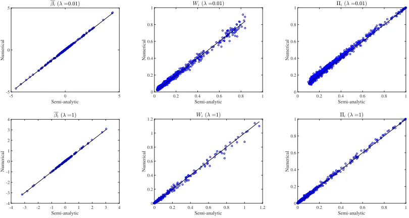
Figure 1 shows the plots of the experimental values of the quantities{βi, Wi,Πi}iagainst
their semi-analytic counterparts for the non-random penalty casew= 1 with the bootstrap resampling τ = 1, which is the situation considered in Bolasso. The same plots in the SS situation, w= 0.5(<1), pw = 0.5, and τ = 0.5, are shown in Figure 2. Other detailed
pa-rameters are provided in the captions. These results show that the proposed semi-analytic
-5 0 5
Semi-analytic -5
0 5
Numerical
0 0.2 0.4 0.6 0.8 1
Semi-analytic 0
0.2 0.4 0.6 0.8 1
Numerical
0 0.2 0.4 0.6 0.8 1
Semi-analytic 0
0.2 0.4 0.6 0.8 1
Numerical
-4 -3 -2 -1 0 1 2 3 4
Semi-analytic -4
-3 -2 -1 0 1 2 3 4
Numerical
0 0.2 0.4 0.6 0.8 1 1.2
Semi-analytic 0
0.2 0.4 0.6 0.8 1 1.2
Numerical
0 0.2 0.4 0.6 0.8 1
Semi-analytic 0
0.2 0.4 0.6 0.8 1
Numerical
Figure 1: Experimental values of βi (left), Wi (middle), and Πi (right) are plotted against
those computed by the semi-analytic method in the non-random penaltyw = 1 and τ = 1 case. The upper panels are for λ= 0.01 and the lower are for λ= 1. The other parameters are set to be (N, α, ρ0, σξ2) = (1000,0.5,0.2,0.01).
method reproduces the numerical results fairly accurately. As far as it was examined, re-sults of similar accuracy were obtained for a very wide range of parameters. These validate the proposed semi-analytic method.
-3 -2 -1 0 1 2 3
Semi-analytic
-3 -2 -1 0 1 2 3
Numerical
0 0.5 1 1.5 2 2.5 3 3.5 4 Semi-analytic
0 0.5 1 1.5 2 2.5 3 3.5 4
Numerical
0 0.2 0.4 0.6 0.8
Semi-analytic 0
0.1 0.2 0.3 0.4 0.5 0.6 0.7 0.8 0.9
Numerical
-1 -0.5 0 0.5 1
Semi-analytic
-1 -0.5 0 0.5 1
Numerical
0 0.5 1 1.5 2 2.5
Semi-analytic
0 0.5 1 1.5 2 2.5
Numerical
0 0.1 0.2 0.3 0.4 Semi-analytic 0
0.05 0.1 0.15 0.2 0.25 0.3 0.35 0.4 0.45
Numerical
Figure 2: Same plots as in Figure 1 in the random penalty case with w = 0.5, pw = 0.5,
and τ = 0.5. The parameters of each panel are identical to the corresponding parameters in Figure 1. In comparison to Figure 1,|βi|and Πitend to be smaller,
whereas Wi tends to be larger. This is probably due to the additional
This implies that a rather tight threshold is required for microscopic quantities such as βi
and Wi. Unless explicitly mentioned, this value = 10−10is used below.
4.1.2. Comparison with state evolution
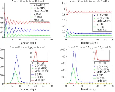
To examine the convergence properties of AMPR, we next see the dynamical behavior of the macroscopic quantities ( ˜χ(t),W˜(t),MSE(t)) as the algorithm steptproceeds, in compar-ison with the SE equations (36). Figure 3 shows the plots of them against t for different parameters. In all the cases, these macroscopic quantities rapidly take stable values and
0 5 10 15 20 25 30
Iteration step t
0 0.2 0.4 0.6 0.8 1 1.2
0 5 10 15 20 25 30
Iteration step t
0 0.2 0.4 0.6 0.8 1 1.2
0 5 10 15 20 25 30
Iteration step t 0
500 1000 1500 2000
0 10 20
0 10 20
0 5 10 15 20 25 30
Iteration step t 0
200 400 600 800 1000
0 10 20
0 5
Figure 3: Dynamical behavior of macroscopic parameters ( ˜χ(t),W˜(t),MSE(t)) initialized at ( ˜χ(0),W˜(0)) = (0,0) and MSE(0) ≈ 1. The result computed by SE is denoted by lines while the one by AMPR is represented by markers, and the agreement is fairly good. (Left) The non-randomized penalty case (w = 1, pw = 0, τ = 1).
(Right) The randomized penalty case (w=pw=τ = 1/2). The upper panels are
forλ= 1, while the lower ones are ofλ= 0.01 for which insets are given to show the MSE values in visible scales. The AMPR result is obtained at N = 20000. The other parameters are fixed at (α, ρ0, σ2ξ) = (0.5,0.2,0.01).
with the SE result by just one sample of {β0, X,ξ}, the model dimensionalityN is chosen as a rather large value of N = 20000 in the AMPR experiment. Although in Figure 3 the initial condition is fixed at χ(0) = W(0) =β(0) =0 corresponding to ( ˜χ(0),W˜(0)) = (0,0) and MSE(0) ≈1, we also examined several other initial conditions and confirmed the good agreement between the AMPR and SE results in all the cases.
4.1.3. Application to Bolasso
Bolasso is a variable selection method utilizing the positive probability (23) evaluated by the bootstrap resampling τ = 1 with no penalty randomization w = 1. Its soft version, abbreviated as Bolasso-S (Bach, 2008), selects variables with Πi ≥0.9 as active variables
and other variables are rejected from the support. We here adopt this manner and see the performance of AMPR used for implementing this.
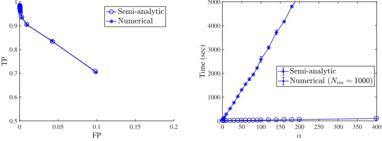
The left panel of Figure 4 shows the plot of the true positive ratio (TP) against the false positive ratio (FP) as the values of α change. Bolasso requires scaling the regular-ization parameter as λ∝ √α, and here, it is set to λ = (1/2)√α. The other parameters are fixed at (N, ρ0, σ2ξ) = (1000,0.2,0.01). As was theoretically shown (Bach, 2008), TP converges to unity, whereas FP tends to zero in this setup. This demonstrates that the
0 0.05 0.1 0.15 0.2 FP
0.5 0.6 0.7 0.8 0.9 1
TP
0 50 100 150 200 250 300 350 400
0 1000 2000 3000 4000 5000
Time (sec)
Figure 4: Bolasso experiment at (N, ρ0, σ2ξ) = (1000,0.2,0.01). The semi-analytic result (circle) is plotted with the numerical resampling result (asterisk). (Left) TP is plotted against FP asαincreases: TP approaches unity, whereas FP tends to zero. The semi-analytic result completely overlaps that of the numerical resampling. Error bars are omitted for clarity. (Right) Computational time plotted against
α. The observed large difference is attributed to the numerical resampling cost.
model consistency in the variable selection context is recovered. The contribution of this study is a significant reduction of the computational time: In the right panel, the actual computational time is compared between the semi-analytic method using AMPR and the direct numerical resampling, by plotting it against α. The computational costs of AMPR and Glmnet are both scaled asO(N M) and thus should be scaled linearly with respect to
compu-tational time is fully attributed to the numerical resampling cost. This demonstrates the efficiency of AMPR. It should be noted that the average over 10 different samples of D is taken in Figure 4 to obtain smooth curves and error bars.
4.1.4. Application to stability selection
SS is another variable selection method utilizing positive probability. The difference from Bolasso is the presence of the penalty coefficient randomization (w <1) and thatτ is set to 0.5. These introduce a further stochastic variation in the method, and consequently they tend to show a clearer discrimination in the positive probabilities between the variables in and outside the true support. AMPR can easily implement this, and here, it is compared with numerical resampling.
Figure 5 shows the plots of the positive probability values against λ, the so-called sta-bility path (Meinshausen and B¨uhlmann, 2010), and the computational time for obtaining the stability path against the covariate dimensionality N. The other parameters are fixed at (α, ρ0, σ2ξ, w, pw) = (2,0.2,0.01,0.5,0.5). Drawing all stability paths {Πi}i leads to an
10-2 10-1 100 101
0 0.2 0.4 0.6 0.8 1
Positive probabilities
102 103 104
100
101
102
103
104
105
Time (sec)
Figure 5: SS experiment at (α, ρ0, σξ2, w, pw) = (2,0.2,0.01,0.5,0.5). The semi-analytic
re-sult (circle) is plotted with the numerical resampling rere-sult (asterisk). (Left) Plots of the medians (points) and q-percentiles (bars) of {Πi}i∈S0 (TP) and {Πi}i /∈S0
(FP) with q = 16 and 84 againstλ forN = 8000. The semi-analytic result well overlaps that of the numerical resampling. There is a clear gap between TP and FP, suggesting that an accurate variable selection is possible. (Right) Computa-tional time plotted againstN on double-logarithmic scale. The dominant reason for the difference is again the numerical resampling cost.
unclear plot; thus, only the median andq-percentiles of {Πi}i∈S0 and those of {Πi}i /∈S0 are
B¨uhlmann (2010). The right panel shows a plot of the computational time by AMPR and by the numerical resampling. Both are supposed to be scaled asO(N M =N2). Although such a scaling is not observed in the AMPR result, it is expected to appear for larger N. Again, a significant difference in computational time is present between the semi-analytic and the numerical resampling methods, demonstrating the effectiveness of the proposed method.
4.1.5. Correlated covariates
In the derivation of AMPR and the associated SE equations, the weakness of correlations between covariates is assumed, but this assumption does not necessarily hold in realistic situations. Hence, it is important to check the accuracy of results obtained by AMPR for datasets with correlated covariates. Here we numerically examine this point.
To introduce correlations into the simulated dataset described above in a systematic way, we generate our covariates{xi}Ni=1 in the following manner: As a common component we first generate a vector xcom ∈ RM each component of which is i.i.d. from N(0,1/N);
choose a number 0≤rcom<1 controlling the ratio of the common component and generate a binary vector mi each component of which independently takes 1 with probability rcom;
take another vector ˜xi ∈RM each component of which is i.i.d. fromN(0,1/N), and generate
a covariate vectorxias a linear combination betweenxcomand ˜xi with usingmi as a mask.
These operations can be summarized in the following equation:
xi =xcom◦mi(rcom) + ˜xi◦(1−mi(rcom)), (37)
where◦ denotes Hadamard (component-wise) product. The covariates’ correlations mono-tonically increase asrcom grows. To quantify this, we compute an overlap between the co-variates, overlapij =x>i xj/
q
x>i xi
q
x>jxj
, and plot its mean value overiandj(6=i) in
Figure 6. Keeping in mind this quantitative information, we check the accuracy of AMPR below.
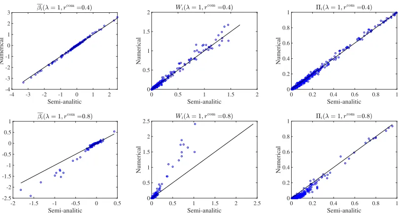
To directly see the accuracy of AMPR for correlated covariates, we plot the experimental values of the quantities {βi, Wi,Πi}i against those of AMPR in Figure 7 for two different
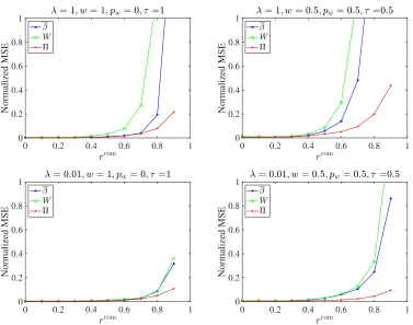
values of the common component ratio, rcom = 0.4 and rcom = 0.8. For rcom = 0.8, the AMPR result shows a clear deviation from the experimental one, while for rcom = 0.4 it still exhibits a good agreement with the experiment. Although Figure 7 is the specific result to the non-random penalty case (w = 1, τ = 1) with parameters (N, α, ρ0, σξ2, λ) = (1000,0.5,0.2,0.01,1), we have tested several different cases and observed similar tendency. To capture more global and quantitative information, we introduce a normalized MSE ofβ
between the experimentalβexp and AMPR βAMPR values as
PN
i=1
βexpi −βAMPRi 2 PN
i=1
βAMPRi
2 . (38)
0 0.2 0.4 0.6 0.8 1 0
0.2 0.4 0.6 0.8 1
Mean overlap
Figure 6: Plot of mean overlap of covariates against the common component ratio rcom. This is a result of a single numerical simulation at (N, α) = (1000,0.5), but the invariability of the result against changing the parameters has been also checked.
-4 -3 -2 -1 0 1 2
Semi-analitic -4
-3 -2 -1 0 1 2 3
Numerical
0 0.5 1 1.5 2
Semi-analitic 0
0.5 1 1.5 2
Numerical
0 0.2 0.4 0.6 0.8 1
Semi-analitic
0 0.2 0.4 0.6 0.8 1
Numerical
-2 -1.5 -1 -0.5 0 0.5
Semi-analitic -2.5
-2 -1.5 -1 -0.5 0 0.5 1
Numerical
0 0.5 1 1.5 2 2.5
Semi-analitic 0
0.5 1 1.5 2 2.5
Numerical
0 0.2 0.4 0.6 0.8 1
Semi-analitic
0 0.2 0.4 0.6 0.8 1
Numerical
Figure 7: Experimental values of βi (left), Wi (middle), and Πi (right) are plotted against
those computed by AMPR for correlated covariates withrcom= 0.4 (upper) and
0 0.2 0.4 0.6 0.8 1 0
0.2 0.4 0.6 0.8 1
Normalized MSE
0 0.2 0.4 0.6 0.8 1
0 0.2 0.4 0.6 0.8 1
Normalized MSE
0 0.2 0.4 0.6 0.8 1
0 0.2 0.4 0.6 0.8 1
Normalized MSE
0 0.2 0.4 0.6 0.8 1
0 0.2 0.4 0.6 0.8 1
Normalized MSE
Figure 8: Plots of normalized MSEs of β, W,Π against rcom of the non-randomized (left,
w= 1, pw = 0, τ = 1) and randomized (right, w=pw =τ = 1/2) penalty cases.
cases are presented, with two different values ofλ. This suggests that AMPR is practically reliable up to a certain level of correlations: For example ifrcom≤0.6, the normalized MSE of β is well suppressed and is commonly less than 0.2. According to Figure 6, rcom = 0.6 corresponds to the mean overlap value of about 0.36 which is not small. This speaks for the effectiveness of AMPR even for real-world datasets, as long as the correlations are not too large.
The above discussion clarifies the accuracy of AMPR for correlated covariates, but a more crucial issue is in its convergent property. For the non-correlated case of rcom = 0, AMPR converges very rapidly as shown in Figure 3, but for correlated cases it tends to badly converge and can even diverge. A common way to overcome this is to introduce a damping factor γ in the update (Caltagirone et al., 2014; Rangan et al., 2014), and we adopted this in the above experiments. The update with the damping factor can be symbolized as
θ(t+1)= (1−γ)θ(t)+γG(θ(t)), (39)
whereθ is a variable summarizing (β,χ,W) andGrepresents the AMPR operations. The original message passing update corresponds toγ = 1. Smaller values ofγ are better for the stability of the algorithm but takes a longer time until the convergence. Our experiments on the simulated dataset seemingly show that a smaller value ofγ is needed for largerrcom
and smaller λ. For example for obtaining Figure 7, we needed to set γ <0.1 for avoiding divergence. This value is found experimentally, and it is desired to find a more principled way to choose an appropriate value of γ or a more effective way to better control the convergence of AMP type algorithms. Some earlier studies tackled this problem (Caltagirone et al., 2014; Rangan et al., 2014), but the complete understanding of the convergent property is still missing. Investigation along this direction is an important topic but is beyond the purpose of the present paper.
4.2. Real-world dataset
In this subsection, AMPR is applied to a real-world dataset, and the stability path is computed for examining the relevant covariates or variables. The dataset treated here is the wine quality dataset (Lichman, 2013): The data size is M = 4898 (only white wine is treated), and the number of covariates, which represent physicochemical aspects of wine, is N0 = 11. The basic aim of this dataset is to model wine quality in terms of the physicochemical aspects only, and the response is an integer-valued quality score from zero to ten obtained by human expert evaluation. This dataset can be used in both classification and regression, and the linear model was also tested in earlier studies (Cortez et al., 2009; Melkumova and Shatskikh, 2017). Lasso and SS are applied to this dataset.
As preprocessing,Nnoisenoise variables are added into the dataset. Each component of the noise variables is i.i.d. from N(0,1/N). The usual standardization, zeroing the mean of all variables and responses and normalizing the variables to be of unit norm, is also conducted.
resolving the arbitrariness of judging criterion of the positive probability both in Bolasso and SS. As far as we have searched, this kind of active construction of rejection regions has never been observed in literatures, and hence this proposition itself can be regarded as a part of new results of this paper.
This sort of manipulation to dataset is usually unfavored because it increases the com-putational cost and tends to contaminate the dataset. However thanks to AMPR, the first computational issue becomes less serious since the computational time of AMPR increases just linearly with respect to the number of added noise variables Nnoise. The second issue does not seem to be serious either for the wine quality dataset, because the dataset size
M = 4898 is very large compared to the number of original variablesN0 = 11. Below, we experimentally check if this strategy works well or not.
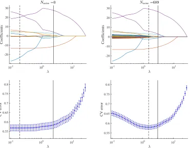
Let us start from checking how the noise variables influence on the dataset. To this end, we plot the solution paths and the generalization errors estimated by 10-fold cross validation (CV) in Figure 9 in the cases with and without the noise variables. This figure
10-1 100 101
-20 -10 0 10 20 30
Coefficients
10-1 100 101
-20 -10 0 10 20 30
Coefficients
10-1 100 101
0.55 0.6 0.65 0.7 0.75 0.8
CV error
10-1 100 101
0.55 0.6 0.65 0.7 0.75 0.8
CV error
Figure 9: Solution paths (top) and CV errors plotted against λ(bottom), for Nnoise = 0 (left) and Nnoise = 689 (right). The vertical dotted line denotes the location of the CV error minimum, λmin, whereas the vertical straight line represents the location selected by the one-standard-error rule that “defines” the optimalλ
Table 1: Overlap of the 3rd covariate (citric acid) and the others
index i 1 2 3 4 5 6 7 8 9 10 11
overlapx>
i x3 0.29 -0.15 1.00 0.09 0.11 0.09 0.12 0.15 -0.16 0.06 -0.07
indicates that the solution paths of the original variables and the CV error value are stable against the introduction of noise variables, particularly in the relevant range of λ. At the optimalλ(λopt), chosen by the one-standard-error rule (Trevor et al., 2009), the variables in the support are common in both cases: They are indexed as 1,2,4,5,6,10, and 11, which represent fixed acidity, volatile acidity, residual sugar, chlorides, free sulfur dioxide, sulphates, and alcohol, respectively. Hence, we can conclude that the introduction of the noise variables hardly affects the estimates of the original variables, and we can effectively use the noise variables to judge the significance of each original variable.
Subsequently, the result of applying SS with (τ, w, pw) = (0.5,0.5,0.5) to this dataset is
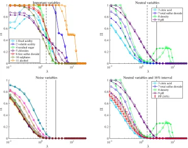
examined. Figure 10 shows the plots of the stability paths according to the three categories of variables: The “important” variables are defined as being in the support, at λopt in the Lasso analysis, and thus their indices are 1,2,4,5,6,10,11; the “neutral” variables are the other variables in the original dataset, and the corresponding indices are 3,7,8,9; the remaining are the noise variables. Both the results of AMPR (circle) and the direct numerical resampling (asterisk) are shown (the same variable is depicted in the same color). Consequences of Figure 10 are three-fold. The first one is consistent agreement between the results of AMPR and the direct numerical resampling. For all categories, the two curves of each stability path Πi(λ) by AMPR and the direct numerical resampling are very close
to each other. This is an additional evidence supporting the accuracy of the proposed semi-analytic method in real-world datasets with correlated covariates. The computational time for obtaining these results in an experiment is 1077 s by AMPR and 2859 s by the numerical resampling, demonstrating the efficiency of AMPR. It should be stressed that this efficiency can be enhanced by optimizing the implementation of AMPR. The second consequence is the different behaviors of stability paths in different categories. The positive probabilities of the important variables (upper left) are growing largely even forλ > λmin, while those of the noise variables (lower left) do not grow well unlessλdrops belowλmin. The behavior of the neutral variables (upper right) is somewhat elusive, and a better interpretation is provided by utilizing the noise variables, which is the third consequence: As discussed above, we can define a rejection region from the distribution of stability paths of the noise variables; an actual definition here is theq-percentiles withq= 16 and 84 of the distribution, which is in the lower right panel depicted by red bars with the median (red markers) of the distribution, the legend of which is given as FP, in the same manner as Figure 5. This analysis shows that citric acid and total sulfur dioxide of the neutral variables tend to be in the rejection region, implying that they are irrelevant for modeling wine quality. Moreover, density and pH are well beyond the interval of the rejection region, and they can be regarded as relevant, even though the behavior of density’s path is rather tricky.
10-1 100 101 0
0.2 0.4 0.6 0.8
1 Important variables
1 fixed acidity 2 volatile acidity 4 residual sugar 5 chlorides 6 free sulfur dioxide 10 sulphates 11 alcohol
10-1 100 101
0 0.2 0.4 0.6 0.8
1 Neutral variables
3 citric acid 7 total sulfur dioxide 8 density 9 pH
10-1 100 101
0 0.2 0.4 0.6 0.8 1
Noise variables
10-1 100 101
0 0.2 0.4 0.6 0.8
1 Neutral variables and 16% interval 3 citric acid 7 total sulfur dioxide 8 density 9 pH FP (16%)
with several others, particularly with the 1st variable. This implies that citric acid can be replaced by the 1st variable or fixed acidity. This is a plausible explanation because the proposed model puts considerably more weight on fixed acidity than on citric acid, whereas the opposite is the case in Cortez et al. (2009). Further thorough comparison will be required to determine which model is better.
Table 1 also implies why AMPR works well for the wine quality dataset: The maximum value of the covariates’s overlap is about 0.29 which corresponds rcom ≈ 0.5 in Figure 6; Figure 8 shows that the accuracy of AMPR is commonly good around that value of rcom, explaining the accuracy of AMPR. This consideration indicates that given a new dataset we can judge whether AMPR will give an accurate result or not for the dataset from the covariates’ overlap and Figures 6 and 8.
Overall, the analysis using stability paths provides richer information that cannot be obtained by solely using Lasso. A new objective criterion could be proposed for determin-ing the relevance of variables by utilizdetermin-ing the distribution of stability paths of the added noise variables. These facts highlight the effectiveness of the resampling strategy in vari-able selection, and the proposed semi-analytic method can implement this strategy in a computationally efficient manner.
5. Conclusion
An approximate method was developed for performing resampling in Lasso in a semi-analytic manner. The replica method enables us to semi-analytically take the resampling av-erage over the given data and the avav-erage over the penalty coefficient randomness, and the resultant replicated model is approximately handled by a Gaussian approximation us-ing the cavity method. A message passus-ing algorithm named AMPR is thus derived, the computational cost of which is O(N M) per iteration and is sufficiently reasonable. Its convergence in O(1) iterations is guaranteed by a state evolution analysis when covariates are given as zero-mean i.i.d. Gaussian random variables. We demonstrated how it actually works through numerical experiments using simulated and real-world datasets. Comparison with direct numerical resampling has evidenced its approximation accuracy and efficiency in terms of computational cost, even for covariates with correlations of a moderate level. AMPR was also employed to approximately perform Bolasso and SS, and it was applied to the wine quality dataset (Lichman, 2013; Cortez et al., 2009). To provide a finer quan-titative analysis of the dataset, an objective criterion was proposed for determining the relevance of the stability paths by processing the added noise variables, yielding reasonable results in satisfactory computational time.
An advantage of the present framework is its generality. For example, its extension to a generalized linear model is straightforward. This is an immediate future research direction. Extensions to other resampling techniques, such as the multiscale bootstrap method (Shimodaira et al., 2004), would also be interesting.
sophisticated approximations, such as the expectation propagation or the adaptive TAP method (Opper and Winther, 2001a,b, 2005; Kabashima and Vehkapera, 2014; C¸ akmak et al., 2014; Cespedes et al., 2014; Rangan et al., 2016; Ma and Ping, 2017; Takeuchi, 2017). Applying those approximations with retaining the benefit of message passing algorithms, the low computational cost, is still a nontrivial challenge and promising future work.
Resampling is a very versatile framework applicable to various contexts and models in statistics and machine learning. Reducing its computational cost by extending the present method will thus be beneficial in various fields, and can even be imperative, as available data in society will continue to increase rapidly.
Acknowledgement
This work was supported by JSPS KAKENHI Nos. 25120013 and 17H00764. TO is also supported by a Grant for Basic Science Research Projects from the Sumitomo Foundation. The authors thank Hideitsu Hino for useful comments.
References
Francis R Bach. Bolasso: model consistent lasso estimation through the bootstrap. In Proceedings of the 25th international conference on Machine learning, pages 33–40. ACM, 2008.
Onureena Banerjee, Laurent El Ghaoui, Alexandre d’Aspremont, and Georges Natsoulis. Convex optimization techniques for fitting sparse gaussian graphical models. In Pro-ceedings of the 23rd international conference on Machine learning, pages 89–96. ACM, 2006.
Jean Barbier, Nicolas Macris, Mohamad Dia, and Florent Krzakala. Mutual information and optimality of approximate message-passing in random linear estimation. arXiv preprint arXiv:1701.05823, 2017.
Mohsen Bayati and Andrea Montanari. The dynamics of message passing on dense graphs, with applications to compressed sensing. IEEE Transactions on Information Theory, 57 (2):764–785, 2011.
Francesco Caltagirone, Lenka Zdeborov´a, and Florent Krzakala. On convergence of approx-imate message passing. In 2014 IEEE International Symposium on Information Theory, pages 1812–1816, June 2014. doi: 10.1109/ISIT.2014.6875146.
Burak C¸ akmak, Ole Winther, and Bernard H Fleury. S-amp: Approximate message passing for general matrix ensembles. InInformation Theory Workshop (ITW), 2014 IEEE, pages 192–196. IEEE, 2014.
Paulo Cortez, Ant´onio Cerdeira, Fernando Almeida, Telmo Matos, and Jos´e Reis. Model-ing wine preferences by data minModel-ing from physicochemical properties. Decision Support Systems, 47(4):547–553, 2009.
David L Donoho, Arian Maleki, and Andrea Montanari. Message-passing algorithms for compressed sensing. Proceedings of the National Academy of Sciences, 106(45):18914– 18919, 2009.
Viktor Dotsenko. Introduction to the replica theory of disordered statistical systems, vol-ume 4. Cambridge University Press, 2005.
Bradley Efron and Robert J Tibshirani. An introduction to the bootstrap. CRC press, 1994.
Jerome Friedman, Trevor Hastie, and Robert Tibshirani. Sparse inverse covariance estima-tion with the graphical lasso. Biostatistics, 9(3):432–441, 2008.
Jerome Friedman, Trevor Hastie, and Rob Tibshirani. Regularization paths for generalized linear models via coordinate descent. Journal of statistical software, 33(1):1, 2010.
Max Grazier G’Sell, Jonathan Taylor, and Robert Tibshirani. Adaptive testing for the graphical lasso. arXiv preprint arXiv:1307.4765, 2013.
Edwin Hewitt and Leonard J Savage. Symmetric measures on cartesian products. Trans-actions of the American Mathematical Society, 80(2):470–501, 1955.
Adel Javanmard and Andrea Montanari. Confidence intervals and hypothesis testing for high-dimensional regression. The Journal of Machine Learning Research, 15(1):2869– 2909, 2014a.
Adel Javanmard and Andrea Montanari. Hypothesis testing in high-dimensional regression under the gaussian random design model: Asymptotic theory. IEEE Transactions on Information Theory, 60(10):6522–6554, 2014b.
Adel Javanmard and Andrea Montanari. De-biasing the lasso: Optimal sample size for gaussian designs. arXiv preprint arXiv:1508.02757, 2015.
Yoshiyuki Kabashima. A cdma multiuser detection algorithm on the basis of belief propa-gation. Journal of Physics A: Mathematical and General, 36(43):11111, 2003.
Yoshiyuki Kabashima and Mikko Vehkapera. Signal recovery using expectation consistent approximation for linear observations. In Information Theory (ISIT), 2014 IEEE Inter-national Symposium on, pages 226–230. IEEE, 2014.
Keith Knight and Wenjiang Fu. Asymptotics for lasso-type estimators. Annals of statistics, pages 1356–1378, 2000.
M. Lichman. UCI machine learning repository, 2013. URLhttp://archive.ics.uci.edu/ ml.