Classification with multiple prototypes

MURDOCH RESEARCH REPOSITORY

http://dx.doi.org/10.1109/FUZZY.1996.551812

Bezdek, J.C., Reichherzer, T.R., Lim, G. and Attikiouzel, Y.

(1996) Classification with multiple prototypes. In: Proceedings

of the Fifth IEEE International Conference on Fuzzy Systems, 8 -

11 September, New Orleans, USA, pp. 626-632.

http://researchrepository.murdoch.edu.au/19282/

Copyright © 1996 IEEE

Personal use of this material is permitted. However, permission to reprint/republish

this material for advertising or promotional purposes or for creating new collective

J a m e s C. Bezdek

Thomas R. Reichherzer

Department of Computer Science

University of West Florida

Pensacola, FL 32514, USA

Gek Lim

Yianni

Attikiouzel

Center for Intell. Inf. Proc. Systems

Dept.

of Electrical and

Electronic

Eng.

University of Western Australia

Nedlands, Perth,

6009,

Western Australia

act

We compare learning vector quantization, f u z z y learning vector quantization, and a

deterministic scheme called the dog-rabbit [OR) model f o r generation of multiple prototypes from labeled data f o r classifier design. We also compare these three models

to three other methods: a clumping method due to C . L. Chang; our modijkation of C.L. Chang’s method; and a derivative of the batch f u z z y c-means algorithm due to Yen and C.W. Chang. All six methods are

superior to the labeled subsample means, which yield 1 1 errors with 3 prototypes. Our modified Chang’s method is, for the Iris data used in this study, the best of the six schemes in one sense; it_finds 11 prototypes that yield a resubstitution error rate of 0. In

a different sense, the DR method is best, yielding a classifier that commits only 3 errors with 5 prototypes.

There are four types of class labels -

crisp, fuzzy, probabilistic and possibilistic. Let integer c denote the number of classes, 1

< c < n, and define three sets of label vectors in %‘as follows :

N = [0,1]‘ - {(0, 0,

.

. . O)T) ; (14

P C

y E Npc: i y i =I}

:

(1b) i = l

Nhc is the canonical (unit vector) basis of Euclidean c-space. The i-th vertex of Nhc ,

ei = (0, 0 ,..., 1 is the crisp

label for class i, 1 5 i 5

c.

Nfc , a piece of a hyperplane, is the convex hull of Nhc

.

The

vector y = (0.1, 0.6, 0.3)T is a fuzzy or probabilistic label vector: its entries lie between 0 and 1, and s u m to 1. The interpretation of y depends on its origin. If y is a label vector for some x E 9Ip generated by, say, the fuzzy c-means clustering method, we call y a fuzzy label for x. If y

came from a method such as maximum likelihood estimation in mixture decomposition, y would be a probabilistic label. N the unit hypercube in Sc, excluding the origin, contains possibilistic label vectors such as z = (0.7, 0.2, 0.7)T. Note that N,, c N, c N,,

.

,..., O)T,

-7

PC’

v

= {vl ,vg ,

. .

.

,

vc}

c 91p of prototypes (or

centers) for clusters in X from unlabeled object data are :

Label Model/ A 0 Algorithm

Ref.

Crisp Crisp c-means/ HCM 111 Fuzzy Fuzzy c-means/ FCM 121 Prob. Statistical mixture/EM [3] Poss. Poss. c-means/ PCM [41

Object data are represented as X = (xl ,

x2,

. . .

, xn} in feature space 531’. The k-th object ( a ship, patient, stock market report, pixel, etc.) has Xk as it’s numerical representation; x is the j-th characteristic (or feature) associated with object

k.

A

PC’

classLfier, any function D : %’I+ N

specifies c decision regions in 3’. Training a classifier means identification of the parameters of D if it is explicit: or representing t h e boundaries of D algorithmically if it is implicit. The value y

= D(z) is the label vector for z in 91p. D is a

crisp

classfier

if D[91p] = Nhc. New, unlabeled object data that enter feature space after crisp decision regions are defined simply acquire the label of the region they land in. If the classifier is fuzzy, probabilistic or possibilistic, labels (y) assigned to object vectors z during the operational (i.e., classification) phase are almost always converted to crisp ones through hardening of y with the function

jk

H(D(z)P = H(y) = ei

-

y i 2 y j ; j + i

In (2) the distance is Euclidean,

6,(y, e ) = IIy - ellI = J ( y - e)T(y - e)

.

If the design data are labeled, finding D is called supervised learning. Then X is usually crisply partitioned into a design ( o r training) set Xtr with label matrix Ltr; and a

test

set Xte = (X -

%r)

with label matrix Lte. Columns of Ltr and Lte are label vectors in N Testing a classifier D designed with

PC’

Xtr means: submit

%e

to D , and c mistakes (Lte must have crisp labels for data in

%e

in order to do this). This yields the apparent error rate ED(XteIXtr) ; our notation indicates that D was trained with X,,, and tested with Xte. ED is usually the performance index by which D is judged, and for convenience, we refer to it simply as the error rate. ED(XIX) is called the resubstitution error rate. Resubstitution uses the same data for training and testing, so it usually produces an optimistic error rate, but this is not a n impediment to using it to compare different designs.

If Xtr is large enough and its substructure is well delineated, we expect classifiers trained with it to yield small error rates. On the other hand, when the training data are large in dimension p and/or number a, classifiers such as the k-nearest neighbor (Dk-nn) rule [5,6] can require too much storage and CPU time for efficient deployment. Here we discuss 6 ways to replace Xtr with a set of prototypes V that can be used as a substitute for

%

(e.g., in the nearest neighbor rule) without appreciable degradation in E D ~ - ~ ~ : ( X ~ ~ I X d

.

In this case Dk-nn becomes a nearest prototype design with error rate ED(Xte I

V)

2. Nearest prototype classifiers

Once the prototypes

V

are found (and possibly relabeled if the data have physical labels), they can be used to define a crisp

nearest

prototype (1 -np) classifier, say Dv,6 :

The nearest prototype (1-np) Classifier.

Given a n y c prototypes V = (V.E 32’ : 12 j l c

J

} , one v. /class, and any dis-similarity J

measure 6 on 3’ : for any z E 3’:

Decide z E class i

Ties in (3) are arbitrarily resolved. The crisp 1-np design can be implemented using

prototypes from a n y algorithm that produces them. Equation (3) defines a crisp classifier, even when

V

comes from a fuzzy, probabilistic or possibilistic algorithm. When one or more classes are represented by multiple prototypes, there are two ways to extend the 1-np design. We can simply use equation ( 3 ) , recognizing that V contains more than one prototype for at least one of the c classes. Or we can extend the 1-np design to a k-np rule, wherein the k nearest prototypes are used to conduct a vote about the label that should be assigned to input z.

This amounts to operating the k-nn rule using prototypes (points built from the data) instead of neighbors (points in the data). We opt here for the simpler choice, which is formalized as the

The

nearest multiple prototype (1-nmp]

classifier. Given a n y Np prototypes

Pj

V = ( v i j E 9 1 P : l < i < c ; 1 1 j l n Pj

I

,where n

is the number of prototypes for class j ,

N, =

C n p j :

and a n y dis-similarity

measure

F

on

sp:

for any z E 9lP: C

]=1

Decide z E class i a D V , 6 ( ~ ) = e, tj 3 ~ ~ 1 1 , ..., n ]36(z,vis)<F(z,v )

Pi .it

V j f: i and t E 11, ...,

f (3')

nPjl

As in ( 3 ) , ties in (3') are resolved arbitrarily. We use the same notation for the 1-np and 1-nmp classifiers, relying on context to identify which one is being discussed. Now we are ready t o turn to methods for finding multiple prototypes.

3.

Three

seque

Sequential learning models update estimates at iterate (t-1) of the {vi) at iterate t (one iteration is one pass through

X)

upon presentation of an xk from X using the general form, i = 1, 2,

-..,

c:

Vi.t = Vi,t-l 4- aik,t(Xk - v i , t - l ) * (4)

(i) the subset of nodes that get updated at each iterate, and (ii) values of the

{aik,tl

.

LVQ updates only the winner (i.e., the vi

closest to

%)

at each input, whereas GLVQ-F and the DR algorithm may update all c nodes for each presentation of an input. The learning rate distribution for LVQ is well known:

(0 , r = 1 , 2 ,

...

c

:

r f i

i

In (5)

at

is usually initialized at some value in (0, l), and decreased linearly with t. The model underlying GLVQ-F contains LVQ as a subcase and is discussed extensively elsewhere [8]. The GLVQ-F update rule for the prototypes V at iterate t in the special (and simple) case m=2 uses the following learning rate distribution in equation (4) , i = 1, 2, ..., c:

GLVQ-F - _-

?k,t

As in (5),

at in (6)

- now one component of the learning rates {aik,J - is usually

proportional to l/t, and the constant (2c) is absorbed in it without loss.

Like GLVQ-F, the DR algorithm

[lo]

may update all c nodes for each input. Unlike GLVQ-F, the DR algorithm is not based on an optimization problem. Rather, its authors use intuitive arguments to establish the learning rate distribution for update equation (4) that is used by the DR model:

(A)

(B) , r = l , Z , . . . c ; r f i

:

i =

arg

min

x

- v ~ , ~ - ~

ik,t - k

Ill

Ill}

.(7)

where

The DR user must specify an initial distribution for the (fik,t 2 1) , and four constants : a rate ofchange offatigue factor

A f > O ; a maximum fatigue fM

:

a fence

radius

R,

> 0 , and an inhibition constant

A > 0. Suppose v ~ , ~ - ~ to be the winning

prototype with llxk -

11

>

R,.

AII c nodes

are updated using (7) in (4). Following this, the distance llxk

-

vi,t

11

is compared to

R~

If

llxk - Vi,tII <

R,,

the closest dog is now inside

the fence around

xk,

and is slowed down by

increasing its fatigue, f&,t t f i k , t - l + Af

.

This inhibits future motion of this prototype a little (relative to the other nodes), and it also encourages non-winners to look for other data to chase. Movement of (i.e., updating) the i-th prototype ceases when fik,t > f,. Thus, termination of

updating is done node by node.

Unlike Chang's method, none of the CL methods iust described uses the labels of points in X,r during t r a i n i n g to guide iterates towarkk a good

V.

Consequently, at the end of the learning phase the c prototypes have algorithmic labels that may or may not correspond to the physicd labels of Xtr. The relabeling algorithm uses Ltr to attach the most likely physical label

to each vi. Let d be the number of classes in X t r , labeled by t h e crisp vectors

{el, e2,

..

.

, e E } = N , Now define p.., i=1,2,

...,

d , j=1,2,

...,

c to be the percentage (as a decimal) of training data from class i closest to v. via the 1-np rule DV,6E

.

Define

the matrix P = [p..]. P has

C

rows in Nfc. and c columns pi in N P E

.

We assign label e. to vi

when H ( p i ) = e

.

The assignment is formalized as

-

9

J

9

J

j

and its error rate is computed and tabulated using the c x c confusion matrix C = [c..ll = [

9

# labeled class j I but were really class i].

4.

Numerical resullts

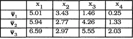
Following Chang [ 1 11, we use Anderson's Iris data 1121 as an experimental data set . Iris contains 50 (phyaically labeled) vectors in Cn4 for each of c=3 classes of Iris subspecies. For reference, the resubstitution error rate for the supervised 1-np design that uses the class means of each subset of Iris listed in Table 1 iiis single prototypes in (3) is 11 errors in 150 submissions using the Euclidean norm, ED- (Iris1 Iris) = 7.33%.

v , 6 E

I

I

x1

1

"2

I

x3

1

x4

1

v,

5.01 3.43 1.46 0.25

VQ 2.03

Table 1. Subsample (mean) prototypes

s4

for Iris

in

Computing protocols, control parameters, initialization, termination, iteration and robustness are discussed in ~ 4 1 .

I

I

Table 2. Typical confusion matrices and class representatives for 8 terminal prototypes

When the three CL algorithms are instructed to seek c = 8 prototypes, the error rate for all three 1-nmp designs typically remains a t 2.33% as shown in Table 2. Table 2 suggests that the replacement of

IFUS with 8 prototypes found by any of the three CL algorithms results in a 1-nmp design that is quite superior to the labeled

1-np design based on the c = 3 subsample means. Moreover, the DR model yielded consistently better results than either LVQ or GLVQ-F in almost every case we tested.

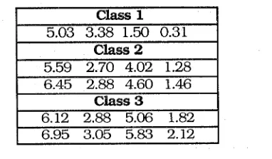
Table 3 reports best case results (as number of resubstitution errors) using each algorithm for various values of e. Shaded cells show the best case in each row. On passing from c = 3 to c = 4, even the best case error rate for all three models increased, followed by a decrease on passing from c = 4 to c = 5. One run of DR resulted in 5 prototypes t h a t produced only 3 resustitution errors when used in (3'). These prototypes are shown in Table 4.

Table 3. Number of resubstitution errors of the

1 -nmp designs : best case results

This shows that the Iris data can be well represented by five labeled prototypes. At the other extreme, increasing c past c = 8 has little effect on the best case results. Taken together, these observations suggest that Iris (and more generally, any labeled data set XI has some upper and lower bounds in terms of high quality representation by multiple prototypes for classifier design.

Table 4. Five DR prototypes that yield 3

resubstitution errors with the 1 -nmp rule on Iris

§

C.L. Chang's method begins by assuming every point in a labeled data set X is its own prototype, so let Vn = X. Consequently, the 1-np rule at (3) or the 1-nmp rule at (3') error rate is zero, EDvn,6E (XIV,) = 0. NOW

find (i, j) = arg min{[/lx,

-

- xtl\]}. Merge xi and

s t t

x. using vil = (Mx,

+

Nxj)/(M

+

N ) , where M and N are the number of merger parents of x i a n d x . respectively. Now s e t

Vn-l = X - {xi, xj]

+

vij and then calculate

(XIV,-l) using the 1-nmp rule at

(3'). If the error rate is still zero and if xi and x. have the same label , accept the merger and continue. If either (i) the error rate increases; or (ii) xi and x have different labels, do not merge xi and x.

.

In this case

J

Chang regards xi and x. as non-mergeable prototypes and continues. Note that when there is a merger, v.. automatically inherits the class label of its parents, and that the test data are fixed (all of X). Continue until further merging produces an error, and at this point stop, having found c prototypes

Vc that replace the n labeled data X and that preserve a resubstitution error rate of zero, i.e., EDV,,6E (XIV,) = 0 . Chang reports in

[ 121 that his method finds c = 14 prototypes that replace Iris and preserve a zero resubstitution error rate. The prototypes were not listed in [ 1 11.

J

J

EDV,-l .6E

J

j

J

1J

We modified Chang's approach in two ways (cf. Appendix). First, instead of using the weighted mean vu = (Mx,

+

Nxj)/(M

+

N) to merge prototypes we used the simple arithmetic mean. Second, we altered the search for candidates to merge two ways. First, we partition the distance matrix into c submatrices blocked by common labels, and look for the minimum in each sublock. This eliminates candidate pairs with different labels. Then, we attempt to merge the minimum of label-matched pairs. If this fails (because the prototype produced by merger yields a n error), we look at the next

merger can be done: or (ii) no merger is possible. The algorithm terminates when (ii) occurs. This is an effective strategy because merging the closest points of the same label is sufficient, but not necessary in order to preserve the error rate at zero. These two simple modifications led to c = 11 prototypes that yield zero resubstitution error.

Yen and Chang [131 modifed the (batch) fuzzy c-means algorithm so that it can be used to produce multiple prototypes for each class by an algorithm they called MFCM-n, n = l , 2,3. The theory of their method is well discussed elsewhere, so we are content here to show their results on Iris. Specifically, Yen and Chang compare four outputs: (FCM, c=3, 16 errors ): (MFCM-1, c=3, 16 errors); (MFCM-2, c=5 with (1,2,2) labeled prototypes for classes (1,2,3), 14 errors): and their best result (MFCM-3, c=7, with (1,3,3) labeled prototypes for classes (1,2,3), 8 errors).

5.

Conclusions

and

discussion

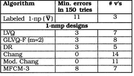
Table 5 summarizes the best results achieved by the seven algorithms used in our study. What does Table 5 entitle us to conclude? First, our results are of course specialized to j u s t one data set, and generalizations to other data warrant caution.

Table 5. Summary of the best error rates achieved by the 6 methods

All six 1-nmp designs use the labeled data more effectively than the 1-np design based on the labeled sample means. The minimum error rate (zero) is not realized by

the minimum number of prototypes (five). If

the determining criterion for choosing multiple prototypes is minimum error rate,

then our modification of Chang's method might be the method of choice. On the other hand, we can imagine applications (image compression comes to mind) where it is very important to find a minimum number of

prototypes

.

If this is important enough, developers may be willing to sacrifice a little accuracy to achieve this objective. In this case, the DR algorithm seems ideally suited to finding multiple prototypes that yield a few errors with fewer prototypes than the modified Chang's method.

Finally, we comment on the results reported by Yen and Chang [ 131. Their best 1 -nmp (batch-design) classifier was inferior to the best results achieved by all of the CL models. We suspect that sequential updating encourages "localized" prototypes which are able, when there is more than one per class, to position themselves better with respect to subclustei-s that may be present within the same clatss. This leads us to conjecture that batch algorithms are at their best when usedl to erect 1-np designs: and that sequential models are more effective for 1 -nmp classifiers.

6.

References

111 Duda, R. and Hart, P. (1973). P a t t e r n Classification and Scene Analysis, Wiley Interscience, NY.

[2] Bezdek, J. C. and Pal, S.K. (1992). Fuzzy Models for Pattern Recognition, lEEE Press, Piscataway, N J .

[3] Titterington, D., Smith, A. and Makov, U.

(1985). Statistical Analysis of Finite Mixture Distributions, Wiley, NY.

[4] Krishnapuram, R. and Keller, J. (1993). A Possibilistic Approach to Clustering, IEEE Trans. Fuzzy Systtvns, 1(2), 98-110.

[5] Dasarathy, B.V. ( 1 990). Nearest Neighbor (NN) Norms: NN Pattern Classification Techniques. IEEE Computer Society Press, Los Alamitos, CA.

161 Devijver, P. and Kittler, J. (1982).Pattern Recognition: A Statistical Approach, Prentice-Hall, Englewood Cliffs, N J .

[ 71 Kohonen, T. (198!3). Self-organization and Associative Memory. Springer-Verlag, Berlin, Germany, 3rd ed.

[8] Karayiannis, N., Bezdek, J.C., Pal, N.R., Hathaway, R.J. and Pai, P. (1995). Repairs to GLVQ : A new family of competitive learning schemes, in press, IEEE Trans. Neural Networks,.

[9] Pal, N.R., Bezdek, J.C., Tsao, E.C. (1993). Generalized Clustering Networks and Kohonen's Self-organizing Scheme. IEEE

Trans. Neural Networks.

(101 Lim. G.S., Alder, M. and Hadingham, P. (1992). Adaptive quadratic neural nets, Patt. Recog. Letters, 13, 325-329.

pen&.

The modified Chang

algorit

Store

Pick

rnitialize

[ l 11 Chang, C.L. (1974). Finding prototypes for nearest neighbor classification, IEEE Trans. Comp., 23( 1 1).

[12] Anderson, E. (1935). The IRISes of the Gaspe peninsula, Bull. Amer. IRIS Soc. , 59, 2-5.

[131 Yen, J. and Chang, C.W. (1994). A multi-prototype fuzzy c-means algorithm, Proc. 2nd EUFIT, Aachen, 539-543.

[14] Bezdek, J. C., Reicherzer, T. , Lim, G. and Attikiouzel, Y. (1995). Multiple prototype classifier design, in review, IEEE Trans. SMC.

c 6, (x, v) = IIx - vII, = d(x - v ) ~ (x - v) for similarity of data to prototypes

V,

t X ; EVn,6E (XIV,) = 0

While EV,,6E (XIV,) = 0 :

0 Compute the partitioned upper triangular distance matrix

Class 1 Class c

0 Find

(7,

;*)

= arg min [ilvf - vfll}, Compute vk* = (vk*

+

vf')/2, and update

L I

V L - ~

c

v,

-{vi k* , V, k*

I

+v*. If E ~ ~(XIVL-l) - ~=

o

, : ~

v ~ - ~

~ c compute

D(VnF1) ; continue.

Else return t o D(Vn) and find the next pair

(y,?*)

that solves

(

h* i , h*

)

=

-

argmin {IIv$ -vtll} and

(

h* i ,

)

#

( y ,

!*).

A t t e m p t to merge

vh* = (vp*

+

vy*)/2. Repeat step 0 until no merger is possible.