The Thirty-Third AAAI Conference on Artificial Intelligence (AAAI-19)
Machine Teaching for Inverse
Reinforcement Learning: Algorithms and Applications
Daniel S. Brown, Scott Niekum
Department of Computer ScienceUniversity of Texas at Austin {dsbrown,sniekum}@cs.utexas.edu
Abstract
Inverse reinforcement learning (IRL) infers a reward function from demonstrations, allowing for policy improvement and generalization. However, despite much recent interest in IRL, little work has been done to understand the minimum set of demonstrations needed to teach a specific sequential decision-making task. We formalize the problem of finding maximally informative demonstrations for IRL as a machine teaching problem where the goal is to find the minimum number of demonstrations needed to specify the reward equivalence class of the demonstrator. We extend previous work on algorithmic teaching for sequential decision-making tasks by showing a reduction to the set cover problem which enables an efficient approximation algorithm for determining the set of maximally-informative demonstrations. We apply our proposed machine teaching algorithm to two novel applications: providing a lower bound on the number of queries needed to learn a policy using active IRL and developing a novel IRL algorithm that can learn more efficiently from informative demonstrations than a standard IRL approach.
1
Introduction
As robots and digital personal assistants become more preva-lent, there is growing interest in developing algorithms that allow everyday users to program or adapt these intelligent sys-tems to accomplish sequential decision-making tasks, such as performing household chores, or carrying on a meaningful conversation. A common way to teach sequential decision-making tasks is through Learning from Demonstration (LfD) (Argall et al. 2009), in which the goal is to learn a policy from demonstrations of desired behavior. More specifically, Inverse Reinforcement Learning (IRL) (Ng and Russell 2000; Arora and Doshi 2018) is a form of LfD that aims to infer the reward function that motivated the demonstrator’s behavior, allowing for reinforcement learning (Sutton and Barto 1998) and generalization to unseen states. Despite much interest in IRL, there is not a clear, agreed-upon definition of optimality in IRL, namely, the size of the minimal set of demonstrations needed to teach a sequential decision-making task.
There are many compelling reasons to study optimal teach-ing for IRL: (1) it gives insights into the intrinsic difficulty of teaching certain sequential decision-making tasks; (2) it
Copyright c2019, Association for the Advancement of Artificial Intelligence (www.aaai.org). All rights reserved.
provides a lower bound on the number of samples needed by active IRL algorithms (Lopes, Melo, and Montesano 2009; Brown, Cui, and Niekum 2018); (3) optimal teaching can be used to design algorithms that better leverage highly informa-tive demonstrations which do not follow the i.i.d. assumption made by many IRL algorithms; (4) studying optimal teaching can help humans better teach robots through demonstration (Cakmak and Lopes 2012) and help robots better commu-nicate their intentions (Huang et al. 2017); and (5) optimal teaching can give insight into how to design (Mei and Zhu 2015) and defend against (Alfeld, Zhu, and Barford 2017) demonstration poisoning attacks in order to design IRL algo-rithms that are robust to poor or malicious demonstrations.
We formulate the problem of optimal teaching for se-quential decision making tasks using the recently popu-larizedmachine teachingframework (Zhu 2015). The ma-chine teaching problem is the inverse of the mama-chine learn-ing problem. In machine teachlearn-ing, the goal is to select the optimal training set that minimizes teaching cost, of-ten defined as the size of the training data set, and the loss or teaching risk between the model learned by the stu-dent and the learning target. While machine teaching has been applied to regression and classification (Zhu 2015; Liu and Zhu 2016), little work has addressed machine teach-ing for sequential decision-makteach-ing tasks such as learnteach-ing from demonstration via IRL.
The contributions of this paper are fourfold: (1) a formal definition of machine teaching for IRL, (2) an efficient algo-rithm to compute optimal teaching demonstrations for IRL, (3) an application of machine teaching to find the lower bound on the number of queries needed to learn a task using active IRL, and (4) a novel Bayesian IRL algorithm that learns more efficiently from informative demonstrations than a standard IRL approach by leveraging the non-i.i.d. nature of highly informative demonstrations from a teacher.
2
Related work
use submodularity to find an efficient approximation algo-rithm for an optimal teaching problem that has a set-cover reduction; however, their approach is designed for binary classification rather than sequential decision making.
Cakmak and Lopes (2012) examined the problem of giving maximally informative demonstrations to teach a sequential decision-making task; however, as we discuss in Section 5, their algorithm often underestimates the minimum number of demonstrations needed to teach a task. Other related ap-proaches examine how a robot can give informative demon-strations to a human (Huang et al. 2017), or formalize optimal teaching as a cooperative two-player Markov game (Hadfield-Menell et al. 2016); however, neither approach addresses the machine teaching problem of finding the minimum number of demonstrations needed to teach a task.
Our proposed machine teaching algorithm leverages the notion of behavioral equivalence classes over reward func-tions to achieve an efficient approximation algorithm. Zhang et al. (2009) also use behavioral equivalence classes over reward functions as part of their solution to a policy teaching problem, in which the goal is to induce a desired policy by modifying the intrinsic reward of an agent through incentives. Rathnasabapathy et al. (2006) and Zeng et al. (2012) use equivalence classes over agent behaviors when solving the problem of interacting with multiple agents in a POMDP.
There is a large body of work on using active learning for IRL (Lopes, Melo, and Montesano 2009; Cohn, Durfee, and Singh 2011; Cui and Niekum 2017; Sadigh et al. 2017; Brown, Cui, and Niekum 2018). Our goal of finding a min-imal set of demonstrations to teach an IRL agent is related to one of the goals of active learning: reducing the number of examples needed to learn a concept (Settles 2012). In ac-tive learning, the agent requests labeled examples to search for the correct hypothesis. Optimal teaching is usually more sample efficient than active learning since the teacher gets to pick maximally informative examples to teach the target concept to the learner (Zhu et al. 2018). Thus, a solution to the machine teaching problem for IRL provides a method for finding the lower bound on the number of queries needed to learn a policy when using active IRL.
In the field of Cognitive Science, researchers have investi-gated Bayesian models of informative human teaching and the inferences human students make when they know they are being taught (Shafto and Goodman 2008). Ho et al. (Ho et al. 2016) showed that humans give different demonstrations when performing a sequential decision making task, depend-ing on whether they are teachdepend-ing or simply dodepend-ing the task. While studies have shown that standard IRL algorithms can benefit from informative demonstrations (Cakmak and Lopes 2012; Ho et al. 2016), to the best of our knowledge, no IRL algorithms exist that can explicitly leverage the informative nature of such demonstrations. In Section 7.2 we propose a novel IRL algorithm that can learn more efficiently from informative demonstrations than a standard Bayesian IRL approach that assumes demonstrations are drawn i.i.d. from the demonstrators policy. Research in computational learn-ing theory has shown a dramatic reduction in the number of teaching examples needed to teach anticipatory learners who know they are being taught by a teacher (Doliwa et al. 2014;
Gao et al. 2017), but has not addressed sequential decision making tasks. To the best of our knowledge, our work is the first to demonstrate the advantages of an anticipatory IRL algorithm which can leverage the non-i.i.d. nature of highly informative demonstrations from a teacher.
3
Problem formalism
3.1
Markov decision processes
We model the environment as a Markov decision process (MDP),hS,A, T, R, γ, S0i, whereSis the set of states,Ais the set of actions,T :S × A × S →[0,1]is the transition function,R :S → Ris the reward function,γ ∈ [0,1)is
the discount factor, andS0 is the initial state distribution. A policyπ : S × A 7→ [0,1] is a mapping from states to a probability distribution over actions. We assume that a stochastic optimal policy gives equal probability to all optimal actions. The value of executing policy πstarting at states∈Sis defined as
Vπ(s) =E[
∞
X
t=0
γtR(st)|π, s0=s]. (1)
The Q-value of a state-action pair(s, a)is defined as
Qπ(s, a) =R(s) +γEs0∼T(·|s,a)[Vπ(s0)] (2)
and we denote the optimal Q-value function asQ∗(s, a) = maxπQπ(s, a).
As is common in the literature (Ziebart et al. 2008; Sadigh et al. 2016; Pirotta and Restelli 2016; Barreto et al. 2017), we assume that the reward function can be expressed as a linear combination of features,φ:S 7→Rk, so thatR(s) = wTφ(s)wherew∈Rkis the vector of feature weights. This
assumption is not restrictive as these features can be nonlinear functions of the state variables. We can write the expected discounted return of a policy as
ρ(π) = E[
∞
X
t=0
γtwTφ(st)|π] = wTµπ, (3)
whereµπ=E[P∞t=0γ
tφ(s t)|π].
3.2
Machine teaching
The machine teaching problem (Zhu 2015) is to select the optimal training set D∗ that minimizes the teaching cost, often defined as the size of the data set, and the teaching risk which represents the teacher’s dissatisfaction with the model learned by the student. We focus on the constrained form of machine teaching (Zhu et al. 2018) defined as
min
D TeachingCost(D) (4)
s.t. TeachingRisk(ˆθ)≤ (5)
ˆ
θ=MachineLearning(D) (6)
3.3
Problem definition
We now formulate the optimal teaching problem for IRL as a machine teaching problem. We assume that the expert teacher operates under a ground-truth reward,R∗, and is able to demonstrate state-action pairs(s, a)by executing the corresponding optimal policyπ∗. A naive formulation of the machine teaching problem for IRL would be to find the minimal set of demonstrations,D, that enables an IRL agent to learnR∗within someteaching risk. However, IRL is ill-posed (Ng and Russell 2000)—there are an infinite number of reward functions that explain any optimal policy. Instead, we focus on determining the minimal set of demonstrations that enable a learner to find a reward function that results in an optimal policy with performance similar to the performance of the teacher’s policy underR∗. Specifically, we define the policy loss of an estimated weight vectorwˆcompared with the true weight vectorw∗as
Loss(w∗,wˆ) =w∗T(µπ∗−µπˆ), (7)
whereπ∗is the optimal policy underw∗andˆπis the optimal policy underw. Equation (7) gives the difference in expectedˆ return between the teacher’s policyπ∗and the expected re-turn of the learner’s policy, when both are evaluated under the teacher’s reward functionR∗=w∗Tφ(s). We can now formalize the machine teaching problem for IRL.
Machine teaching problem for IRL: Given an MDP,M, and the teacher’s reward function,R∗=w∗Tφ(s), find the set of demonstrations,D, that minimizes the following opti-mization problem:
min
D TeachingCost(D) (8)
s.t. Loss(w∗,wˆ)≤ (9) ˆ
w=IRL(D) (10)
whereDis the set of demonstrations, andwˆ is the reward recovered by the learner using Inverse Reinforcement Learn-ing (IRL). This formalism covers both exact teachLearn-ing (= 0) and approximate teaching ( >0). In this work we define
TeachingCost(D) =|D| (11)
where,|D|can denote either the number of(s, a)pairs inD or the number of trajectories inD; however, our proposed approach can be easily extended to problems with different teaching costs, e.g., where some demonstrations may be more expensive or dangerous for the teacher.
3.4
Discussion
Like most machine teaching problems (Zhu et al. 2018), the machine teaching problem for IRL is a difficult optimization problem. A brute-force approach would require searching over the power set of all possible demonstrations. This search is intractable due to the size of the power set and the need to solve an IRL problem for each candidate set of demon-strations. One of our contributions is an efficient algorithm for solving the machine teaching problem for IRL that only requires solving a single policy evaluation problem to find
the expected feature counts ofπ∗and then running a greedy set-cover approximation algorithm.
Before discussing our proposed approach in detail, we first introduce the notion of a behavioral equivalence class which is a key component of our approximation algorithm. We will also provide an overview and analysis of the work of Cakmak and Lopes (2012) which provides the baseline and motivation for our approach.
4
Behavioral Equivalence Classes
Thebehavioral equivalence class(BEC) of a policyπis de-fined as the set of reward functions under whichπis optimal:BEC(π) ={w∈Rk |πoptimal w.r.t.R(s) =wTφ(s)}.
(12) In this section we briefly discuss how to calculate the be-havioral equivalence class for both a policy and for a set of demonstrations from a policy. Given an MDP with either finite or continuous states and with a reward function repre-sented as a linear combination of features, Ng and Russell (2000) derived the behavioral equivalence class (BEC) for a policy. We summarize their result as follows:
Theorem 1. (Ng and Russell 2000) Given an MDP, BEC(π) is given by the following intersection of half-spaces:
wT(µ(πs,a)−µ(πs,b))≥0, (13) ∀a∈arg max
a0∈AQ
∗(s, a0), b∈ A, s∈ S, (14)
wherew∈Rkare the reward function weights and
µ(πs,a)=E[ ∞
X
t=0
γtφ(st)|π, s0=s, a0=a], (15)
is the vector of expected feature counts that result from taking actionain statesand followingπthereafter.
We can similarly define the BEC for a set of demonstra-tionsDfrom a policyπ:
Corollary 1. BEC(D|π)is given by the following intersec-tion of half-spaces:
wT(µ(πs,a)−µπ(s,b))≥0, ∀(s, a)∈ D, b∈ A. (16)
All proofs can be found in the extended version of this paper (Brown and Niekum 2018b).
Example: Consider the grid world shown in Figure 1(a), with four actions available in each state and deterministic transitions. We computed the BEC using a featurized reward functionR(s) = wTφ(s), where w = (w0, w1)withw0
(a) Policy (b) BEC(Policy)
(c) Demonstration (d) BEC(Demonstration)
Figure 1: Behavioral equivalence classes (BEC) for a grid world with 6 states. The upper left state is a terminal state. Each state has 4 available actions and the reward function is a linear combination of two binary features that indicate whether the color of the cell is white or grey. (a) The optimal policy. (b) The resulting intersection of half-spaces (shaded region) that defines all weight vectors such that the policy shown in (a) is optimal. (c) A demonstration from the opti-mal policy in (a) that is not maxiopti-mally informative. (d) The intersection of half-spaces (shaded region) resulting from the demonstration shown in (c).
Figures 1(c) and 1(d) show the BEC of a demonstration. The demonstration shows that both feature weights are non-positive and that w1 is no better than w0 (otherwise the demonstration would have gone through the grey cell); how-ever, the demonstration leaves open the possibility that all feature weights are equal. However, if the demonstration had started in the top right cell, the BEC of the demonstration would be identical to the BEC of the optimal policy. This highlights the fact that some demonstrations from an opti-mal policy are more informative than others. An efficient algorithm for finding maximally informative demonstrations using the BEC of the teachers policy is one of the contribu-tions of this paper.
5
Uncertainty Volume Minimization
We now give an overview of the algorithmic teaching ap-proach proposed by Cakmak and Lopes (2012) which moti-vates our work. The main insight that Cakmak and Lopes use is that of Corollary 1: if an optimal demonstration contains
(s, a), then an IRL algorithm can infer that
Q∗(s, a)≥Q∗(s, b),∀b∈ A (17) ⇔ wT(µ(πs,a∗ )−µ
(s,b)
π∗ )≥0,∀b∈ A. (18) Given a candidate demonstration setD, Cakmak and Lopes use the intersection of the corresponding half-spaces (as de-fined in Corollary 1) as a representation of the learner’s un-certainty over the true reward function. They use a Monte
Carlo estimate of the volume of this cone as a measure of the learner’s uncertainty, and seek demonstrations that minimize the uncertainty,G(D), over the true reward function, where
G(D) = 1
N
N
X
j=1
δ(xj∈C(D)), (19)
δis an indicator function,C(D)is the intersection of half-spaces given in Corollary 1, and the volume is estimated by drawingN random pointsxjfrom[−1,1]k. The set of maximally informative demonstrations is chosen greedily by iteratively selecting the trajectory that maximally decreases
G(D). This process repeats untilG(D)falls below a user defined threshold. We refer to this algorithm as the Uncer-tainty Volume Minimization (UVM) algorithm.
In the UVM algorithm, trajectories are added untilG(D)
is below some user-provided threshold; however, this does not solve the machine teaching problem for IRL presented in Section 3.3. This is because it only ensures that the estimated uncertainty volumeG(D)is less than, not that the policy loss (Eq. (7)) is less than. In order to guarantee that the policy loss is below a desireable level, this threshold must be carefully tuned for every MDP. Ifis too low, then the algorithm will never terminate. Alternatively, ifis too high, then not enough demonstrations will be selected to teach an appropriate reward function and the policy loss may be large, depending on the reward function selected by the IRL algorithm. In our experiments we remove the need for param-eter tuning by stopping the UVM algorithm if it cannot add another demonstration that decreasesG(D).
Another limitation of the UVM algorithm is that of volume estimation: exact volume estimation is #P-hard (Valiant 1979; Simonovits 2003) and straightforward Monte Carlo estimation is known to fail in high-dimensions (Simonovits 2003). Additionally, if there are two (or more) actions that are both optimal in states, and those two actions (aandb) are demonstrated, this will result in the following constraints:
wT(µ(πs,a)−µ(πs,b))≥0 and wT(µ(πs,b)−µ(πs,a))≥0 ⇒wT(µ(s,b)
π −µ
(s,a)
π ) = 0 (20) This is problematic because any strict subspace ofRk has measure zero, resulting in an uncertainty volume of zero. Thus, the UVM algorithm will terminate with zero uncer-tainty if two optimal actions are ever demonstrated from the same state, even if this leaves an entire(k−1)dimensional subspace of uncertainty over the reward function. Note that whenπ∗is a stochastic optimal policy this behavior will oc-cur once any trajectory that contains a state with more than one optimal action is chosen—the best trajectory to select next will always be one that visits a previously demonstrated state and chooses an alternative optimal action, resulting in zero uncertainty volume.
to only use deterministic policies for teaching. We instead propose a novel approach based on a set cover equivalence which removes the need to estimate volumes and works for both deterministic and stochastic teacher policies.
6
Set Cover Machine Teaching for IRL
Our proposed algorithm seeks to remedy the problems with the UVM algorithm identified in the previous section in order to find an efficient approximation to the machine teaching problem proposed in Section 3.3.Our first insight is the following:
Proposition 1. Consider an optimal policyπ∗for reward
R∗(s) =w∗Tφ(s). Given any weight vectorw∈BEC(π∗), ifR(s) = wTφ(s)is not constant for all states inS, then Loss(w∗,w) = 0.
This proposition says that if we have a non-degenerate weight vector in the behavioral equivalence class for a policy
π∗, then we incur zero policy loss by usingwrather than w∗for performing policy optimization. This follows directly from Equation (12). Thus, to ensure that the policy loss con-straint, Loss(w∗,wˆ) ≤ , holds in the machine teaching problem, we can focus on finding a demonstration setDsuch that the weight vector,w, learned through IRL is in BEC(ˆ π∗).
Note that Proposition 1 also assumes that the IRL agent being taught will not find a degenerate reward function if a non-degenerate solution exists. This property is true of all standard IRL methods (Gao et al. 2012; Arora and Doshi 2018). While it is possible that an IRL algorithm may return a constant reward function (e.g.,R(s) = 0,∀s∈ S) ifD=∅, the only way forD=∅to be the optimal solution for machine teaching is if the resulting loss is less than, i.e.,
Loss(w∗,wˆ) =w∗T(µπ∗−µπˆ)≤. (21) For= 0, this will be false since a constant reward function will almost surely lead to an optimal policyˆπwhich does not match the feature counts of the teacher’s policy,π∗.
Our second insight is based on the fact that the behavioral equivalence class forπ∗is an intersection of half-spaces (The-orem 1). Rather than give demonstrations until the uncertainty volume,G(D), is less than some arbitrary value, demonstra-tions should be chosen specifically to define BEC(π∗). Thus, to obtain a feasible solution to the machine teaching prob-lem for IRL we need to select a demonstration set such that the corresponding intersection of half-spaces, BEC(D|π∗)is equal to BEC(π∗).
Our final insight is to formulate an efficient approxima-tion algorithm for the machine teaching problem for IRL through a reduction to the set cover problem. This allows us to avoid the difficult volume estimation problem required by the UVM algorithm and focus instead on a well known dis-crete optimization problem. From Section 4 we know that the behavioral equivalence class of both a policy and a demon-stration are both characterized by intersections of half-spaces, and each demonstration fromπ∗produces an intersection of half-spaces which contains BEC(π∗). Thus, the machine teaching problem for IRL (Section 3.3) with= 0is an in-stance of the set cover problem: we have a set of half-spaces defining BEC(π∗), each possible trajectory fromπ∗covers
zero or more of the half-spaces that define BEC(π∗), and we wish to find the smallest set of demonstrations,D, such that BEC(D|π∗) =BEC(π∗).
One potential issue is that, as seen in Figure 1, many half-space constraints will be non-binding and we are only inter-ested in covering the non-redundant half-space constraints that minimally define BEC(π∗). To address this, we use lin-ear programming to efficiently remove redundant half-spaces constraints (Paulraj and Sumathi 2010) before running our set cover algorithm (see (Brown and Niekum 2018b) for details). Note that this approach allows us to solve the machine teaching IRL problem without needing to repeatedly solve RL or IRL problems. The only full RL problem that needs to be solved is to obtainπ∗fromw∗. Afterπ∗is obtained, we can efficiently solve for the feature expectationsµ(πs,a∗ )by solving the following equation
µ(πs,a∗ )=φ(s) +γEs0|a[µ(s 0)
π∗ ] (22) whereµ(πs∗)=φ(s) +γEs0|π∗(s)[µ(s
0)
π∗ ]. These equations sat-isfy a Bellman equation and can be solved for efficiently. The valuesµ(πs,a∗ )andµ
(s)
π∗ are often called successor features (Dayan 1993) in reinforcement learning and recent work has shown that they can be efficiently computed for model-free problems with continuous state-spaces (Barreto et al. 2017). We summarize our approach as follows: Givenπ∗, the op-timal policy under the teachers reward functionw∗, (1) Solve for the successor featuresµ(πs,a∗ ), (2) Find the half-space con-straints for BEC(π∗) using Theorem 1, (3) Find the minimal representation of BEC(π∗) using linear programming, (4) Generate candidate demonstrations underπ∗from each start-ing state and calculate their correspondstart-ing half-space unit normal vectors using Corollary 1, and (5) Greedily cover all half-spaces in BEC(π∗) by sequentially picking the candidate demonstration that covers the most uncovered half-spaces.
We call this algorithm Set Cover Optimal Teaching (SCOT) and give pseudo-code in Algorithm 1. In the pseudo-code we useNˆ[·]to denote the set of unit normal vectors for a given intersection of half-spaces and\to denote set subtraction. To generate candidate demonstration trajectories we performm
rollouts ofπ∗for each start state. Ifπ∗is deterministic, then
m= 1is sufficient.
Whereas UVM finds demonstrations that successively slice off volume from the uncertainty region, SCOT directly es-timates the minimal set of demonstrations that exactly con-strain BEC(π∗). This removes both the need to calculate high-dimensional volumes and the need to determine an ap-propriate stopping threshold. SCOT also has the following desirable properties:
Proposition 2. The Set Cover Optimal Teaching (SCOT) algorithm always terminates.
Algorithm 1Set Cover Optimal Teaching (SCOT)
Require: MDPMwith set of possible initial statesS0and
reward functionR∗(s) =w∗Tφ(s).
1: // Compute the behavioral equivalence class ofπ∗
2: Compute optimal policyπ∗forMand feature expecta-tionsµ(πs,a∗ ).
3: Use Theorem 1 to compute BEC(π∗). 4: U ←Nˆ[BEC(π∗)].
5: Remove redundant half-space constraints fromU. 6: // Compute candidate demonstration trajectories 7: T =∅
8: for alls0∈S0do
9: fori= 1, . . . , mdo
10: Generate trajectoryτ = (s0, a0, . . . , sH−1, aH−1)
by starting ats0and followingπ∗forHsteps. 11: T =T ∪τ
12: Use Corollary 1 to calculate BEC(τ|π∗) 13: end for
14: end for
15: // Solve set cover using greedy approximation 16: D ← ∅,C← ∅
17: while|U\C| 6= 0do
18: τgreedy= arg maxτ∈T
ˆ
N[BEC(τ|π∗)]∩U\C
19: D=D ∪τgreedy
20: C=C∪Nˆ[BEC(τ|π∗)] 21: end while
22: return D
6.1
Algorithm comparison
To compare the performance of SCOT and UVM, we ran an experiment on random 9x9 grid worlds with 8-dimensional binary features per cell. We computed maximally informative demonstration sets with SCOT and UVM using trajectories consisting of single state-action pairs. We measured the per-formance loss for each algorithm by running IRL to find the maximum likelihood reward function given the demon-strations, and then calculating both the policy loss and the percentage of states where the resulting policy took a sub-optimal action under the true reward. Table 1 shows that the UVM algorithm underestimates the size of the optimal teach-ing set of demonstrations, due to the difficulty of estimatteach-ing volumes as discussed earlier, resulting in high performance loss. We tried sampling more points, but found that this only slightly improved performance loss while significantly in-creasing run-time. Compared to UVM, SCOT successfully finds demonstrations that lead to the correct policy, with orders of magnitude less computation.
To further explore the sensitivity of UVM to the number of features, we ran a test on a fixed size grid world with vary-ing numbers of features. We used a deterministic teachvary-ing policy to ameliorate the problems with volume computation discussed in Section 5. We found that SCOT is robust for high-dimensional feature spaces, whereas UVM consistently un-derestimates the minimum number of demonstrations needed when there are 10 or more features, even when teaching a deterministic policy (see (Brown and Niekum 2018b)).
7
Applications of Machine Teaching for IRL
We now discuss some novel applications of machine teaching for IRL. One immediate application of SCOT is that it allows the first rigorous and efficiently computable definition of intrinsic teaching difficulty (teaching dimension) for IRL benchmarks. In the following section we demonstrate how SCOT can be used to benchmark active IRL algorithms by providing a lower bound on sample complexity. Finally, we demonstrate that SCOT can be incorporated into Bayesian IRL to allow more efficient use of informative demonstrations through counter-factual reasoning.7.1
Bounding sample complexity for active IRL
Our first application is to provide a lower bound on the sample complexity of learning a reward function via active queries (Lopes, Melo, and Montesano 2009; Cui and Niekum 2017; Brown, Cui, and Niekum 2018). To the best of our knowledge, no one has tried to benchmark existing algorithms against op-timal queries, due to the combinatorial explosion of possible queries. Note that SCOT requires knowledge of the optimal policy, so it cannot be used directly as an active learning algo-rithm. Instead, we use SCOT as a tractable approximation to the optimal sequence of queries for active IRL. SCOT gener-ates a sequence of maximally informative demonstrations via the set cover approximation. Thus, we can treat the sequence of demonstrations found by SCOT as an approximation of the best sequence of active queries to ask an oracle when performing active IRL.
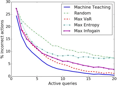
We evaluated three active query strategies from the litera-ture:Max Entropy, a strategy proposed by Lopes et al. (Lopes, Melo, and Montesano 2009) that queries the state with the highest action entropy,Max Infogain, a strategy proposed by Cui at al. (Cui and Niekum 2017) that selects the trajectory with the largest expected change in the posteriorP(R|D), and Max VaR, a recently proposed risk-aware active IRL strategy (Brown, Cui, and Niekum 2018) that utilizes prob-abilistic performance bounds for IRL (Brown and Niekum 2018a) to query for the optimal action at the state where the maximum likelihood action given the current demonstrations has the highest 0.95-Value-at-Risk (95th-percentile policy loss over the posterior) (Jorion 1997). We compare these al-gorithms against random queries and against the maximally informative sequence of queries found using SCOT.
We ran an experiment on 100 random 10x10 grid worlds with 10-dimensional binary features. Figure 2 shows the per-formance loss for each active IRL algorithm. Each iteration corresponds to a single state query and a corresponding opti-mal trajectory from that state. After adding each new trajec-tory toD, the MAP reward function is found using Bayesian IRL (Ramachandran and Amir 2007), and the corresponding optimal policy is compared against the optimal policy under the true reward function.
Avg. number of(s, a)pairs Avg. policy loss Avg. % incorrect actions Avg. time (s)
UVM (105) 5.150 1.539 31.420 567.961
UVM (106) 6.650 1.076 19.568 1620.578
UVM (107) 8.450 0.555 18.642 10291.365
SCOT 17.160 0.001 0.667 0.965
Table 1: Comparison of Uncertainty Volume Minimization (UVM) and Set Cover Optimal Teaching (SCOT) averaged across 20 random 9x9 grid worlds with 8-dimensional features. UVM(x) was run usingxMonte Carlo samples. UVM underestimates the number of(s, a)pairs needed to teachπ∗.
Figure 2: Performance of active IRL algorithms compared to an approximately optimal machine teaching benchmark. Results are averaged over 100 random 10x10 grid worlds.
and Montesano 2009). Max VaR and Max Infogain perform better than Max Entropy for later queries. By benchmarking the against SCOT we see that Max VaR queries are a good approximation of maximally informative queries.
7.2
Using optimal teaching to improve IRL
We next use machine teaching as a novel way to improve IRL when demonstrations are known to be informative. Human teachers are known to give highly informative, non i.i.d. demonstrations when teaching (Ho et al. 2016; Shafto and Goodman 2008). For example, when giving demonstrations, human teachers do not randomly sample from the optimal policy, potentially giving the same (or highly similar) demonstration twice. However, existing IRL ap-proaches usually assume demonstrations are i.i.d. (Ramachan-dran and Amir 2007; Ziebart et al. 2008; Babes et al. 2011; Fu, Luo, and Levine 2017). We propose an algorithm called Bayesian Information-Optimal IRL (BIO-IRL) that adds a no-tion of demonstrator informativeness to Bayesian IRL (BIRL) (Ramachandran and Amir 2007). Our insight is that if a learner knows it is receiving demonstrations from a teacher, then the learner should search for a reward function that makes the demonstrations look both optimal and informative.
BIO-IRL algorithm Our proposed algorithm leverages the assumption of an expert teacher: demonstrations not only fol-lowπ∗, but are also highly informative. We use the following
likelihood for BIO-IRL:
P(D|R)∝Pinfo(D|R)· Y
(s,a)∈D
P((s, a)|R) (23)
whereP((s, a)|R)is the standard BIRL softmax likelihood that computes the probability of taking actionain states
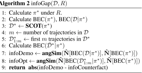
underRandPinfo(D|R)measures how informative the entire demonstration setDappears underR.
We computePinfo(D|R)as follows. Given a demonstra-tion setDand a hypothesis reward functionR, we first com-pute the information gap, infoGap(D, R), which uses behav-ioral equivalence classes to compare the relative informative-ness ofDunderR, with the informativeness of the maximally informative teaching setD∗underR(see Algorithm 2). We estimate informativeness by computing the angular similarity between half-space normal vectors (see (Brown and Niekum 2018b) for details). BIO-IRL uses the absolute difference between angular similarities to counterfactually reason about the gap in informativeness between the actual demonstra-tions and an equally sized set of demonstrademonstra-tions designed to teachR. Given the actual demonstrationDand the machine teaching demonstrationD∗underR, we let
Pinfo(D|R)∝exp(−λ·infoGap(D, R)) (24)
whereλ≥0is a hyperparameter modeling the confidence that the demonstrations are informative. Ifλ= 0, then BIO-IRL is equivalent to standard BBIO-IRL.
The main computational bottlenecks in Algorithm 2 are finding the optimal policy for R∗, and computing the ex-pected feature counts for state-action pairs that are used to calculate the various BEC constraints. Computing the op-timal policy π∗ is already required for BIRL. Computing the expected feature counts for the behavioral equivalence classes is equivalent to performing a policy evaluation step which is computationally cheaper than fully solving forπ∗
(Barreto et al. 2017). By caching BEC(π∗)for each reward function it is possible to save significant computation time during MCMC by reusing the cached BEC if a proposalR
satisfies the vectorized version of Theorem 1 (see (Choi and Kim 2011) and Corollary 2 in (Brown and Niekum 2018b)).
Demonstration
A
B
C
D
Policy Candidates Chain MDP
Figure 3: Simple Markov chain with three features (orange, white, black) and two actions available in each state. Left: a single demonstrated trajectory. Center: all policies that are consistent with the demonstration. Right: likelihoods for BIRL and BIO-IRL withλ= 1 and 10. BIRL gives all rewards that lead to any of the policy candidates a likelihood of 1.0 since it only reasons about the optimality of the demonstration under a hypothesis reward. BIO-IRL reasons about both the optimality of the demonstration and the informativeness of the demonstration and gives highest likelihood to reward functions that induce policy A.
Algorithm 2infoGap(D, R)
1: Calculateπ∗underR.
2: Calculate BEC(π∗), BEC(D|π∗)
3: D∗←SCOT(π∗)
4: m←number of trajectories inD 5: D∗
1:m←firstmtrajectories inD∗ 6: Calculate BEC( ¯D∗|π∗)
7: infoDemo←angSim(Nˆ[BEC(D|π∗)],Nˆ[BEC(π∗)])
8: infoOpt←angSim(Nˆ[BEC(D∗
1:m|π∗)],Nˆ[BEC(π∗)]) 9: return abs(infoDemo - infoCounterfact)
example, if the black feature was always preferred over white and orange, a maximally informative demonstration would have demonstrated a trajectory that started in the leftmost state and moved right until it reached the rightmost state.
Because the likelihood function for standard BIRL only measures how well the demonstration matches the optimal policy for a given reward function, BIRL assigns equal likeli-hoods to all reward functions that result in one of the policy candidates shown in the center of the Figure 3. The bar graph in Figure 3 shows the likelihood of each policy candidate un-der BIRL and BIO-IRL with differentλparameters. Rather than assigning equal likelihoods, BIO-IRL puts higher likeli-hood on Policy A, the policy that makes the demonstration appear both optimal and informative. Changing the likeli-hood function to reflect informative demonstrations results in a tighter posterior distribution, which is beneficial when reasoning about safety in IRL (Brown and Niekum 2018a).
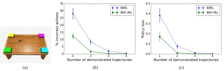
We also evaluated BIO-IRL in a ball sorting task shown in Figure 4(a). In this task, balls start in one of 25 evenly spaced starting conditions and need to be moved into one of four bins located on the corners of the table. Demonstrations are given by selecting an initial state for the ball and moving the ball until it is in one of the bins. Actions are discretized to the four cardinal directions along the table top and the reward is a linear combination of five indicator features representing whether the ball is in one of the four bins or on the table. We generated demonstrations from 50 random rewards with
γ= 0.95. This provides a wide variety of preferences over
bin placement depending on the initial distance of the ball to the different bins. We used SCOT to generate informative demonstrations which were given sequentially to BIRL and BIO-IRL. Figure 4 shows that BIO-IRL is able leverage in-formative, non-i.i.d. demonstrations to learn more efficiently than BIRL (see (Brown and Niekum 2018b) for details).
8
Summary and Future Work
We formalized the problem of optimally teaching an IRL agent as a machine teaching problem and proposed an effi-cient approximation algorithm, SCOT, to solve the machine teaching problem for IRL. Through a set-cover reduction we avoid sampling and use submodularity to achieve an efficient approximation algorithm with theoretical guarantees that the learned reward and policy are correct. Our proposed approach enables an efficient and robust algorithm for selecting maxi-mally informative demonstrations that shows several orders of magnitude improvement in computation time over prior work and scales better to higher-dimensional problems.
For our first application of machine teaching for IRL we ex-amined using SCOT to approximate lower bounds on sample complexity for active IRL algorithms. Benchmarking active IRL against an approximately optimal query strategy shows that a recent risk-sensitive IRL approach (Brown, Cui, and Niekum 2018) is approaching the machine teaching lower bound on sample complexity for grid navigation tasks.
Our second application of machine teaching demonstrated that an agent that knows it is receiving informative demon-strations can learn more efficiently than a standard Bayesian IRL approach. When humans teach each other we typically do not randomly pick examples to show, rather expert teach-ers cherry-pick pick highly informative demonstrations that highlight important details and guide the learner away from common pitfalls. However, most IRL algorithms assume that demonstrations are sampled i.i.d. from the demonstrator’s policy. We proposed BIO-IRL as a way to use machine teach-ing to relax i.i.d. assumptions and correct for demonstration bias when learning from an informative teacher.
(a) (b) (c)
Figure 4: (a) Ball sorting task. The ball starts at one of 36 positions on the table and must be moved into one of four bins depending on the demonstrator’s preferences. 0-1 action losses (b) and policy value losses for MAP policies found by BIO-IRL and BIRL when receiving informative demonstrations. Error bars are 95% confidence intervals around the mean from 50 trials.
continuous (Barreto et al. 2017). Additionally, behavioral equivalence classes can be approximated for continuous state spaces by sampling a representative set of starting states. Given an approximation of the BEC for continuous spaces, SCOT is still guaranteed to terminate and retain efficiency (see (Brown and Niekum 2018b)). Future work also includes using SCOT to approximate the theoretical lower bound on sample complexity for more complicated active learning do-mains, benchmarking other active learning approaches, and using our proposed machine teaching framework to rank com-mon LfD benchmarks according to their inherent teaching difficulty. Future work should also investigate methods for estimating demonstrator informativeness as well as methods to detect and correct for other demonstrator biases in order to learn more efficiently from non-i.i.d. demonstrations.
There are many other interesting possible applications of machine teaching to IRL. One potential application is to use machine teaching to study the robustness of IRL algorithms to poor or malicious demonstrations by studying optimal demonstration set attacks and defenses (Mei and Zhu 2015; Alfeld, Zhu, and Barford 2017). Machine teaching for se-quential decision making tasks also has applications in ad hoc teamwork (Stone et al. 2010) and explainable AI (Gun-ning 2017). In ad hoc teamwork, one or more robots or agents may need to efficiently provide information about their in-tentions without having a reliable or agreed upon commu-nication protocol. Agents could use our proposed machine teaching algorithm to devise maximally informative trajecto-ries to convey intent to other agents. Similarly, in the context of explainable AI, a robot or machine may need to convey its intention or objectives to a human (Huang et al. 2017). Simply showing a few maximally informative examples can be a simple yet powerful way to convey intention.
Acknowledgments
This work has taken place in the Personal Autonomous Robotics Lab (PeARL) at The University of Texas at Austin. PeARL research is supported in part by the NSF (IIS-1724157, IIS-1638107, IIS-1617639, IIS-1749204) and ONR (N00014-18-2243).
References
Alfeld, S.; Zhu, X.; and Barford, P. 2017. Explicit defense actions against test-set attacks. InAAAI, 1274–1280. Argall, B. D.; Chernova, S.; Veloso, M.; and Browning, B. 2009. A survey of robot learning from demonstration. Robotics and Autonomous Systems57(5):469–483.
Arora, S., and Doshi, P. 2018. A survey of inverse rein-forcement learning: Challenges, methods and progress.arXiv preprint arXiv:1806.06877.
Babes, M.; Marivate, V.; Subramanian, K.; and Littman, M. L. 2011. Apprenticeship learning about multiple intentions. In Proceedings of the 28th International Conference on Machine Learning (ICML-11), 897–904.
Balbach, F. J., and Zeugmann, T. 2009. Recent developments in algorithmic teaching. In International Conference on Language and Automata Theory and Applications, 1–18. Barreto, A.; Dabney, W.; Munos, R.; Hunt, J. J.; Schaul, T.; van Hasselt, H. P.; and Silver, D. 2017. Successor features for transfer in reinforcement learning. InAdvances in neural information processing systems, 4055–4065.
Brown, D. S., and Niekum, S. 2018a. Efficient Probabilistic Performance Bounds for Inverse Reinforcement Learning. In AAAI Conference on Artificial Intelligence.
Brown, D. S., and Niekum, S. 2018b. Machine teaching for inverse reinforcement learning: Algorithms and applications. arXiv preprint arXiv:1805.07687(Full paper).
Brown, D. S.; Cui, Y.; and Niekum, S. 2018. Risk-aware active inverse reinforcement learning. InProceedings of the 2nd Annual Conference on Robot Learning (CoRL). Cakmak, M., and Lopes, M. 2012. Algorithmic and human teaching of sequential decision tasks. InAAAI.
Choi, J., and Kim, K.-E. 2011. Map inference for bayesian inverse reinforcement learning. InAdvances in Neural Infor-mation Processing Systems, 1989–1997.
Cui, Y., and Niekum, S. 2017. Active learning from critiques via bayesian inverse reinforcement learning. InRobotics: Science and Systems Workshop on Mathematical Models, Algorithms, and Human-Robot Interaction.
Dayan, P. 1993. Improving generalization for temporal difference learning: The successor representation. Neural Computation5(4):613–624.
Doliwa, T.; Fan, G.; Simon, H. U.; and Zilles, S. 2014. Recur-sive teaching dimension, vc-dimension and sample compres-sion.The Journal of Machine Learning Research15(1):3107– 3131.
Fu, J.; Luo, K.; and Levine, S. 2017. Learning robust re-wards with adversarial inverse reinforcement learning. arXiv preprint arXiv:1710.11248.
Gao, Y.; Peters, J.; Tsourdos, A.; Zhifei, S.; and Meng Joo, E. 2012. A survey of inverse reinforcement learning tech-niques. International Journal of Intelligent Computing and Cybernetics5(3):293–311.
Gao, Z.; Ries, C.; Simon, H. U.; and Zilles, S. 2017. Preference-based teaching. Journal of Machine Learning Research18(31):1–32.
Goldman, S. A., and Kearns, M. J. 1995. On the complex-ity of teaching. Journal of Computer and System Sciences 50(1):20–31.
Gunning, D. 2017. Explainable artificial intelligence (xai). Hadfield-Menell, D.; Russell, S. J.; Abbeel, P.; and Dragan, A. 2016. Cooperative inverse reinforcement learning. In Ad-vances in Neural Information Processing Systems 29. 3909– 3917.
Ho, M. K.; Littman, M.; MacGlashan, J.; Cushman, F.; and Austerweil, J. L. 2016. Showing versus doing: Teaching by demonstration. InAdvances In Neural Information Process-ing Systems, 3027–3035.
Huang, S. H.; Held, D.; Abbeel, P.; and Dragan, A. D. 2017. Enabling robots to communicate their objectives. InRobotics: Science and Systems.
Jorion, P. 1997. Value at risk. McGraw-Hill, New York.
Liu, J., and Zhu, X. 2016. The teaching dimension of linear learners.Journal of Machine Learning Research17(162):1– 25.
Lopes, M.; Melo, F.; and Montesano, L. 2009. Active learn-ing for reward estimation in inverse reinforcement learnlearn-ing. InJoint European Conference on Machine Learning and Knowledge Discovery in Databases, 31–46. Springer.
Mei, S., and Zhu, X. 2015. Using machine teaching to identify optimal training-set attacks on machine learners. In AAAI, 2871–2877.
Neu, G., and Szepesv´ari, C. 2007. Apprenticeship learning using inverse reinforcement learing and gradient methods. In Proc. of 23rd Conference Annual Conference on Uncertainty in Artificial Intelligence, 295–302.
Ng, A. Y., and Russell, S. J. 2000. Algorithms for inverse reinforcement learning. InICML, 663–670.
Paulraj, S., and Sumathi, P. 2010. A comparative study of
redundant constraints identification methods in linear pro-gramming problems.Mathematical Problems in Engineering. Pirotta, M., and Restelli, M. 2016. Inverse reinforcement learning through policy gradient minimization. InAAAI. Ramachandran, D., and Amir, E. 2007. Bayesian inverse rein-forcement learning. InProceedings of the 20th International Joint Conference on Artifical intelligence, 2586–2591. Rathnasabapathy, B.; Doshi, P.; and Gmytrasiewicz, P. 2006. Exact solutions of interactive pomdps using behavioral equiv-alence. InProceedings of the fifth international joint confer-ence on Autonomous agents and multiagent systems, 1025– 1032.
Sadigh, D.; Sastry, S. S.; Seshia, S. A.; and Dragan, A. 2016. Information gathering actions over human internal state. In IEEE/RSJ International Conference on Intelligent Robots and Systems (IROS), 66–73.
Sadigh, D.; Dragan, A. D.; Sastry, S. S.; and Seshia, S. A. 2017. Active preference-based learning of reward functions. InProceedings of Robotics: Science and Systems (RSS). Settles, B. 2012. Active learning. Synthesis Lectures on Artificial Intelligence and Machine Learning6(1):1–114. Shafto, P., and Goodman, N. 2008. Teaching games: Sta-tistical sampling assumptions for learning in pedagogical situations. InProceedings of the 30th annual conference of the Cognitive Science Society, 1632–1637.
Simonovits, M. 2003. How to compute the volume in high dimension? Mathematical programming97(1):337–374. Singla, A.; Bogunovic, I.; Bart´ok, G.; Karbasi, A.; and Krause, A. 2014. Near-optimally teaching the crowd to classify. InICML, 154–162.
Smith, R. L. 1984. Efficient monte carlo procedures for generating points uniformly distributed over bounded regions. Operations Research32(6):1296–1308.
Stone, P.; Kaminka, G. A.; Kraus, S.; Rosenschein, J. S.; et al. 2010. Ad hoc autonomous agent teams: Collaboration without pre-coordination. InAAAI.
Sutton, R. S., and Barto, A. G. 1998.Reinforcement learning: An introduction, volume 1. MIT press Cambridge.
Valiant, L. G. 1979. The complexity of computing the permanent.Theoretical computer science8(2):189–201. Zeng, Y., and Doshi, P. 2012. Exploiting model equivalences for solving interactive dynamic influence diagrams. Journal of Artificial Intelligence Research43:211–255.
Zhang, H.; Parkes, D. C.; and Chen, Y. 2009. Policy teaching through reward function learning. InProceedings of the 10th ACM conference on Electronic commerce, 295–304. ACM. Zhu, X.; Singla, A.; Zilles, S.; and Rafferty, A. N. 2018. An overview of machine teaching. arXiv preprint arXiv:1801.05927.
Zhu, X. 2015. Machine teaching: An inverse problem to machine learning and an approach toward optimal education. InAAAI, 4083–4087.