Spatial Mixture Models with Learnable Deep Priors for Perceptual Grouping

The Thirty-Third AAAI Conference on Artificial Intelligence (AAAI-19)

Spatial Mixture Models with Learnable Deep Priors for Perceptual Grouping

Jinyang Yuan, Bin Li,

Xiangyang Xue

School of Computer Science, Fudan University Fudan-Qiniu Joint Laboratory for Deep Learning Shanghai Institute of Intelligent Electronics & Systems

{yuanjinyang, libin, xyxue_}@fudan.edu.cn

Abstract

Humans perceive the seemingly chaotic world in a structured and compositional way with the prerequisite of being able to segregate conceptual entities from the complex visual scenes. The mechanism of grouping basic visual elements of scenes into conceptual entities is termed as perceptual grouping. In this work, we propose a new type of spatial mixture models with learnable priors for perceptual grouping. Different from existing methods, the proposed method disentangles the rep-resentation of an object into “shape” and “appearance” which are modeled separately by the mixture weights and the condi-tional probability distributions. More specifically, each object in the visual scene is modeled by one mixture component, whose mixture weights and the parameter of the conditional probability distribution are generated by two neural networks, respectively. The mixture weights focus on modeling spatial dependencies (i.e., shape) and the conditional probability dis-tributions deal with intra-object variations (i.e., appearance). In addition, the background is separately modeled as a special component complementary to the foreground objects. Our ex-tensive empirical tests on two perceptual grouping datasets demonstrate that the proposed method outperforms the state-of-the-art methods under most experimental configurations. The learned conceptual entities are generalizable to novel vi-sual scenes and insensitive to the diversity of objects.

Introduction

The ability to perceive complex visual scenes in a structured and compositional way is crucial for humans to understand the seemingly chaotic world (Lake et al. 2017). Finding the underlying mechanisms of grouping basic visual elements is usually termed as the binding (Treisman 1996; Wolfe and Cave 1999), or more specifically, the perceptual group-ing (Grossberg, Mgroup-ingolla, and Ross 1997) problem, and has been studied extensively in the fields of neuroscience, cognitive science and psychology. Designing more human-like AI systems which learn compositional and disentan-gled representations (Bengio, Courville, and Vincent 2013) is desirable, because of their superior expressiveness and generalization ability compared to those systems learning a single complex representation. Complex visual scenes are composed of numerous relatively simpler primitive entities.

∗

Corresponding author

Copyright c2019, Association for the Advancement of Artificial Intelligence (www.aaai.org). All rights reserved.

By hierarchically decomposing the observed visual scenes (Bienenstock, Geman, and Potter 1997), the raw observa-tions can be summarized into organized and compact knowl-edge which is generalizable to an infinite number of novel scenes constructed by the combinations of these primitive entities (Biederman 1987; Hummel and Biederman 1992; van den Hengel et al. 2015).

Inspired by the synchronization theory (Milner 1974), various approaches have been proposed to tackle the per-ceptual grouping problem by using neuronal synchrony as the grouping mechanism (Wang and Terman 1995; Rao et al. 2008; Reichert and Serre 2014). Despite of the satisfac-tory grouping results already obtained, these methods do not learn separate representations for individual objects in the visual scene, which limits the expressiveness and general-ization ability of the learned models. In order to learn disen-tangled and compositional representations of visual scenes, several methods which integrate spatial mixture models with neural networks have been proposed in recent years (Gr-eff, Srivastava, and Schmidhuber 2015; Greff et al. 2016; Pr´emont-Schwarz et al. 2017; Greff, van Steenkiste, and Schmidhuber 2017). In these approaches, different objects are model by different mixture components, and each com-ponent is encouraged to focus on an individual object. The underlying intuition is that the image of visual scene can be decomposed into the pixel-wise weighted sum of recon-structed images of individual objects, with mixture weights computed based on similarities between the images of scene and objects at each pixel.

component due to the diverse combinations of foreground objects.

In this paper, we propose a new type of spatial mix-ture models which places a learnable deep prior of spatial dependencies on mixture weights and considers modeling the background as a special component complementary to the foreground objects. The basic idea is that, in the pro-posed model, the mixture weights should focus on modeling the spatial dependencies (i.e., shapes) of the objects while the conditional probability distributions deal with variations (i.e., appearance) within objects. Instead of modeling mix-ture weights as coefficients with the only constraint that the sum of them equals one at each pixel, they are computed based on the outputs of a neural network with some hidden states as inputs. The inherent structure and learned parame-ters of the network act like priors of spatial dependencies and regularize the model to correctly estimate the shapes of objects in the visual scenes. By constructing the mixture weights in an innovative manner inspired by the truncated stick-breaking process, foreground objects and the back-ground which is harder to represent are modeled differently. Because the background is considered as a special compo-nent whose mixture weights are implicitly determined by es-timations of less varying foreground objects, the proposed method can thus achieve better compositionality and gener-alizes better to novel visual scenes.

We evaluate our method on two perceptual grouping datasets, in which images are composed of simple shapes or handwritten images, under different experimental config-urations. Extensive empirical results suggest that represent-ing the complex regions of background pixels in a compo-sitional manner is crucial to high-quality grouping results. Compared with two state-of-the-art perceptual grouping al-gorithms, the proposed method not only achieves compara-ble or higher grouping accuracies, but also better estimates the images of individual objects from the image of visual scene. By disentangling the representation of an object into “shape” and “appearance” which are modeled separately by the mixture weights and the conditional probability distri-butions, the proposed method can better learn the spatial dependencies of pixels. The learned conceptual entities are generalizable to novel visual scenes and insensitive to the diversity of objects.

Preliminaries

Perceptual Grouping

Perceptual grouping is a type of binding problem that stud-ies how brains arrange elements of visual scenes into con-ceptual entities like objects or patterns. Based on the induc-tive biases that are either innate or learned from experiences, humans tend to segregate, for example, the upper-left cor-ner image in Figure 1a into three white hollow shapes and one black background although these shapes are connected and partially overlapped. The underlying mechanisms have been studied extensively for years. Gestalt psychologists suggested that humans perceive meaningful contents from the sensory information based on inborn mental laws, and summarized their theories into several rule-based principles

of perception (e.g. proximity, similarity, continuity, closure, and common fate) which is often known as Gestalt laws of grouping (Goldstein and Brockmole 2016). The principle of common fate differs from others in that it requires tempo-ral information and is only applicable when relative motions exist. In this work, we only consider utilization of spatial information and focus on building models which follow the principles of proximity, similarity, continuity, and closure by learning prior knowledge of spatial dependencies from data in an unsupervised setting.

Spatial Mixture Model

In spatial mixture models, pixels are assumed to be gener-ated independently from the mixture. Correlations between pixels can be achieved by assuming conditional probabil-ity distributions, or mixture weights, or both of them to be spatially dependent. LetXmbe themth pixel of imageX,

andZmbe the latent variable specifying the mixture

com-ponent ofXm.θk,m={θck,m,θ w

k,m}represents parameters

for generatingXmin thekth component. For the sake of

no-tational simplicity, we letpm,k=P(Xm|Zm=k;θck,m)and

πm,k = P(Zm=k;θw:,m) = θ w

k,m. The log probability of

observing imageXis given by

logP(X;θ) =X

m

logX

k

pm,kπm,k

Computing the maximum likelihood estimate (MLE) of θ directly is difficult due to the existence of unobserved component assignments. Approximated estimates can be ob-tained iteratively by applying the Expectation-Maximization (EM) algorithm. Letγ_m,k(t) denote the posterior probability at thetth iterationP(Zm=k|Xm;θ

(t)

k,m), which is computed by

γ_m,k(t) = p

(t) m,kπ

(t) m,k

P k0p

(t) m,k0π

(t) m,k0

(1)

Parameters are updated usingθ(t+1)= arg max_θQ(θ;θ(t)), whereQ(θ;θ(t))is the Q-function defined as

Q(θ;θ(t)) =X

m X

k

γ(_m,kt) (logpm,k+ logπm,k) (2)

Neural Expectation Maximization

Neural Expectation Maximization (N-EM) (Greff, van Steenkiste, and Schmidhuber 2017) is a state-of-the-art spa-tial mixture model for solving the perceptual grouping prob-lem. In N-EM, both conditional probability distributions and mixture weights are modeled as spatially dependent. Param-etersθc_k,m=fφ(sk)mare generated by a neural networkfφ

with some hidden statessk as inputs, and mixture weights

πm,kare computed based onθc:,m.

Because of the non-linearity of neural networks, the opti-mal hidden states∗

kthat maximizesQ(θ;θ (t)₎

does not have a closed-form solution. Two types of generalized EM algo-rithms were proposed to solve this problem. One is to utilize the gradient descent to optimizeskiteratively

s(_kt+1)=s(_kt)+ηX

m

γ_m,k(t) ∂logpm,k ∂θck,m

∂θc_k,m

∂sk _s

k=s(kt)

Another is to mimic the process of gradient descent by a recurrent neural network (RNN). The neural networkfφ is

trained by the backpropagation through time (BPTT) algo-rithm (Robinson and Fallside 1987; Werbos 1988).

The loss function of each image is given by

L=₋X

m X

k

γm,k(logpm,k+ logπm,k)

+λX

m X

k

(1₋γm,k)DKL(pprior||pm,k) (4)

This loss function consists of two parts. The first part is the negative Q-function which measures the reconstruction er-rors. The second part is the weighted sum of the Kullback-Leibler (KL) divergences between the conditional probabil-ities pm,k and a distributionpprior predefined by the prior

knowledge of the image (e.g. the background intensities).

pm,kis encouraged to be close to the distribution of

back-ground when thekth component is unconfident that themth pixel should be assigned to it (γm,kis small).

Spatial Mixture Model with

Learnable Deep Priors

Except the implicit restriction that the mixture weights at each pixel should sum up to 1(P

kπm,k= 1,∀m), N-EM

does not place any constraint onπm,k. Mixture weights are

assumed to be spatially dependent in N-EM, and the opti-mal weightsπ∗_m,k that maximizes the Q-function is given by π_m,k∗ = γm,k/Pk0γm,k0 = γ_m,k. The ability to dis-tinguish objects with similar intensities relies on spatially dependent conditional probabilities with parameters gener-ated by a neural network. One downside of this approach is the assumption of spatial dependencies for both conditional probabilities and mixture weights, which leads to entan-gled learning of correlations between pixels. This assump-tion also does not fit well with the principle of similarity (elements composing the same object should resemble each other) in the Gestalt laws of grouping. Moreover, the back-ground is not explicitly modeled by a mixture component.

To better follow the principle of similarity and model the background pixels, we integrate neural networks and the EM algorithm in a different way. Instead of modeling correla-tions between pixels by generating spatially dependent pa-rameters of conditional probabilitiespm,kwith a neural

net-workfφ and obtaining the mixture weightsπm,kbased on

the posterior inference results, we apply the neural network

fφto compute spatially dependent mixture weightsπm,kand

an additional networkgψto model spatially independent

pa-rameters ofpm,k. In a sense, the neural networkfφacts like

learnable priors of spatial dependencies in our method. Mix-ture weights are regularized by both the intrinsic strucMix-ture and learnable parameters of the neural network. In the fol-lowing, we first introduce our approach in a general way and then make a concrete example for clarity.

Truncated Stick-Breaking Mixture Weights

The spatially dependent mixture weightsπm,kare computed

based on outputs of a neural networkfφand are constrained

by the structure and parameters of the network. LetKbe the number of components,skthe hidden state vector of thekth

component, andσ(_·)the sigmoid function.ck,mis defined

as σ(fφ(sk)m). The computation ofπm,k which shares a

similar form to the truncated stick-breaking process gives

πm,k=

_c

k,mQk0_<k(1−ck0_,m), k < K

Q

k0_<K(1−ck0_,m), k=K (5)

(5) differs from the truncated stick-breaking process in that the length of stickck,mis computed by a neural network

in-stead of sampled from the beta distribution. Only the first

K₋1 components are assigned with hidden state vectors which describe the shapes of foreground objects. Complex-shaped background regions are estimated based on the pre-dicted shapes of these foreground objects.

Applying the softmax function to the outputs of neural networks is another viable way of modeling probabilities. The main consideration of choosing (5) over the softmax function is compositionality. The purpose of applying the mixture model is to decompose the complex visual scene into simpler components. Generally speaking, objects in the visual scene are relatively easy to represent. The background pixels, however, are almost as hard to model as the visual scene due to the diverse combinations of foreground objects. The softmax function treats each component equally, and

K ₋1 simple and1 complex hidden state vectors are re-quired to generate the mixture weights forK components. When using (5), onlyK₋1hidden state vectors are needed. The complex mixture weights of the background component is determined by these simple states vectors.

Conditional Probabilities

The conditional probabilities pm,k are assumed to be

spa-tially independent in the proposed method. Letθc_kbe the pa-rameters of conditional probabilitiespm,k. If no constraint

is added toθck, the optimal solution that maximizes the

Q-function can be obtained by setting the derivative of (2) with respect toθc_kto zero. To lower the complexity of backprop-agation and stabilize the training of neural networks, values ofθc_kare not updated using the closed-form solution. Allθc_k withk < Kare outputs of a neural networkgψwith hidden

statesskas inputs. ParametersθcKfor the background

com-ponent are modeled as learnable variables that are optimized by gradient descent in the M-step of the EM algorithm.

Optimization of Mixture Model Parameters

Hidden state vectors sk can be updated by either gradient

descent with a learnable learning rate or an RNN which im-itate the behavior of gradient descent. For the sake of no-tational simplicity, outputs of the neural networksfφ(sk)m

andgψ(sk)are denoted byfk,mandgk, respectively. If

us-ing gradient descent as the update rule, hidden statesskwith

1_≤k < Kare updated by

s(_kt+1)=s(_kt)+ηs X

m

γ(_m,kt) ∂logpm,k ∂gk

∂gk

∂sk

+X

k0_≥k

γ_m,k(t) 0

∂logπm,k0

∂fk,m

∂fk,m

∂sk

_s

k=s(kt)

If applying an RNN to learn the procedure of gra-dient descent, inputs to the RNN are features extracted from the concatenation of P

mγ (t)

m,k(∂logpm,k/∂gk) and

allP k0_≥kγ

(t)

m,k0(∂logπm,k0/∂f_k,m)with1 ≤m≤M by an encoder network.

The update rule for the parametersθcKis given by

θc_K(t+1)=θc_K(t)+ηθ X

m

γ_m,K(t) ∂logpm,K ∂θc_K

_θc

K=θcK(t)

(7)

Learning of Neural Networks

Neural networksfφandgψare trained by BPTT algorithm.

The loss function is chosen as

L=₋X

m X

k

γm,k(logpm,k+ logπm,k)

+λX

m

DKL(pprior||pm,K) (8)

As with the loss function (4) used in N-EM, (8) also consists of the Q-function term and a regularization term. This reg-ularization acts like a simplified version of the inductive bi-ases required for human to solve the figure-ground organiza-tion problem (distinguishing a figure from the background). In N-EM, prior information of the backgroundpprioris used

to regularize the conditional probability distributions of all mixture components. In our method, the conditional distri-bution of the background componentpm,Kis encouraged to

be similar topprior, so that the network can better focus on

modeling the foreground objects.

Example: Gaussian Conditional Distribution

The conditional probability distribution of a pixel given its component assignment is usually assumed to be Gaussian for real-valued images, and Bernoulli for binary images. We consider only Gaussian distribution in this section (detailed procedures for each image in an epoch are described in Al-gorithm 1). Formulas for other types of probability distribu-tions can be derived with little modification. Only the means of the Gaussian distributions are learnable parameters, and the variances are assumed to be constant and set toα−1_with

αbeing a hyperparameter tuned by cross-validation. Except for the last component, the means of the Gaussian distribu-tions are computed by the neural networkgψ. For theKth

component, it is modeled as a parameterµK that is learned

by gradient descent. Letxmbe the intensity of themth pixel.

The conditional probabilitypm,kis computed by

pm,k=

G(xm;gψ(sk), α−1), k < K

G(xm;µK, α−1), k=K

(9)

Substituting (9) and (5) into (6), the gradient descent up-date rule for hidden states becomes

s(_kt+1)=s(_kt)+ηs X

m

αγ_m,k(t) (xm−g (t) k )

∂gk

∂sk

+ γ_m,k(t) ₋ X

k0_≥k

γ_m,k(t) 0σ(f

(t) k,m)

∂fk,m

∂sk

_s

k=s(kt)

(10)

Algorithm 1Proposed Method (Gaussian Distribution)

// Initialization:

Draws(0)_k randomly from_N(0, σ_init2 I); µ(0)_{K ←}µprior;

fort_←0toT₋1do // E-Step:

f_k,m(t) _←fφ(s (t) k )m; g

(t)

k ←gψ(s (t) k );

Computep(_m,kt) ,π_m,k(t) andγ_m,k(t) using (9), (5) and (1); // M-Step:

ifusing gradient descentthen Updates(_kt+1)using (10); else

u_←αP mγ

(t)

m,k(xm−g (t) k );

vm←γ (t) m,k−

P k0_≥kγ

(t) m,k0σ(f

(t) k,m);

rin←enc([u, v1, v2, . . . , vM]);

s(_kt+1)_←RNN(rin,s (t) k );

end if

Updateµ(_Kt+1)using (11); // Loss:

ComputeL(t)using (8); end for

// Neural Networks and Learning Rates:

Compute the weighted sum of lossesLsum←PtwtL(t);

Updateφ,ψ,ηsandηθbased onLsum;

If updating sk with an RNN, the encoder network enc

transforms the concatenation ofαP mγ

(t)

m,k(xm−g (t) k )and

γ_m,k(t) ₋P k0_≥kγ

(t) m,k0σ(f

(t)

k,m),1≤m≤M to featuresrinas

the inputs to the RNN.

Substituting (9) into (7) and replacingθc_K withµK, the

learnable parameter for the last component is updated by

µ(_Kt+1)=µ(_Kt)+ηθα X

m

γ_m,K(t) (xm−µ (t)

K) (11)

Related Work

Our method is mostly related to N-EM. Same as N-EM, the update rules for the distributed representations of objects in the visual scene are derived from the EM algorithm. Dif-ferent from N-EM, the foreground objects and background are modeled separately in our method, and spatial dependen-cies of pixels are modeled completely by mixture weights.

Experiments

Datasets Our method is evaluated on two datasets derived from a set of publicly released perceptual grouping datasets provided by (Greff, Srivastava, and Schmidhuber 2015; Greff et al. 2016; Greff, van Steenkiste, and Schmidhuber 2017). We refer to these two datasets as theMulti-Shapes

dataset and the Multi-MNIST dataset. The Multi-Shapes dataset consists of4subsets, which differs from each other in either the image size (20_×20or28_×28) or the number of objects in each image (2,3 or 4). Each subset contains 70,000binary images with simple shapes located at random positions. The Multi-MNIST dataset is composed of3 sets with different degrees of object variations. In each sub-set, there are70,000grayscale 48_×48images which con-tain2handwritten digits. Images in both Multi-Shapes and Multi-MNIST datasets may contain overlapped objects.

Comparison Methods The proposed method is compared with two state-of-the-art perceptual grouping algorithms, namely, N-EM (Greff, van Steenkiste, and Schmidhuber 2017) andTagger(Greff et al. 2016). To assess the effective-ness of computing mixture weights using (5), we substitute it with the softmax function and evaluate this modification (refered as softmax method) on the Multi-Shapes dataset. Neural networks are trained with the Adam optimization al-gorithm (Kingma and Ba 2015) for all approaches. To make a fair comparison, we do not specially design the neural net-worksfφandgψfor the proposed method. The structure of

fφ which generates mixture weights in our method is

iden-tical to the network fφ in N-EM. The extra gψ for

com-puting conditional probabilities is simply a one-layer fully-connected neural network, in which the number of parame-ters is equal to the dimension of hidden states and negligible compared to the total number of network parameters.

Evaluation Metrics We use two metrics to evaluate the grouping results. The first isAdjusted Mutual Information

(AMI), which measures the accuracy of mixture assign-ments. To be consistent with previous work (Greff, Srivas-tava, and Schmidhuber 2015; Greff et al. 2016; Greff, van Steenkiste, and Schmidhuber 2017), AMI scores are not computed in the background and overlapping regions. The second isMean Squared Error(MSE), which computes the smallest mean squared differences between the estimated images of individual objects and the ground truth images over all possible permutations (formulated as the assignment problem and solved efficiently by the Hungarian method). MSE scores are evaluated at all pixels.

Perceptual Grouping Performance Comparisons

Performances of Tagger, N-EM and the proposed method are compared on two subsets of the Multi-Shapes dataset which

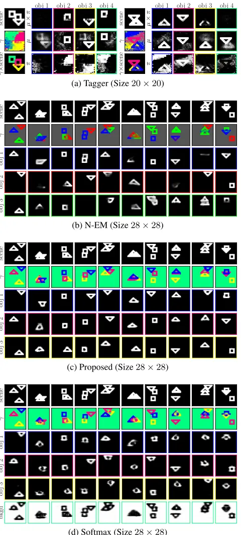
differ from each other in image size (20_×20and28_×28). Images in both subsets contain 3 objects. Because objects in both subsets are of the same size,20_×20images which consist of less pixels are more likely to contain overlapped objects, and performing perceptual grouping on them is not necessarily easier. For Tagger, parameters of mixture models are updated via a3-layer Ladder Network. For N-EM and the proposed method, the encoder and decoder networks are convolutional neural networks (CNNs) with2convolutional, 2fully-connected and3layer normalization (Ba, Kiros, and Hinton 2016) layers. The qualitative results are presented in Figure 1, and the AMI/MSE scores are presented as follows.

Size20_×20 Size28_×28 Tagger 0.933/ 0.71e-2 0.820 / 1.49e-2 N-EM 0.824 / 1.59e-2 0.897 / 0.82e-2 Proposed 0.920 /0.40e-2 0.941/0.28e-2

On the subset consisting of 20 _× 20 images, Tagger achieves the highest grouping accuracy (AMI) and the pro-posed method best estimates the images of individual ob-jects (MSE). The AMI score of the proposed method is slightly lower than Tagger. On the other subset, The pro-posed method achieves both the best AMI and MSE scores. According to Figure 1a (Tagger), the learned knowledge of correlations between pixels are entangled. Both condi-tional probability distributions (row 2; cols 2–5, 7–10) and mixture weights (row 3; cols 2–5, 7–10) contain partial and imperfect information of shape and appearance. It is caused by modeling both conditional probability distributions and mixture weights to be spatially dependent. Another observa-tion is that objects are mainly distinguished based on condi-tional distributions, and the mixture weights assist the seg-regation when ambiguity exists. Although the mixture com-ponent assignments are predicted accurately for foreground objects (row3; cols 1, 6), the background pixels are not well inferred based on posterior probabilitiesγ(row2; cols 1, 6). The possible reason is that the diverse combinations of fore-ground objects prevent backfore-ground pixels from being mod-eled well using non-combinational representations.

In Figure 1b (N-EM), the colors of background pixels in the2nd row are gray (red+green+blue) because the posterior probabilitiesγ are almost identical for all mixture compo-nents. Same as Tagger, background pixels cannot be well de-termined via inferences of posterior probabilities in N-EM. This is caused by a side effect of solving the entangled learn-ing of spatial dependencies by freezlearn-ing the mixture weights during the procedures of expectation maximization. Because correlations between pixels are modeled mainly by condi-tional probability distributions, component assignments are ambiguous in regions where the means of the distributions (rows 3–5) are similar.

scene

obj 1

µ

×

π obj 2 obj 3 obj 4

scene

obj 1

µ

×

π obj 2 obj 3 obj 4

γ µ γ µ

γ

×

scene π

γ

×

scene π

(a) Tagger (Size20×20)

scene

γ

ob

j

1

ob

j

2

ob

j

3

(b) N-EM (Size28×28)

scene

γ

ob

j

1

ob

j

2

ob

j

3

(c) Proposed (Size28×28)

scene

γ

ob

j

1

ob

j

2

ob

j

3

bkgd

(d) Softmax (Size28×28)

Figure 1: Component assignments and reconstructed images of individual objects evaluated on the Multi-Shapes dataset.

Effectiveness of Modeling Background Separately

Besides the observation from Figure 1a that modeling the background as an ordinary component results in imperfect separation of foreground and background based on posterior probabilities, we also assess the effectiveness of modeling

F N N-EM Proposed

AMI MSE AMI MSE

Bernoulli

16 16 0.876 0.95e-2 0.856 1.28e-2 32 16 0.897 0.82e-2 0.868 1.23e-2 32 32 0.816 1.32e-2 0.926 0.43e-2 64 32 0.814 1.34e-2 0.920 0.40e-2 64 64 0.749 1.70e-2 0.941 0.28e-2

Gaussian

16 16 0.687 2.35e-2 0.915 0.68e-2 32 16 0.676 2.34e-2 0.911 0.63e-2 32 32 0.566 2.87e-2 0.914 0.51e-2 64 32 0.503 3.06e-2 0.935 0.30e-2 64 64 0.353 3.77e-2 0.939 0.29e-2

Table 1: Comparisons of AMI and MSE scores under differ-ent choices of conditional probability distributions.FandN

are respective dimensions of RNN inputs and hidden states.

the background separately by evaluating the performances of the softmax method on the second subset (size28_×28) used in the previous experiment. The best AMI and MSE scores achieved are0.875and1.10_×10−2_{, which are}

signifi-cantly worse than the results of the proposed method (0.941 and0.28_×10−2_{). The burden of representing the complex}

background with a single hidden state vector prevents the model to focus on spatial dependencies of foreground pix-els. The qualitative results of the softmax method is shown in Figure 1d. The estimated images of individual objects are not visually plausible although the results of posterior infer-ences (row 2) are satisfactory.

Generalizability and Sensitivity Analyses

Generalizability of Compositional Representations To illustrate the generalizability of the learned compositional representations, the proposed method are evaluated on three subsets of the Multi-Shapes dataset that differ in the number of objects in images. Results of N-EM are also presented. Models of both methods are trainedonlyon the second sub-set. The AMI/MSE scores are shown below.

N-EM Proposed

2 Objects 0.906/ 0.98e-2 0.961/0.11e-2

3 Objects (Train) 0.897 /0.82e-2 0.941 / 0.28e-2 4 Objects 0.838 / 1.44e-2 0.901 / 0.69e-2

For both approaches, the learned representations of concep-tual entities generalize well to visual scenes containing more or less objects. The accuracies of estimated mixture compo-nent assignment are slightly higher when the task is simpler, and moderately lower when dealing with more challenging visual scenes. The MSE score of N-EM becomes slightly worse on the simpler task.

F N N-EM Proposed

AMI MSE AMI MSE

#1

32 16 0.780 1.17e-2 0.748 1.89e-2 32 32 0.573 1.54e-2 0.765 1.64e-2 64 32 0.521 1.54e-2 0.787 1.35e-2 64 64 0.391 1.79e-2 0.790 1.30e-2

#2

32 16 0.317 2.86e-2 0.719 2.07e-2 32 32 0.254 2.75e-2 0.704 2.04e-2 64 32 0.194 2.71e-2 0.719 1.61e-2 64 64 0.152 2.73e-2 0.676 1.63e-2

#3

32 16 0.335 2.93e-2 0.715 2.16e-2 32 32 0.223 3.15e-2 0.702 2.07e-2 64 32 0.185 2.94e-2 0.705 1.69e-2 64 64 0.158 2.84e-2 0.683 1.62e-2

Table 2: AMI and MSE scores evaluated on different sub-sets of the Multi-MNIST dataset. F andN are respective dimensions of RNN inputs and hidden states.

The proposed method, on the other hand, are less sensitive to the form of conditional distributions.

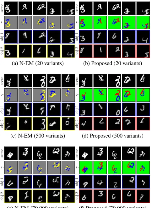
Sensitivity to Diversity of Objects The Multi-MNIST dataset is much more challenging than the Multi-Shapes dataset for the larger image size (48_×48 versus 20_×20 or 28_×28), as well as higher degrees of both inter-object variations (the number of unique objects) and intra-object variations (intensities of pixels belonging to the same ob-ject). There are 3subsets in this dataset. Subsets 1, 2 and 3 are constructed using 20,500 and70,000 unique digits, respectively. Different from the first two subsets, the digits composing images in the test set of subset 3 do not exist in the training and validation set. We evaluate the perfor-mances of N-EM and the proposed method on these subsets, and compare the sensitivities to object diversities of the two approaches. Experimental results are presented in Table 2.

When the diversity of objects is small, N-EM and the proposed method perform similarly well. N-EM achieves slightly higher AMI score and the proposed method attains lower MSE score. As the variations of objects increase, the performance of the proposed method drops moderately, and the grouping results of N-EM decline significantly. On sub-sets 2 and 3, both methods achieve the highest AMI scores when dimensions of RNN inputs and hidden states are small, and the best MSE scores when these dimensions are slighly larger. The possible reason is that the higher dimensions al-low models to focus on more details and help reconstruct sharper individual digits. The large diversities of objects, on the other hand, misguide models to represent parts of dif-ferent objects in the same mixture component and lower the grouping accuracies as the capacities of models increase.

Figure 2 demonstrates the predicted component assign-ments and reconstructed images of individual objects pro-duced by both methods. On subset 1, the results generated by N-EM are slightly more visually plausible. Except for the occluded regions, details of each object are accurately reconstructed. This is because N-EM allows the conditional

scene

γ

ob

j

1

ob

j

2

(a) N-EM (20 variants)

scene

γ

ob

j

1

ob

j

2

(b) Proposed (20 variants)

scene

γ

ob

j

1

ob

j

2

(c) N-EM (500 variants)

scene

γ

ob

j

1

ob

j

2

(d) Proposed (500 variants)

scene

γ

ob

j

1

ob

j

2

(e) N-EM (70,000 variants)

scene

γ

ob

j

1

ob

j

2

(f) Proposed (70,000 variants) Figure 2: Component assignments and reconstructed images of individual objects evaluated on the Multi-MNIST dataset.

probabilities distributions to vary within each object, which helps better reconstruct the intra-object variations of each digit. Both methods can accurately segregate objects from some complex visual scenes like the last two images in Fig-ure 2a and 2b. On subsets 2 and 3, the estimated images of individual objects generated by N-EM are also sharper than the proposed method. However, each component contains pixels of multiple objects. The proposed method models the spatial dependencies of pixels with prior knowledge of mix-ture weights, and utilizes the principle of similarity implied by the spatially independent conditional distributions to as-sist the learning of correlations between pixels. Empirical results suggest that this scheme is less sensitive to the diver-sities of objects in the visual scenes.

Conclusion

separately represented, the proposed method better learns spatial dependencies than existing methods for perceptual grouping. We have demonstrated that the proposed method is insensitive to diversities of objects, and the learned com-positional representations of individual entities generalize well to visual scenes constructed by novel combinations of these entities. Further research in this direction could be integrating hierarchical spatial mixture models with neural networks and solving higher-level tasks like relational infer-ences based on the learned compositional representations.

Acknowledgments

This work was supported in part by National Key R&D Pro-gram of China (No.2017YFC0803700), NSFC under Grant No.61572138 & No.U1611461, and STCSM Projects under Grant No.16JC1420400 & No.18511103104.

References

Ba, J. L.; Kiros, J. R.; and Hinton, G. E. 2016. Layer nor-malization.arXiv preprint arXiv:1607.06450.

Bengio, Y.; Courville, A.; and Vincent, P. 2013. Repre-sentation learning: A review and new perspectives. IEEE Transactions on Pattern Analysis and Machine Intelligence

35(8):1798–1828.

Biederman, I. 1987. Recognition-by-components: A the-ory of human image understanding. Psychological Review

94(2):115.

Bienenstock, E.; Geman, S.; and Potter, D. 1997. Composi-tionality, MDL priors, and object recognition. InAdvances in Neural Information Processing Systems (NIPS), 838–844. Dempster, A. P.; Laird, N. M.; and Rubin, D. B. 1977. Maxi-mum likelihood from incomplete data via the EM algorithm.

Journal of the Royal Statistical Society. Series B (Method-ological)1–38.

Gilmer, J.; Schoenholz, S. S.; Riley, P. F.; Vinyals, O.; and Dahl, G. E. 2017. Neural message passing for quantum chemistry. InInternational Conference on Machine Learn-ing (ICML), 1263–1272.

Goldstein, E. B., and Brockmole, J. 2016. Sensation and perception. Cengage Learning.

Greff, K.; Rasmus, A.; Berglund, M.; Hao, T.; Valpola, H.; and Schmidhuber, J. 2016. Tagger: Deep unsupervised per-ceptual grouping. InAdvances in Neural Information Pro-cessing Systems (NIPS), 4484–4492.

Greff, K.; Srivastava, R. K.; and Schmidhuber, J. 2015. Binding via reconstruction clustering. arXiv preprint arXiv:1511.06418.

Greff, K.; van Steenkiste, S.; and Schmidhuber, J. 2017. Neural expectation maximization. InAdvances in Neural Information Processing Systems (NIPS), 6691–6701. Grossberg, S.; Mingolla, E.; and Ross, W. D. 1997. Visual brain and visual perception: How does the cortex do percep-tual grouping?Trends in Neurosciences20(3):106–111. Hummel, J. E., and Biederman, I. 1992. Dynamic binding in a neural network for shape recognition. Psychological Review99(3):480.

Kingma, D. P., and Ba, J. 2015. Adam: A method for stochastic optimization. In International Conference on Learning Representations (ICLR).

Lake, B. M.; Ullman, T. D.; Tenenbaum, J. B.; and Gersh-man, S. J. 2017. Building machines that learn and think like people.Behavioral and Brain Sciences40.

Milner, P. M. 1974. A model for visual shape recognition.

Psychological review81(6):521.

Pr´emont-Schwarz, I.; Ilin, A.; Hao, T.; Rasmus, A.; Boney, R.; and Valpola, H. 2017. Recurrent ladder networks. In

Advances in Neural Information Processing Systems (NIPS), 6009–6019.

Rao, A. R.; Cecchi, G. A.; Peck, C. C.; and Kozloski, J. R. 2008. Unsupervised segmentation with dynamical units.

IEEE Transactions on Neural Networks19(1):168–182. Rasmus, A.; Berglund, M.; Honkala, M.; Valpola, H.; and Raiko, T. 2015. Semi-supervised learning with ladder net-works. InAdvances in Neural Information Processing Sys-tems (NIPS), 3546–3554.

Reichert, D. P., and Serre, T. 2014. Neuronal synchrony in complex-valued deep networks. InInternational Conference on Learning Representations (ICLR).

Robinson, A., and Fallside, F. 1987. The utility driven dy-namic error propagation network. University of Cambridge Department of Engineering.

Treisman, A. 1996. The binding problem.Current Opinion in Neurobiology6(2):171–178.

van den Hengel, A.; Russell, C.; Dick, A.; Bastian, J.; Poo-ley, D.; Fleming, L.; and Agapito, L. 2015. Part-based mod-elling of compound scenes from images. In Proceedings of the IEEE Conference on Computer Vision and Pattern Recognition (CVPR), 878–886.

van Steenkiste, S.; Chang, M.; Greff, K.; and Schmidhuber, J. 2018. Relational neural expectation maximization: Unsu-pervised discovery of objects and their interactions. In Inter-national Conference on Learning Representations (ICLR). Wang, D., and Terman, D. 1995. Locally excitatory globally inhibitory oscillator networks.IEEE Transactions on Neural Networks6(1):283–286.

Werbos, P. J. 1988. Generalization of backpropagation with application to a recurrent gas market model. Neural Net-works1(4):339–356.

Wolfe, J. M., and Cave, K. R. 1999. The psychophysical evidence for a binding problem in human vision. Neuron