The Thirty-Third AAAI Conference on Artificial Intelligence (AAAI-19)
Learning Logistic Circuits
Yitao Liang, Guy Van den Broeck
Computer Science Department University of California, Los Angeles{yliang, guyvdb}@cs.ucla.edu
Abstract
This paper proposes a new classification model called logistic circuits. On MNIST and Fashion datasets, our learning algo-rithm outperforms neural networks that have an order of mag-nitude more parameters. Yet, logistic circuits have a distinct origin in symbolic AI, forming a discriminative counterpart to probabilistic-logical circuits such as ACs, SPNs, and PSDDs. We show that parameter learning for logistic circuits is con-vex optimization, and that a simple local search algorithm can induce strong model structures from data.
1
Introduction
Circuit representations are a promising synthesis of sym-bolic and statistical methods in AI. They are “deep” layered data structures with statistical parameters, yet they also cap-ture intricate structural knowledge. Recently, many repre-sentations have been proposed for learning tractable proba-bility distributions: arithmetic circuits (Lowd and Domingos 2008), weighted SDD (Bekker et al. 2015), PSDD (Kisa et al. 2014), cutset networks (Rahman, Kothalkar, and Gogate 2014) and sum-product networks (SPNs) (Poon and Domin-gos 2011). Collectively, these approaches achieve the state of the art in discrete density estimation and vastly outper-form classical probabilistic graphical model learners (Gens and Domingos 2013; Rooshenas and Lowd 2014; Adel, Balduzzi, and Ghodsi 2015; Rahman and Gogate 2016; Liang, Bekker, and Van den Broeck 2017). However, we have not observed the same success when deploying circuit representations forclassification or discriminative learning. Probabilistic circuit classifiers significantly lag behind the performance of neural networks (Benenson 2018).
In this paper, we propose a new classification model calledlogistic circuits, which shares many syntactic proper-ties with the representations mentioned earlier. One can view logistic circuits as the discriminative counterpart to proba-bilistic circuits. Owing to their elegant properties, learning the parameters of a logistic circuit can be reduced to a lo-gistic regression problem and is therefore convex. Learning logistic circuit structure is reduced to a simple local search problem using primitives from the probabilistic circuit learn-ing literature (Liang, Bekker, and Van den Broeck 2017).
Copyright c2019, Association for the Advancement of Artificial Intelligence (www.aaai.org). All rights reserved.
We run experiments on standard image classification benchmarks (MNIST and Fashion) and achieve accuracy higher than much larger MLPs and even CNNs with an or-der of magnitude more parameters. For example, logistic cir-cuits obtain 99.4% accuracy on MNIST. Compared to other tractable learners on MNIST, and the state-of-the-art dis-criminative SPN learner in particular (Peharz et al. 2018), our logistic circuit learner cuts the error rate by a factor of three. Furthermore, we show our learner is highly data effi-cient, managing to still learn well with limited data.
This paper proceeds as follows. Section 2 introduces the syntax and semantics of logistic circuits. Sections 3 and 4 describe our parameter and structure learning algorithms, which Section 5 evaluates empirically. Section 6 elaborates on the connection with tractable generative models, after which we conclude with related and future work.
2
Representation
This section introduces the logistic circuit representation. Notation We use uppercaseX to denote a Boolean ran-dom variable and lowercasexfor a specific assignment to it. Interchangeably, we also interpret Boolean random variables as logical variables. A set of variablesXand their joint as-signmentsxare denoted in bold. A complete assignmentx
to all variables is a possible world, or interchangeably, a data sample. Literals are variablesXor their negation¬X. Log-ical sentences are constructed from literals and connectives such as AND and OR in the standard way. An assignmentx
that satisfies a logical sentenceαis denoted asx|=α.
2.1
Logical Circuits
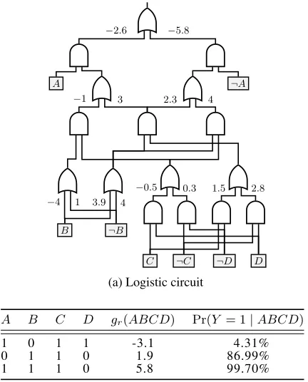
A logical circuit is a directed acyclic graph representing a logical sentence, as depicted in Figure 1a (ignoring parame-ters for now). Each inner node is either an AND gate or an OR gate.1 A leaf (input) node represents a Boolean literal, that is,X or¬X, where the node can only be satisfied ifX
is set to 1 (true) respectively 0 (false).
The following properties are key for logical circuits to be well-behaved (Darwiche and Marquis 2002). An AND gate
1
−2.6 −5.8
−1 3 2.3 4
−0.5 0.3 1.5 2.8
−4 1 3.9 4
A ¬A
B ¬B
C ¬C ¬D D
(a) Logistic circuit
A B C D gr(ABCD) Pr(Y = 1|ABCD)
1 0 1 1 -3.1 4.31%
0 1 1 0 1.9 86.99%
1 1 1 0 5.8 99.70%
(b) Weights and classification probabilities for select examples
Figure 1: A logistic circuit with example classifications.
isdecomposableif its inputs depend on disjoint sets of vari-ables. For example, the top-most AND gates in Figure 1a de-pend onAin their one input and on{B, C, D}in their other input. When an AND gate has two inputs, they are called its prime (left) and sub (right). An OR gate isdeterministicif for any single complete assignment, at most one of its inputs can be set to1. For example, the left input to the root OR gate in Figure 1a is1precisely whenA = 1, and its other input is1precisely whenA= 0.
Logical circuits can be extended toprobabilistic circuits
that represents a probability distribution over binary random variables, for example by parameterizing wires with condi-tional distributions (Kisa et al. 2014). Probabilistic circuits have been successfully used for generative learning (Liang, Bekker, and Van den Broeck 2017). Section 6 will discuss probabilistic circuits in more detail.
2.2
Logistic Circuits
This paper proposeslogistic circuitsfor classification. Syn-tactically, they are logical circuits where every AND is decomposable and every OR is deterministic. However, logistic circuits further associate real-valued parameters
θ1, . . . , θmwith theminput wires to every OR gate. For ex-ample, the root OR node in Figure 1a associates parameters −2.6and−5.8with its two inputs.
To give semantics to logistic circuits, we first characterize how a particular complete assignmentx(one data example) propagates through the circuit.
Definition 1(Boolean Circuit Flow). Consider a determin-istic OR gaten. The Boolean flowf(n,x, c)of a complete assignmentxbetween parentnand childcis
f(n,x, c) =
1 if x|=c 0 otherwise
For example, under the assignmentA= 0,B= 1,C= 1,
D= 0, the root node in Figure 1a has a Boolean circuit flow of 0 with its left child and 1 with its right child. Note that the determinism property guarantees that under every OR gate, for a given examplex, at most one wire has a flow of 1, and the rest has a flow of0.
We are now ready to define the logistic circuit semantics. Definition 2(Logistic Circuit Semantics). A logistic circuit nodendefines the following weight functiongn(x).
– Ifnis a leaf (input) node, thengn(x) = 0.
– Ifnis an AND gate with childrenc1, . . . , cm, then
gn(x) = m
X
i=1 gci(x).
– Ifnis an OR gate with (child node, wire parameter) inputs
(c1, θ1), . . . ,(cm, θm), then
gn(x) = m
X
i=1
f(n,x, ci)·(gci(x) +θi).
At root noderwith weight functiongr(x), the logistic circuit
defines the posterior distribution on class variableY as
Pr(Y = 1|x) = 1
1 + exp (−gr(x))
. (1)
Using Boolean circuit flow, this definition essentially col-lects all the parameters on wires with flow 1 that reach the root, in order to then make a prediction. This is illustrated in Figure 1a by coloring red the gates and wires whose pa-rameters and weight function are propagated upward for the example assignmentA= 0,B= 1,C= 1,D= 0. The lo-gistic circuit in Figure 1a defines the same posterior predic-tions as the table in Figure 1b. Specifically, for the example assignment, the weight function simply sums the parameters colored in red:−5.8 + 2.3 + 3.9 + 1.5 = 1.9. We then apply the logistic function (Eq. 1) to get the classification proba-bilityPr(Y = 1|x) = 1+exp(1−1.9)= 86.99%.
2.3
Real-Valued Data
The semantics given so far assume Boolean inputsx, which is a rather restrictive assumption and prohibits many ma-chine learning applications. Next, we augment the logistic circuit semantics such that they can classify examples with continuous variables.
We interpret real-valued variables q ∈ [0,1]as param-eterizing an (independent) Bernoulli distribution (cf. Xu et al. (2018)). Each continuous variable represents the proba-bility of the corresponding Boolean random variableX. For example, withqsettingA = 0.4,B = 0.8,C = 0.2, and
Definition 3(Probabilistic Circuit Flow). Consider a deter-ministic OR gaten. Letqbe a vector of probabilities, one for each variable inX. The probabilistic flowf(n,q, c)of vectorqbetween parentnand childcis
f(n,q, c) = Prq(c|n) =
Prq(c∧n) Prq(n)
= Prq(c) Prq(n) ,
wherePrq(.)is the fully-factorized distribution where each variable inXhas the probability assigned byq.
Logistic circuit semantics now support continuous data (after normalizing to [0,1]), simply by replacing Boolean flow with probabilistic flow in Definition 2. Note that proba-bilistic circuit flow has Boolean circuit flow as a special case, whenqhappens to be binary. Furthermore, due to the deter-minism and decomposability properties, the probabilities in Definition 3 can be computed efficiently, together with all probabilistic circuit flows and weight functions in the logis-tic circuit. We defer the discussion of these computational details to Section 3.4. In the rest of this paper, we will abuse notation and havexrefer to Boolean inputs as well as con-tinuous inputsqinterchangeably.
3
Parameter Learning
A natural next question is how to learn logistic circuit pa-rameters from complete data, for a fixed given circuit struc-ture (strucstruc-ture learning is discussed in Section 4). Further-more, we ask whether those learned parameters are guaran-teed to be optimal, globally minimizing a loss function. We address these questions by showing how parameter learning can be reduced to logistic regression on a modified set of features, owing to logistic circuits’ strong properties.
3.1
Special Cases
Before presenting the general reduction, we briefly discuss two special cases that establish some intuition.
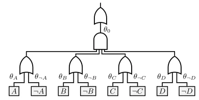
Linear Weight Functions Consider a vanilla logistic re-gression model on input variables (features)X. Does there exist an equivalent logistic circuit with the same weight function? For samplex, logistic regression with parameters θwould have weight functionx·θ. Following Definition 2, we obtain such a simple weight function (linear in the input variables) by placing OR gates over complementary pairs of literals and associating aθparameter which each wire (see Figure 2).2A large parent AND gate collects these variable-wise weights into a single linear sum. Finally, an OR gate at the root adds the bias term regardless of the input.
Proposition 1. For each classical logistic regression model, there exists an equivalent logistic circuit model.
Boolean Flow Indicators Next, let us consider a special case that makes no assumptions about circuit structure, but that requires the inputs to be fully binary. Such a circuit would have Boolean flows through every wire. Instead of
2
The negated variable inputs and parameters θ¬X are
redun-dant, but we keep them for the sake of consistency. Alternatively, we can fixθ¬X= 0for allXto remove this redundancy.
θ0
θA θ¬A θB θ¬B θC θ¬C θD θ¬D
A ¬A B ¬B C ¬C D ¬D
Figure 2: Logistic regression represented as a logistic circuit
working with the input variablesX, we can introduce new features that are indicator variables, telling us how the exam-ple propagates through the circuit, and which wires have a Boolean flow that reaches the circuit root. The circuit flows (indicators) decide which parameters are summed into the weight function; this process has been implicitly revealed in Figure 1a. By introducing such indicators, we can always obtain a linear weight function of composite features that are extracted from samplex. Next, we generalize this idea of introducing wire features to arbitrary logistic circuits.
3.2
Reduction to Logistic Regression
We will now consider the most general case, with continuous input data and no assumptions on the circuit structure. Proposition 2. Any logistic circuit model can be reduced to a logistic regression model over a particular feature set.
Corollary 3. Logistic circuit cross-entropy loss is convex.
To prove Proposition 2, we need to rewrite the classifica-tion distribuclassifica-tion in Definiclassifica-tion 2 as follows.
Pr(Y = 1|x) = 1
1 + exp(−x·θ).
Here,xis some vector of features extracted from the raw examplex. This feature vector can only depend onx; not on the parametersθ. Thus, the fundamental question is whether we can decomposegn(x)intox·θfor all nodesn. We prove this to be true by induction:
– Base case:nis a leaf (input) node. It is obviousgncan be expressed asx·θsincegnalways equals 0.
– Induction step: assumeg of all the nodes under noden
can be expressed asx·θ. We need to consider two cases: 1. If n is an AND gate having (w.l.o.g.) two children, primepand subs. Givengp=xp·θpandgs=xs·θs,
gn=xp·θp+xs·θs
=
xp
xs
·
θp
θs
.
inputs{(c1, θ1), . . . ,(cm, θm)}. Givengci=xci·θci,
gn =
X
i
f(n,x, ci)·(xci·θci+θi)
=
f(n,x, c1)·xc1 f(n,x, c1)
.. .
f(n,x, cm)·xcm
f(n,x, cm)
·
θc1 θ1
.. .
θcm
θm
.
Note that this proof holds true regardless of whether the input samplexis binary or real-valued. With this proof, it is obvious that learning the parameters of a logistic circuit is equivalent to logistic regression on features x. We refer readers to Rennie (2005) for a detailed proof that logistic regression is convex.
Given this correspondence, any convex optimization tech-nique can now be brought to bear on the problem of learn-ing the parameters of a logistic circuit. In particular, we use stochastic gradient descent for this task.
3.3
Global Circuit Flow Features
In the proof of Proposition 2, featuresx are computed re-cursively by induction. However, it is not clear what these features represent, and how they are connected to the input data. In this section we assign semantics to those extracted features. They are theglobal circuit flowof the observed ex-ample through the circuit. Global circuit flow is defined with respect to the root of a logistic circuit.
Definition 4(Global Circuit Flow). Consider a logistic cir-cuit over variablesXrooted at OR gater. The global cir-cuit flowfr(n,x, c)of inputxbetween parentnand child
c is defined inductively as follows. The global circuit flow between rootrand its childcis the (local) probabilistic cir-cuit flow:fr(r,x, c) =f(r,x, c). Then, for any nodenwith
parentsv1, . . . , vm, we have that
– ifnis an AND gate, global flow from childcis
fr(n,x, c) = m
X
i=1
fr(vi,x, n),
– ifnis an OR gate, global flow from childcis
fr(n,x, c) =f(n,x, c)· m
X
i=1
fr(vi,x, n).
The red wires in Figure 1a have a global circuit flow of 1 for the given Boolean input. In general, global circuit flow assigns a continuous probability value to each wire.
Based on global circuit flow, we postulate the following alternative semantics for logistic circuits.
Definition 5(Logistic Circuit Alternative Semantics). Let
Wbe the set of all wires(n, θ, c)between OR gatesnand childrencwith parametersθ. Then, a logistic circuit rooted at noderdefines the weight function
gr(x) =
X
(n,θ,c)∈W
fr(n,x, c)·θ.
Note that the definition of global circuit flows, as well as our alternative semantics, follow a top-down induction. In contrasts, the original semantics in Definition 2 follow a bottom-up induction. We resolve this discrepancy next. Proposition 4. The featuresx constructed in the proof of Proposition 2 are equivalent to global flowsfr(n,x, c). Corollary 5. The bottom-up semantics of Definition 2 and the top-down semantics of Definition 5 are equivalent.
We defer the proof of this proposition to Appendix A. Recall that without parameters, a logistic circuit is sim-ply a logical circuit, which means that gates in a logistic cir-cuit have real meaning: they correspond to some logical sen-tence. Hence, the values of global circuit flow featuresx cor-respond to probabilities of these logical sentences according to the input vectorx. This provides us with a precious oppor-tunity to assign meaning to the features learned by logistic circuits. We will revisit this point in Section 5.4, where we also visualize some global circuit flow features.
3.4
Computing Global Flow Features Efficiently
While logistic circuit parameter learning is convex, we would like to also guarantee that the required feature compu-tation is tractable. This section discusses efficient methods to calculate global flow featuresx(i.e.,fr(n,x, c)) from train-ing samplesxoffline, before parameter learning.
As is clear from Definition 3, circuit flows make exten-sive use of node probabilities. We design our computation to consist of two parts, and dedicate the first part to the calcula-tion of node probabilities. The first part is a bottom-up linear pass over the circuit starting with leaf nodes whose proba-bilities are directly provided by the input sample; see the details in Appendix B. The second part makes use of these node probabilities to calculate the global circuit flow fea-tures in linear time. It is a top-down implementation of the recursion in Definition 4; see its details in Appendix C. Note that these computations correspond to the partial derivative computations used in arithmetic circuits for the purpose of probabilistic inference (Darwiche 2003).
Our algorithm is completely compatible with fast vector arithmetic: instead of inputting one single sample each time, one can directly supply the algorithms with a vector of sam-ples (e.g., a mini batch), and this yields significant speedups.
4
Structure Learning
This section presents an algorithm to learn a compact logical circuit structure for logistic circuits from data. For simplicity of designing the primitive operations, we assume AND gates always have two inputs (prime and sub).
4.1
Learning Primitive
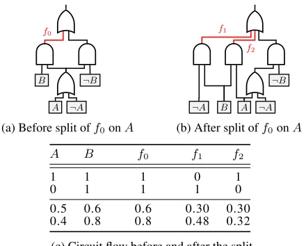
The split operation was first introduced to modify the struc-ture of PSDD circuits (Liang, Bekker, and Van den Broeck 2017). We adopt it here with minor changes3 as the prim-itive operation for our structure learning algorithm.
Split-3
f0
A ¬A
B ¬B
(a) Before split off0onA
f1
f2
A ¬A
¬A B
¬B
(b) After split off0onA
A B f0 f1 f2
1 1 1 0 1
0 1 1 1 0
0.5 0.6 0.6 0.30 0.30 0.4 0.8 0.8 0.48 0.32
(c) Circuit flow before and after the split.
Figure 3: A split changes the circuit flow.
ting an AND gate happens by imposing two additional con-straints that aremutually exclusiveandexhaustive, in partic-ular by making two opposing variable assignments. Execut-ing a split creates partial copies of the gate and some of its decedents. Furthermore, one can choose to duplicate addi-tional nodes up to a fixed depth (3 in our experiments). We refer readers to Liang, Bekker, and Van den Broeck (2017) for further details on the algorithm for executing splits.
Splits are ideal primitives to change the classifier induced by a logistic circuit: they directly affect the circuit flows (see Figure 3). By imposing constraints on AND gates, splits al-ter the node probabilities associated with the affected AND gates. Following Definition 3, the circuit flows on the wires out of those AND gates adapt accordingly. While Figure 3 focuses on the immediately affected wires, the effect of a split on circuit flows can propagate downward for several levels, depending on the depth of node duplication. Still the effects of a split on both the structure of a logistic circuit and the circuit flows are very local and contained in the sub-circuit rooted at the OR parent of the split AND gate. How-ever, its effect on the parameters is global. Once a split is executed, the whole parameter set needs to be re-trained.
4.2
Learning Algorithm
The overall structure learning algorithm for logistic circuits, built on top of the split operation, proceeds as follows. Itera-tively, one split is executed to change the structure, followed by parameter learning. We only consider single-variable split constraints and first select which AND gate to split, followed by a selection of which variable to split on.
When using gradient descent, one hopes that the param-eter on the AND gate output consistently has its partial derivatives pointing in the same direction for all training examples. This will steadily push the parameter to a large magnitude.
If this is not the case, we will use splits to alter the flow of examples through the circuit. Specifically, those AND gates whose associated output parameter has a large variance of its
Table 1: Classification accuracy of logistic circuits in context with commonly used existing models. We report the details of those existing models in Appendix E.
ACCURACY%ONDATASET MNIST FASHION
BASELINE: LOGISTICREGRESSION 85.3 79.3
BASELINE: KERNELLOGISTICREGRESSION 97.7 88.3
RANDOMFOREST 97.3 81.6
3-LAYERMLP 97.5 84.8
RAT-SPN (PEHARZ ET AL. 2018) 98.1 89.5
SVMWITHRBF KERNEL 98.5 87.8
5-LAYERMLP 99.3 89.8
LOGISTICCIRCUIT(BINARY) 97.4 87.6
LOGISTICCIRCUIT(REAL-VALUED) 99.4 91.3
CNNWITH3CONV LAYERS 99.1 90.7
RESNET(HE ET AL. 2016) 99.5 93.6
Table 2: Number of parameters of logistic circuits in con-text with existing SGD-based models, when achieving the classification accuracy reported in Table 1
NUMBER OFPARAMETERS MNIST FASHION
BASELINE: LOGISTICREGRESSION <1K <1K
BASELINE: KERNELLOGISTICREGRESSION 1,521 K 3,930K
LOGISTICCIRCUIT(REAL-VALUED) 182K 467K
LOGISTICCIRCUIT(BINARY) 268K 614K
3-LAYERMLP 1,411K 1,411K
RAT-SPN (PEHARZ ET AL. 2018) 8,500K 650K
CNNWITH3CONV LAYERS 2,196K 2,196K
5-LAYERMLP 2,411K 2,411K
RESNET(HE ET AL. 2016) 4,838K 4,838K
partial derivative (that is, the derivative of the loss function w.r.t. that parameter) requires splitting for the parameters to improve. We simply select the AND gate whose output pa-rameter has the highest training variance.
Given an AND gate to split, we consider candidate vari-ablesX to execute the split with. We construct two sets of training examples that affect this node: in one group, each example is weighted by the marginal probability of X; in the other, with the marginal probability of ¬X. Next, we calculate the within-group weighted variances of the partial derivatives. The variable with the smallest weighted vari-ances gets picked, as this suggests the split will introduce new parameters with gradients that align in one direction.
5
Empirical Evaluation
In this section, we empirically evaluate the competitive-ness of our learner on three aspects: classification accuracy, model complexity, and data efficiency.4 Moreover, we vi-sualize the most important active feature with regards to the given sample to provide local interpretation for why the learned logistic circuit makes such classification.
4
Table 3: Comparison of logistic circuits with MLPs when trained with different percentages of the dataset.
ACCURACY%WITH%OFTRAININGDATA MNIST FASHION
100% 10% 2% 100% 10% 2%
5-LAYERMLP 99.3 98.2 94.3 89.8 86.5 80.9
CNNWITH3 CONVLAYERS 99.1 98.1 95.3 90.7 87.6 83.8
LOGISTICCIRCUIT(BINARY) 97.4 96.9 94.1 87.6 86.7 83.2
LOGISTICCIRCUIT(REAL-VALUED) 99.4 97.8 96.1 91.3 87.8 86.0
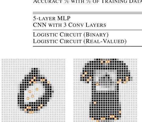
Figure 4: Visualization of the single compositional feature that contributes most to the classification probability with regards to the input image. Features are marked in orange. Left: a digit 0 from MNIST. Right: a t-shirt from Fashion.
5.1
Setup & Data Preprocessing
We choose MNIST and Fashion5as our testbeds. Since lo-gistic circuits are intended for binary classification, we use the standard “one vs. rest” approach to construct an ensem-ble multi-class classifier such that our method can be evalu-ated on these two datasets. When running the binary logistic circuit, we transform pixels that are smaller than their mean plus0.05 standard deviation to 0 and the rest to 1. When running the real-valued version, we transform pixels to[0,1] by dividing them by 255. All experiments start with a pre-defined initial structure; we defer its details to Appendix D. The learned structure with the highest F1 score on validation after 48 hours of running is used for evaluation. All experi-ments are run on single CPUs.
5.2
Classification Accuracy
Table 1 summarizes the classification accuracy on test data. Learning a logistic circuit on the binary data is on par with a 3-layer MLP; the real-valued version outperforms 5-layer MLPs and even CNNs with 3 convolutional layers. The fact that logistic circuits achieve better accuracy than CNNs is surprising, since logistic circuits do not use convolutions, which are specifically designed to exploit image invariances. In addition, we would like to emphasis our comparison with two of the baselines. As parameter learning of logis-tic circuits is equivalent to logislogis-tic regression, one can view structure learning of logistic circuits as a process of con-structing composite features from raw samples. The
signifi-5
A dataset of Zalando’s images, intended as a more challenging drop-in replacement of MNIST (Xiao, Rasul, and Vollgraf 2017).
cant improvement over standard logistic regression demon-strates the effectiveness of our method in extracting valuable features; using kernel logistic regression can only partially bridge the gap in performance, yet as shown later, it does so at the cost of introducing many more parameters.
We also want to call attention to our comparison with RAT-SPN, the current state of the art in discriminative learn-ing for probabilistic circuits. SPN is another form of cir-cuit representation, with less restrictive structure. Parameter learning in SPN is not convex and generally requires other techniques such as EM or non-convex optimization. The em-pirical observation that our method achieves significantly better classification accuracy than RAT-SPN demonstrates that in structure learning, imposing more restrictions on the model’s structural syntax may be beneficial. The syntactic restriction of logistic circuits requires decomposability and determinism; without them, convex parameter learning does not appear to be possible. As structure learning is built on top of parameter learning, a well-behaved parameter learn-ing loss with a unique optimum can provide more informa-tive guidance about how to adapt the structure, leading to a more competitive structure learning algorithm overall.
5.3
Model Complexity & Data Efficiency
Table 2 summarizes the size of all compared models when achieving the reported accuracy. We can conclude that lo-gistic circuits are significantly smaller than the alternatives, despite attaining higher accuracy.
0.6 0.4
0.9 0.1
0.2 0.8 0.6 0.4
0.1 0.9 0.3 0.7 0.1 0.9 0.8 0.2
0.4 0.6
0.2 0.8 0.7 0.3
0.8 0.2 0.5 0.5 0.6 0.4 0.9 0.1
Y ¬Y
A ¬A
B ¬B
C ¬C ¬D D
A ¬A
B ¬B
C ¬C ¬D D
(a) Probabilistic circuit for joint distributionPr(Y, A, B, C, D)
ln0.6 0.4
ln0.9 0.4 ln
0.1 0.6
ln0.2 0.2 ln
0.8
0.8 ln
0.4 0.3
ln0.6 0.7
ln0.1 0.8 ln
0.9 0.2 ln
0.3 0.5 ln
0.7 0.5
ln0.1 0.6 ln
0.9 0.4
ln0.8 0.9
ln0.2 0.1
A ¬A
B ¬B
C ¬C ¬D D
(b) Logistic circuit forPr(Y = 1|A, B, C, D)
Figure 5: A probabilistic circuit with parallel structures under class variableY and its equivalent logistic circuit for predictingY
proposed structure learning algorithm is.
Except on MNIST with10%training samples, real-valued logistic circuits achieve the best classification accuracy. From a top-down perspective, each OR gate of a logistic cir-cuit presents a weighted choice between its wires. Hence, one can view a logistic circuit as a decision diagram. Un-der this perspective, splits refine OR gates’ branching rules. As each branching rule naturally applies to multiple sam-ples, we hypothesize that the splits selected by our structure learning algorithm reflect the general conditional feature in-formation present in the dataset.
5.4
Local Explanation
Next, we aim to share some insights about how to explain the learned logistic circuit. Specifically, we investigate the ques-tion: “Why does the logistic circuit classify a given samplex
asy?” Since any logistic circuit can be reduced to a logistic regression classifier, we can easily find the active global flow feature that contributes most to the given sample’s classifi-cation probability. That is, the feature that maximizesx·θ. We visualize one such feature for MNIST data and one for Fashion in Figure 4 by marking the variables used in the their corresponding logical sentences.
6
Connection to Probabilistic Circuits
In recent years, a large number of tractable probabilis-tic models have been proposed as a target representation for generative learning of a joint probability distribution: arithmetic circuits (Lowd and Domingos 2008), weighted SDD (Bekker et al. 2015), PSDD (Kisa et al. 2014), cutset networks (Rahman, Kothalkar, and Gogate 2014) and sum-product networks (SPNs) (Poon and Domingos 2011). These representations have various syntactic properties. Some put probabilities on terminals, others on edges. Some use logical notation (AND, OR), others use arithmetic notation (×,+). Nevertheless, they are all circuit languages built around theproperties of decomposability and/or determinism.
For our purpose, we consider a simple probabilistic circuit language based on the logistic circuit syntax, where now the
θparameters are assumed to be normalized probabilities.6 Definition 6 (Probabilistic Circuit Semantics). A proba-bilistic circuit nodendefines the following joint distribution. – Ifnis a leaf (input) node, thenPrn(x) = [x|=n].
– Ifnis an AND gate with childrenc1, . . . , cm, then
Prn(x) = m
Y
i=1
Prci(x).
– Ifnis an OR gate with (child node, wire parameter) inputs
(c1, θ1), . . . ,(cm, θm), then
Prn(x) = m
X
i=1
Prci(x)·θi.
Figure 5a shows a probabilistic circuit for the joint dis-tributionPr(Y, A, B, C, D). This tractable circuit language is a relaxation of PSDDs (Kisa et al. 2014) and a specific type of SPN (Poon and Domingos 2011) where determinism holds throughout. It is also a type of arithmetic circuit.
We are now ready to connect logistic and probabilistic cir-cuits. It is well known that logistic regression is the discrim-inative counterpart of a naive Bayes generative model (Ng and Jordan 2002). A similar correspondence holds between our logistic and probabilistic circuits.
Proposition 6. Consider a probabilistic circuit whose struc-ture is of the form(Y∧α)∨(¬Y∧β), where sub-circuitsα andβare structurally identical. Then, there exists an equiv-alent logistic circuit for the conditional probability ofY in the probabilistic circuit. Moreover, this logistic circuit has structure∨αand its parameters can be computed in closed form as log-ratios of probabilistic circuit probabilities.
6
We first depict this correspondence intuitively in Figure 5. The logistic circuit has the same structure as the two halves of the probabilistic circuit, and its parameters are computed from the probabilistic circuit probabilities. The distributions Pr(Y = 1|A, B, C, D)represented by the circuits in Fig-ures 5a and 5b are identical.
Formal Correspondence Next, we present the formal proof of this correspondence for binaryx. Recall that in our circuits, only the input wires of OR gates are parameterized. LetWδ be the set that contains all these wires in circuitδ:
Wδ ={(n, c)|cis a gate with parent OR gaten}.
After expanding the equations in Definition 6 and following the top-down definition of global circuit flow (i.e., following Definition 4), one finds that the joint distribution induced by a probabilistic circuitδcan be rewritten as
Prδ(x) =
Y
(n,c)∈Wδ
fδ(n,x, c)·θδ(n,c).
We will exploit this finding in the derivation of the condi-tional distribution induced by the probabilistic circuitγ = (Y ∧α)∨(¬Y ∧β).
Prγ(Y = 1|x)
= Prγ(Y= 1) Prα(x)
Prγ(Y= 0) Prβ(x) + Pr(Y= 1) Prα(x)
= 1
1 + Prγ(Y=0) Prβ(x)
Prγ(Y=1) Prα(x)
= 1
1 + Prγ(Y=0)
Q
(n,c)∈Wβfβ(n,x,c)θβ(n,c)
Prγ(Y=1)Q(n,c)∈Wαfα(n,x,c)θ α
(n,c)
As stated in Proposition 6 and shown in Figure 5, sub-circuitsαandβshare the same structure. Therefore, we can further simplify this equation as follows.
Prγ(Y = 1|x)
= 1
1 + Prγ(Y=0)
Prγ(Y=1)
Q
(n,c)∈Wαf∨α(n,x, c) θβ(n,c) θα
(n,c)
= 1
1 + exp [−g(x))]= Pr∨α(Y = 1|x) where
g(x) = logPrγ(Y= 1) Prγ(Y= 0)
+ X
(n,c)∈Wα
f∨α(n,x, c) log
θα
(n,c) θ(βn,c)
(2) =θroot∨α +
X
(n,c)∈Wα
f∨α(n,x, c)·θ∨(n,cα). (3)
The transformation from Equation 2 to 3 expresses the logis-tic circuit parameters as the log-ratios of probabilislogis-tic circuit probabilities. For example, the class priors captured in the output wires ofαandβare now combined as a log-ratio to form the bias term for∨α, expressed by the root parameter.
This proof also provides us with a new perspective to un-derstand the semantics of the learned parameters. The pa-rameters represent the log-odds ratio of the features given different classes. Note that by Bayes’ theorem, a naive Bayes model would derive its induced distribution in a sequence of steps similar to the ones above, resulting in Equation 2. Given this correspondence, one can also view our proposed structure learning method as a way to construct meaning-ful features for a naive Bayes classifier. We know that after training, naive Bayes classifiers are equivalent to logistic re-gression classifiers (as in Equation 3).
7
Related Work
Gens and Domingos (2012) proposed the first parameter learning algorithm for discriminative SPNs, using MPE in-ference as a sub-routine. Without the support of the de-terminism property, parameter learning of general SPNs is a relatively harder question than its logistic circuit coun-terpart, since it is non-convex. Adel, Balduzzi, and Gh-odsi (2015) boost the accuracy of SPNs on MNIST to97.6% by extracting more representative features from raw inputs based on the Hilbert-Schmidt independence measure. Pe-harz et al. (2018) further improved the classification abil-ity of SPNs by drastically simplifying SPN structure re-quirements and utilizing a loss objective that hybrids cross-entropy (discriminative learning) with log-likelihood (gen-erative learning).
Rooshenas and Lowd (2016) developed a discrimina-tive structure learning algorithm for arithmetic circuits. The method updates the circuit that represents a corresponding conditional random field (CRF) model by adding features conditioned on arbitrary evidence to the model. This work further relaxes decomposability and smoothness properties of ACs for a more compact representation. However, it tar-gets the setting where there are a large number of output variables, not single-variable classification.
All the aforementioned literature conforms to a common trend of abandoning properties of the chosen circuit repre-sentations for easier structure learning and better prediction accuracy. They argue that those special syntactic restrictions complicate the learning process. On the contrary, this pa-per chooses pa-perhaps the most structure-restrictive circuit as the target representation. Instead of relaxing the target rep-resentation’s syntactical requirements, our proposed method fully leverages the valuable properties that stem from these restrictions, and in particular convexity.
8
Conclusions
Algorithm 1: Node probabilities from a real-valued samplex.
Input:A vector of probabilitiesx.
Result:Prx(n): the node probability ofnforx.
1 fornin the circuit’s nodes, children before parentsdo
2 ifn is a leaf with variableXthen
3 ifnisX then
4 Prx(n) =x(X)
5 else
6 Prx(n) = 1−x(X)
7 else ifn is an AND gatethen 8 Prx(n) := 1
9 forcin inputs ofndo
10 Prx(n)∗= Prx(c)
11 else
// n is an OR gate
12 Prx(n) := 0
13 forcin inputs ofndo 14 Prx(n) + = Prx(c)
A
Proof of Proposition 4
Before presenting the proof, we restate the proposition. Proposition. The features x constructed in the proof of Proposition 2 are equivalent to global flowsfr(n,x, c).
In the following, we prove this proposition by induction. – Base case: the inputs of the root rare either leaf nodes
or AND gates whose inputs are leaf nodes. By definition, for the root’s input wires, their local circuit flow equals their global circuit flow. According to the decomposition matrix of gn in the proof of Proposition 2, the features associated with the root’s input wires are equivalent to their local circuit flow. By transitivity, we prove logistic circuits’ features are equivalent to its global circuit flow vector in the base case.
– Induction step: assume the proposition holds for all OR gates in a given logistic circuit except the rootr. Again, the root’s inputs can be either leaf nodes or AND gates. It is obvious that for the root’s input wires, their associ-ated features are equivalent to their global circuit flow, as this has been proven in the base case. So we only need to focus on the wires of the sub logistic circuits rooted on those AND gates. The inputs to those AND gates can either be leaf nodes or OR gates. As the wires between AND gates and their leaf children do not have parameters, the correctness of the proposition does not get affected by them. We can narrow our focus again. Now let us con-sider an OR gate n, which is an input to some of those aforementioned AND gates{e1, . . . , em}. By our
induc-tion assumpinduc-tion, its features are equivalent to the global circuit flows defined with respect to n; in other words,
xn =fn. After propagatingxn upwards to the root, we get Pm
i=1f(r,x, e1)·xn. The sum of the global flow
Algorithm 2:Featuresxfrom a real-valued samplex. Input:Node probabilitiesPrx(·).
Result:Real-valued feature vectorx.
1 fornin all nodes, parents before childrendo 2 v(n) := 0
3 v(root) := 1
4 fornin all non-leaf nodes, parents before childrendo 5 ifnis an OR gatethen
6 forcin inputs ofndo
7 x(n, c) :=v(n)·Prx(c)/ Prx(n) 8 v(c) + =x(n, c)
9 else
// n is an AND gate
10 forcin inputs ofndo 11 v(c) + =v(n)
on all output wires of nis Fr(n) = P m
i=1f(r,x, e1).
SinceFr(n)is propagated throughout the whole sub lo-gistic circuit rooted atn, the global circuit flow in this sub logistic circuit with respect to the rootrisFr(n)·fn =
Pm
i=1f(r,x, e1)·fn. Therefore, the constructed features
are equivalent to the global circuit flows.
B
Calculation of Node Probabilities
We calculate node probabilities in a bottom-up induction on the structure of the sentence.– Base case: n is a leaf (input) node. The node probabil-ity is directly defined inx:Prx(n) = x(X)if nisX; Prx(n) = 1−x(X)ifnis¬X(lines 2-6 in Algorithm 1).
– Induction step: given that the node probabilities for all the leaves have been calculated, we move upward to interme-diate nodes and the root, where there are two cases. * nis an AND gate with inputs{c1, . . . , cm}. Since in a
logistic circuit every AND gate is decomposable, by in-dependence of the conjuncts,Prx(n) =Q
m
i=1Prx(ci) (lines 7-10 in Algorithm 1).
* nis an OR gate with input nodes{c1, . . . , cm}. Since
every OR gate is deterministic, the probabilistic events defined at each child within the same OR parent do not intersect with each other. By mutual exclusivity, Prx(n) =PiPrx(ci)(lines 11-14 in Algorithm 1).
C
Calculation of Global Flows (Features)
Node probabilitiesPrx(·)are used in Algorithm 2 to obtainthe final feature vector.
A B ¬A ¬B C D ¬C ¬D
Figure 6: Initial structure of logistic circuits with 4 pixels.
an AND gate, there is no new global circuit flow to be cal-culated. Hence, the algorithm directly accumulates the flows passed to those AND gates to their children (Line 10-11).
Note that instead of inputing one single sample at a time, one can directly supply Algorithm 1 and 2 with a vector of samples. Our proposed calculation method is completely compatible with matrix operations, and by doing so, one can expect a large speedup.
D
Initial Structure
All experiments in this paper start with an initial structure where every pixel has two corresponding leaf nodes, one for the pixel being true and the other false. Pixels are paired up by AND gates; an AND gate is created for every joint as-signment to the pair. AND gates for the same pair share one OR gate parent. After this, OR gates are paired with AND gates and every AND gate is connected to its own OR gate parent until we reach the root. Figure 6 is an example of the initial structure with 4 pixels. Note that our structure learn-ing algorithm is compatible with other initial structures and one can create ad-hoc ones tailored to different applications.
E
Details of Existing Classification Models
The reported kernel logistic regression is based on the pixel n-grams implemented in Vowpal Wabbit (Langford, Li, and Strehl 2007). The reported random forest has 500 decision trees. The reported SVM with RBF Kernel uses hyper-parameters C = 8, γ = 0.05on MNIST andC = 4, γ = 25on Fashion. The reported 3-layer MLP has layers of size 784-1000-500-250-10 respectively. The reported 5-layer MLP has 5-layers of size 784-1000-500-250-2000-250-10 respectively. The reported CNN with 3 convolutional lay-ers uses 3-by-3 padded filtlay-ers in the convolutional laylay-ers.Acknowledgements
This work is partially supported by a gift from Intel, NSF grants #IIS-1657613, #IIS-1633857, #CCF-1837129, and DARPA XAI grant #N66001-17-2-4032.
References
Adel, T.; Balduzzi, D.; and Ghodsi, A. 2015. Learning the structure of sum-product networks via an svd-based algo-rithm. InUAI, 32–41.
Bekker, J.; Davis, J.; Choi, A.; Darwiche, A.; and Van den Broeck, G. 2015. Tractable learning for complex probability queries. InNIPS.
Benenson, R. 2018. What is the class of this image? http://rodrigob.github.io/are we there yet/build/ classification datasets results.html.
Darwiche, A., and Marquis, P. 2002. A knowledge compi-lation map. JAIR17:229–264.
Darwiche, A. 2003. A differential approach to inference in bayesian networks. J. ACM50(3):280–305.
Gens, R., and Domingos, P. 2012. Discriminative learning of sum-product networks. InNIPS, 3239–3247.
Gens, R., and Domingos, P. 2013. Learning the structure of sum-product networks. InICML, 873–880.
He, K.; Zhang, X.; Ren, S.; and Sun, J. 2016. Deep residual learning for image recognition. InCVPR.
Kisa, D.; Van den Broeck, G.; Choi, A.; and Darwiche, A. 2014. Probabilistic sentential decision diagrams. InKR. Langford, J.; Li, L.; and Strehl, A. 2007. Vowpal wabbit open source project. Technical report, Yahoo!
Liang, Y.; Bekker, J.; and Van den Broeck, G. 2017. Learn-ing the structure of probabilistic sentential decision dia-grams. InUAI.
Lowd, D., and Domingos, P. 2008. Learning arithmetic cir-cuits. InUAI.
Ng, A. Y., and Jordan, M. I. 2002. On discriminative vs. generative classifiers: A comparison of logistic regression and naive bayes. InNIPS, 841–848.
Peharz, R.; Vergari, A.; Stelzner, K.; Molina, A.; Trapp, M.; Kersting, K.; and Ghahramani, Z. 2018. Probabilistic Deep Learning using Random Sum-Product Networks. ArXiv. Poon, H., and Domingos, P. 2011. Sum-product networks: A new deep architecture. InUAI.
Rahman, T., and Gogate, V. 2016. Merging strategies for sum-product networks: From trees to graphs. InUAI. Rahman, T.; Kothalkar, P.; and Gogate, V. 2014. Cutset networks: A simple, tractable, and scalable approach for im-proving the accuracy of chow-liu trees. In ECML-PKDD, 630–645. Springer.
Rennie, J. D. M. 2005. Regularized logistic regression is strictly convex. Technical report, MIT.
Rooshenas, A., and Lowd, D. 2014. Learning sum-product networks with direct and indirect variable interactions. In
ICML, 710–718.
Rooshenas, A., and Lowd, D. 2016. Discriminative structure learning of arithmetic circuits. InAISTATS, 1506–1514. Xiao, H.; Rasul, K.; and Vollgraf, R. 2017. Fashion-MNIST: a novel image dataset for benchmarking machine learning algorithms.CoRRabs/1708.07747.