ISSN: 2231 – 5373
http://www.ijmttjournal.org
Page 10
M/G/1 Retrial Queueing System with Bernoulli
Feedback and Modified Vacation
Pankaj Sharma
Department of Mathematics, School of Science, Noida International University, G. B. Nagar, G. Noida, India
Abstract
This paper is concerned with the M/G/1 retrial queueing system with Bernoulli feedback, discouragement, modified vacation and server breakdowns. The arrival stream occurs according to Poisson process with state dependent rates. On finding the server busy, under setup, under repair or on vacation, the customers either join to the orbit or balk from the system. From the orbit, the customers retry after a random interval of time. The customer whose service has just been completed immediately joins the head of the queue again with probability ‘1-q’ and requests for more service, or departs forever with probability ‘q’(0 < 𝑞 ≤ 1). The server is subject to random breakdowns at any time. The repairman, who restores the server, requires some time to start repair; this time is called as setup time. The service time, setup time and repair time are independent and general distributed. On finding the orbit empty, the server goes on at most J vacations repeatedly until at least one customer is recorded in the orbit.
Keywords - M/G/1 retrial queue, Discouragement, Bernoulli feedback, Modified vacations, unreliable server.
I. INTRODUCTION
In this study we consider an unreliable server M/G/1 retrial queueing system with feedback and modified vacation. The retrial queueing system with feedback and vacations occurs in various practical situations like telecommunication system in which messages turned out error at destination sends again.
Many queueing situations have feature that customers finding the service area busy upon arrival must leave it temporarily and join a group of repeated customers, but they repeat their request after some random time. Between retrials a customer is said to be in ‘orbit’. The retrial queues with unreliable server have been studied by Kulkarni and Choi (1990). An M/G/1 retrial queue with an unreliable server and general repair times was analysed by Falin (2010). Upadhyaya (2016) analysed performance predication of a discrete-time batch arrival retrial queue with Bernoulli feedback.
In feedback queues, if the service of a customer becomes unsuccessful, he is served again and again till his service becomes successful eventually (cf. Takacs, 1963and Boxma and Yechiali,1997). Such queueing models arise in data transmission wherein a packet transmitted from the source to the destination may be returned and it may go on like that until the packet is finally transmitted. Discrete time GeoX/G
H/1 retrial queue with Bernoulli feedback was investigated by Atencia and Moreno (2004). Kumar et al. (2010) developed a single server feedback retrial queue with collisions.
Queueing system where the server takes vacations has wide applicability in many computer and communication systems as well as in production and manufacturing systems. The M/G/1 queueing system with single as well as multiple vacations was considered by Teghem (1985). MX/G/1 retrial queue with multiple vacations and starting failures was taken into consideration by Kumar and Madheswari (2003). The randomized vacation policy for a batch arrival queue was analysed by Ke et al. (2010).Abidini et al. (2016)considered analysis and optimization of vacation and polling models with retrials.
Discouraging behavior shows customer’s impatient in case of a long queue, which is quite common in many congestion situations. Balking is the act of not joining a queue upon arrival. Rao (1968) analyzed M/G/1 systems from the point of view of customer’s discouragement. Finite capacity queueing system with queue dependent servers and discouragement was analyzed by Jain and Sharma (2008). Unreliable server Mx/G/1 queue with loss-delay, balking and second optional service was investigated by Sharma (2017). Again Finite population loss and delay queue under no passing restriction and discouragement was discussed by Sharma (2017).
ISSN: 2231 – 5373
http://www.ijmttjournal.org
Page 11
By using generating function method, the queue size distribution has been obtained in section IV. Some queueing indices to predict the behaviour of the system are derived in section V. In section VI, the results for some well-established models as special cases of our model, are deduced. To validate the analytical results and to facilitate the sensitivity analysis, we present some numerical results for system performance indices in section VII. Finally, we have concluded our work in section VIII.II. MODEL DESCRIPTIONS
Consider a single unreliable server vacation model with general service time and general retrial time by taking Bernoulli feedback and customer’s balking behaviour into account. The following assumptions are made to formulate the mathematical model:
The arrival stream occurs according to Poisson process with state dependent rates.
On finding the server busy, under setup, under repair or on vacation, the customer either goes to some virtual place referred as an orbit or may balk from the system. From the orbit, the jobs repeat their request for service after some random time.
On finding server idle only one customer at the head of the orbit is allowed to access the server.
The number of customers whose service has just been completed immediately joins the head of the queue again with probability 1-q and request for more service, or departs forever with probability q, where (0 < 𝑞 ≤ 1). The customers are served according to FCFS discipline.
The inter retrial time of each customer is i.i.d. general distributed.
The server is subject to unpredictable breakdowns. The repair time and service time of the server are independent and identically distributed according to general distribution. After repair the server is as good as new one.
On finding the orbit empty, the server goes for at most J vacations repeatedly until at least one customer is recorded in the orbit. If no job is present in the orbit at the end of Jth vacation, the server remains
For modeling the problem mathematically, we use the following notations:
Mean arrival rate of the customers
ℎ𝑙, 𝑙 = 1,2 Joining probability of the customers in busy or vacation (l=1) state, set up or repair
(l=2) state; (ℎ̅ = 1 − ℎ𝑙 𝑙)denotes the corresponding balking probability.
p Bernoulli feedback parameter.
∝ Failure rate of the server.
Mean retrial rate of the customer.
𝜇 Service rate for the server.
a(u),b(u),j(u) Probability density functions for retrial time, service time and jth(j=1,2,…,J) phase vacation time, respectively.
A(u),B(u),Vj(u) Distribution functions for retrial time, service time and jth(j=1,2,…,J) phase vacation time, respectively
a*(.),b*(.),*j(.) Laplace transform of a(.), b(.) and j(.), respectively.
s(v),g(v) Probability density functions for setup time and repair time, respectively. S(v),G(v) Distribution functions for setup time and repair time, respectively s*(.),g*(.) Laplace transform of s(.) and g(.), respectively.
An(t,u)du Joint probability that there are n jobs in the orbit at time t when the server is in idle state and elapsed retrial time lies in (u, u+du).
Bn(t,u)du Joint probability that there are n jobs in the orbit at time t when the server is in busy state
and elapsed service time lies in(u, u+du).
Sn(t,u,v)dv Joint probability that there are n jobs in the orbit at time t when the server is in setup state and elapsed service time is u andelapsed setup time lies in (v, v+dv).
Rn(t,u,v)dv Joint probability that there are n jobs in the orbit at time t when the server is under repair state and elapsed service time is u and elapsed repair time lies in (v, v+dv).
du ) u , t (
Vnj Joint probability that there are n jobs in the orbit at time t when the server is in vacation state and elapsed vacation time lies in(u, u+du).
ISSN: 2231 – 5373
http://www.ijmttjournal.org
Page 12
)( ) ( ) (
u A
u a u
a ,
) (
) ( ) (
u B
u b u
b ,
) (
) ( ) (
v S
v s v
s ,
) (
) ( ) (
v G
v g v
g ,
) (
) ( ) (
u V
u u
j j
j
where F(.)1F(.), F is used for A, B, S, G, Vj, respectively.
In all phases of vacation, we consider identical hazard rate, so that
) (
) ( ) ( ) (
u V
u u
u
j
Now ith moments for retrial time, service time, setup time, repair time and jth (j=1,2,…,J) vacation time are defined as: ,
) 0 ( ) 1 ( ), 0 ( ) 1
( ia (i) b ib (i)
a
i i
s ( 1)is (i)(0), gi ( 1)ig*(i)(0)
i
and
) 0 ( ) 1 ( i *j(i)
i
.
III. STEADY STATE EQUATIONS
By introducing the supplementary random variables corresponding to retrial, service, setup, repair and jth (j=1,2,…,J) vacation times, we construct the differential difference equations governing the model as follows:
0 0
0 V (u) (u)du
A J
(1)
), ( )] ( [ ) (
u A u a du
u dA
n n
n 1 (2)
0 1 1
1 ( ) ] ( ) ( ) ( ) ( , )
[ ) (
dv v u R v g u B h u B u
b h du
u dB
n n
n
n , n 0 (3)
) , ( )
, ( )] ( [
) , (
1 2
2 s v S u v h S u v
h dv
v u dS
n n
n
, n 0 (4)
) , ( )
, ( )] ( [
) , (
1 2
2 g v R u v h R u v
h dv
v u dR
n n
n
, n 0 (5)
) ( )
( )] ( [
) (
1 1
1 u V u hV u
h du
u
dV j
n j
n j
n
, n 0,(0 < 𝑗 ≤ 1) (6)
The boundary conditions are:
J
j
n n
j n
n V u u du q B u b u du p B u b u du
A
1 0 0 0
1( ) ( ) ,
) ( ) ( )
( ) ( )
0
( n 1 (7)
0
0 1
0(0) A (u)a(u)du A
B (8)
0 0
1( ) ( ) ( )
) 0
( A u a u du A u du
Bn n n , n 1 (9)
) ( )
0 ,
(u B u
Sn n , n 0 (10)
0
) ( ) , ( )
0 ,
(u S u v s v dv
Rn n , n 0 (11)
1 ,
0
0 ,
) ( ) ( )
0 (
0 1
n n du
u b u B q
ISSN: 2231 – 5373
http://www.ijmttjournal.org
Page 13
1 , 0 2 , 0 , ) ( ) ( ) 0 ( ) 1 ( 0 1 n J j n du u u V V j j n j n (13)
The normalizing condition is given by
0 0 0 0 0
1 0
0 ( ) ( ) ( , )
n
n n
n n
n u du B u du S u v dudv
A
A ( , ) ( ) 1
0 0 0 1 0 0
n J j n j n n u v dudv V u du
R
(14) IV. Queue Size Distributions
Define the following probability generating functions to solve above steady state equations (1)-(13):
1 , ) ( ) , ( n nn u z
A u z A
0 , ) ( ) , ( n nn u z
Q u z Q
0 ) , ( ) , , ( n n n u v zS v u z S ,
0 ) , ( ) , , ( n nn u v z
R v
u z
R ,
0 , ) ( ) , ( n n j n j z u V u z
V
z
1
Solving eqs (2) to (11), we obtain
) , ( )] ( [ ) , ( u z A u a u u z A
(15)
dv v u z R v g u z B u b z h u u z B ) , , ( ) ( ) , ( ] ) ( ) 1 ( [ ) , ( 0 1
(16)
) , , ( )] ( ) 1 ( [ ) , , (
2 z s v S z u v
h v v u z S
(17)
), , , ( )] ( ) 1 ( [ ) , , (
2 z g v R z u v
h v v u z R
(18)
), , ( )] ( ) 1 ( [ ) , (
1 z u V z u
h u u z V j j J j
1 (19)
J j J j j j V A du u b u z B pz q du u u z V z A1 0 0 1
0
0 (0)
) ( ) , ( ) ( ) ( ) , ( ) 0 ,
( (20)
0 0 0 ) , ( ) ( ) , ( 1 ) 0 ,( A z u a u du A z u du A
z z
B (21)
) , ( ) 0 , ,
(z u B z u
S (22)
0 ) ( ) , , ( ) 0 , ,(z u S z u v s v dv
R (23)
Now the normalizing condition (14) becomes
1 ) , ( ) , , ( ) , , ( ) , ( ) ( 1 0 0 0 0 0 0
0
du u z V dudv v u z R dudv v u z S du u z B z A A J j j (24)
Theorem 1: The partial probability generating functions are given by (I) For idle state
) ( } exp{ )) ( ( ) ( ))} ( ( ) ( 1 ) ( { ) , ( * * 0 u A u z H b pz q z z H b pz q z N z A u z
A
(25)
ISSN: 2231 – 5373
http://www.ijmttjournal.org
Page 14
) ( } ) ( exp{ )) ( ( ) ( ] } 1 ) ( [{ ) ,( 0 * H z u B u
z H b pz q z z z N A u z B
(26)
(III) For setup state
) , , (z u v
S exp{ ( ) }exp{ (1 ) } ( ) ( )
)) ( ( ) ( ] } 1 ) ( [{ 2 * 0 v S u B v z h u z H z H b pz q z z z N A
(27)
(IV) For repair state
)} 1 ( { )) ( ( ) ( ] } 1 ) ( [{ ) , ,
( * 2
* 0 z h s z H b pz q z z z N A v u z R
exp{ H(z)u}exp{ h2(1z)v}B(u)G(v) (28)
(V) For vacation state
) ( } ) 1 ( exp{ }] { [ ) ,
( 1 1
1 * 0 u V u z h h v A u z
V j Jj
, 1 jJ (29)
where ] 1 )} 1 ( { [ )] ( 1 [ )] ( [ )] ( [ 1 )
( * 1
1 * 1 * 1 *
v h z
h v h v h v z N J J
H(z)=h1(1-z)+ [1 s { h2(1 z)}g { h2(1 z)}]
, a*() z(1a*()
Proof:
From eqs (15), (17) & (18), we obtain
) ( } exp{ ) 0 , ( ) ,
(z u A z u A u
A (30)
)
(
}
)
1
(
exp{
)
0
,
,
(
)
,
,
(
z
u
v
S
z
u
h
2z
v
S
v
S
(31)) ( } ) 1 ( exp{ ) 0 , , ( ) , ,
(z u v R z u h2 z v G v
R (32)
Now using eq.(23), eq. (32) gives
dv v G v z h v s v u z S v u z R
02(1 ) } ( ) exp{ ) ( ) , , ( ) , ,
( (33)
Using above eqs, eq. (33) becomes
) ( } ) 1 ( exp{ )} 1 ( { ) , ( ) , ,
(z u v B z u s* h2 z h2 z v G v
R (34)
On solving eq. (16) and using eqs. (21) & (34), we get
) ( } ) ( exp{ ) 0 , ( ) ,
(z u B z H z u B u
B
) ( } ) ( exp{ ] } )) ( 1 ( ) ( ){ 0 , ( [ 0 * * u B u z H A z a z a z
A
(35)
On solving eq. (6) at n=0, we get
) ( } exp{ ) 0 ( )
( 0 1
0 u V h u V u
V j j , (1 j J) (36)
) ( ) 0 ( ) ( } exp{ ) ( ) 0 ( ) ( )
( 0 1 0 * 1
0 0 0 h v V du u V u h u V du u u
V j
j j
For j=J, ) ( ) 0 ( 1 * 0 0 h v A V J (37)
ISSN: 2231 – 5373
http://www.ijmttjournal.org
Page 15
1 1 * 0 0 )] ( [ ) 0( Jj
j h v A V
, (1 j J-1) (38)
1 1 * 0 )] ( [ ) 0 , ( j J j h v A z V
, (1 j J) (39)
Using (36), we obtain
0 1 0 00 (u)du V (0)exp{ h u}V (u)du
V j j (40)
1 1 * 1 1 * 0 0 )] ( 1 [ )] ( [ h h v h v A V j J j
, (1 j J) (41)
J J h v h h v A V )} ( { ] )} ( { 1 [ 1 * 1 1 * 0 0
(42)
) ( } ) 1 ( exp{ ) 0 , ( ) ,
(z u V z h1 z u V u
V j j (43)
From eq. (20), we have
)} ( { ) 0 , ( ) ( ) 1 ) ( ( ) 0 ,
(z A0 N z q pz B z b* H z
A (44)
From eqs (35) and (44), we get
)) ( ( ))} ( 1 ( ) ( ){ ( ] )} ( 1 ( ) ( }{ 1 ) ( [{ ) 0 , ( * * * * * 0 z H b a z a pz q z z a z a z N A z B
(45)
)) ( ( ))} ( 1 ( ) ( ){ ( ))} ( ( ) ( 1 ) ( { ) 0 , ( * * * * 0 z H b a z a pz q z z H b pz q z N z A z A
(46)
Theorem 2: Queue size and system size distributions are obtained as (I) Queue size distribution
) ( ) ( ) ( ) ( ) ( ) ( 1 z V z R z S z B z A z j J j
(47)
(II) System size distribution
) ( ) ( ) ( ) ( ) ( ) ( 1 z V z zR z zS z zB z A z j J j
(48)
Proof: )) ( ( ) ( ))} ( ( ) ( 1 ) ( )}{ ( 1 { ) , ( ) ( * * * 0
0 z q pz b H z
z H b pz q z N a z A du u z A z A
(49) ) ( ))] ( ( 1 [ )) ( ( ) ( ] } 1 ) ( [{ ) , ( ) ( * * 00 H z
z H b z H b pz q z z z N A du u z B z
B
(50) ) 1 ( )}] 1 ( { 1 [ ) ( ))] ( ( 1 [ )) ( ( ) ( ] } 1 ) ( [{ ) , , ( ) ( 2 2 * * * 00 0 h z
z h s z H z H b z H b pz q z z z N A dv du v u z S z S
ISSN: 2231 – 5373
http://www.ijmttjournal.org
Page 16
)} 1 ( { ) ( ))] ( ( 1 [ )) ( ( ) ( ] } 1 ) ( [{ ) , , ( )( * 2
* * 0 0 0 z h s z H z H b z H b pz q z z z N A dv du v u z R z
R
) 1 ( )}] 1 ( { 1 [ 2 2 * z h z h g (52)
) 1 ( )}] 1 ( { 1 [ }] { [ ) , ( ) ( 1 1 * 1 1 * 0
0 h z
z h v h v A du u z V z V j J j j
, (j=1,2,…,J) (53)Using eq. (24) at z=1, normalizing constant A0 can be obtained as
}] { ) ( ) 1 )( ( )[ 1 ( }] { ) 1 ( )[ ( ] ) ( [ 1 1 1 1 1 * 1 1 1 * 1 * 1 0 g s h h h a p h N g s q a h p a h A
(54)
where =b1, 1 2( 1)
1
g s h
h
, a*() z(1 a*()
V. PERFORMANCE INDICES
Using the probability generating functions obtained in previous section some performance indices to explore the system’s behaviour are established as follows:
(a) Expected number of jobs in the orbit:
dz z d Lt L E z ) ( ) ( 1
1 1 3 1 2 1 1 2 1 1 2 2 2 1 2 * 1 * 1 1 * 1 2 ) 1 ( ) ( 2 ) ( 2 )}) ( 1 { )( ( ] )][ ( [ ) ( 2 } ) 1 ( { ) ( 2 / ) ( ) 1 ( b h N pb b p g s b b a p p b a b q b N p a h N 1 2 0[ 2 ]
A (55)
where a*() p b1 , b1 b1s1 b1s1, a*() N(1), 1 ( ) *
a ,
2 2 1 1
1 s g 2s g
, ( ) ( 2 2 1 1 2)
2 2
2 h s s g g
(b) Expected number of jobs in the system:
dz z d Lt M E z ) ( ) ( 1 ) ( )}] ( ) ( ) 1 )( ( ){ 1 ( )} ( ) 1 ( ){ ( ][ [ 1 1 1 1 1 * 1 1 1 * 1
1 ha q s g N h p a h h h s g E L
h
(56)
(c ) Probability of the server being idle during retrial time: )
A (
P ( )
1A z Lt z
1 1 1 1 1 * 1 1 1 * 1
1 [ (1) ][ ( ){ ( 1) ( )} (1){ ( )(1 ) ( ) ( )}]
[
h N p ha q s g N h p a h h h s g
(57) (e) Probability of the server being busy:
) B (
P ( )
1B z Lt z
] [h1
1 1 1 1 1 * 1 1 1 *
1 ( ){ ( 1) ( )} (1){ ( )(1 ) ( ) ( )}]
[h a q s g N h pa h h h s g (58)
(f) Probability of the server being under setup: )
S (
P ( )
1S z Lt z 1 1 1 1 1 * 1 1 1 * 1 1
1 ][ ( ){ ( 1) ( )} (1){ ( )(1 ) ( ) ( )}]
[
h s h a q s g N h p a h h h s g
(59) (g) Probability of the server being under repair:
) ( )
(R Lt 1R z
P z
] [h1g1
1 1 1 1 1 * 1 1 1 *
1 ( ){ ( 1) ( )} (1){ ( )(1 ) ( ) ( )}]
ISSN: 2231 – 5373
http://www.ijmttjournal.org
Page 17
(h) Probability of the server being on jth (j=1,2,…,J)phase vacation state:) (V j
P Lt z1V j(z) ]
) 1 ( [
N 1
1 1 1 1 * 1 1 1 *
1 ( ){ ( 1) ( )} (1){ ( )(1 ) ( ) ( )}]
[ha q s g N h pa h h h s g (61)
where )] ( 1 [ )] ( [ )] ( [ 1 ) 1 ( 1 * 1 * 1 1 1 * h h h h N J J , )] ( 1 [ )] ( [ ) ( )] ( [ 1 ) 1 ( 1 * 1 * 2 2 1 1 * h h h h N J J .
VI. SPECIAL CASES
In order to deduce some special models, by setting appropriate parameters, we obtain the results for E(L) as follows:
(I) Model with Bernoulli feedback, repeated attempts, modified vacation with discouragement and reliable server :
Setting =0, eq. (55) becomes
)] ( 1 )[ 1 ( ] [ 2 ] )][ ( ) 1 ( [ 2 ] )][ 1 ( ) ( [ ) ( )] ( [ ) ( )] ( 1 )[ ( 2 ] ) 1 ( )][ ( 1 )[ ( 2 ] ) ( [ ] ) ( 1 ][ ) ( [ ) 1 ( ) ( * 2 1 1 1 1 2 1 * 1 2 * 1 2 * 1 1 * * 1 1 1 1 1 1 * * 1 2 1 1 * 1 * 1 1 * 1 a N h pb b b h a N p h N a h b a p p h b a a h b b h q b h N p a a h b h p a b a b h p a h N L E 1 1 1 * 1 1 1 * 1 2 1 1 * 1 1 1 * 1 }] ) 1 ( 1 ){ ( } ) 1 )( ( ){ 1 ( [ ] } ) ( }{ { 2 [ ] ) ( [ b h p a h p h h a N b h p a h b h p a h (62)(II) Model with modified J-vacations and reliable server: Putting =0, p=0, h1 =h2=1, a*()1 in eq. (55), we get
] 1 [ 2 ] 1 ) 1 ( [ 2 ) 1 ( ) ( 1 2 2 b b N N L E
(63)
(III) Model with single vacation and reliable server:
Substituting =0, p=0, h1 =h2=1, a*()1, J=1, eq. (55) reduce to
] 1 [ 2 ] ) ( [ 2 ) ( 1 2 1 * 2 2 2 b b v v v L E
(64)
(IV) Model with multiple vacations and reliable server: Substituting =0, p=0, h1 =h2=1, a*()1, J, eq. (55) provides
] 1 [ 2 2 ) ( 1 2 1 2 2 b b v v L E
(65)
(V) Model with Bernoulli feedback and reliable server: Putting =0, h1 =h2=1, a*()1, J=0, eq. (55) yields
] 1 [ 2 2 ) ( 1 2 1 2 2 2 b b p qb L E
(66)
(VI)Model with general retrial attempts and reliable server: On setting =0, h1 =h2=1, p=0, J=0, eq. (55) turns into
] ) ( [ 2 )) ( 1 ( 2 ) ( 1 * * 1 2 2 b a a b b L E
(67)
ISSN: 2231 – 5373
http://www.ijmttjournal.org
Page 18
Substituting =0, h1 =h2=1, J=0,
) (
*
a , eq. (55) converts into
] ) ( [ 2
2 )
(
1 1 2
2
2
b b b
L E
(68)
VII. SENSITIVITY ANALYSIS
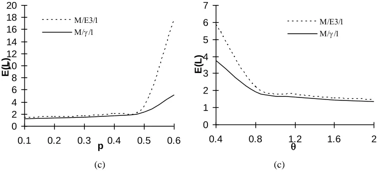
We have performed a numerical experiments by coding a computer program in software MATLAB to examine the effect of various parameters on E(L). The numerical results are displayed by figures 1-4 by taking exponential distributions for setup time, retrial time and vacation time. For bar diagrams depicted in figures 1 and 2, we fix the service time and repair time as an exponential distribution and obtained the results for E(L) by taking different sets of joining probabilities (h1,h2) for varying values of , p, and Graphs in figures 3 & 4 are drawn for different sets of Erlangian (k=3) and Gamma (k=0.8) distributions corresponding to both service time and repair time by varying same parameters.
We set the parameters for bar figures 1(a-c) & 2(a-c) as , p=0.2, sv=0.5, J=10. Figures 1(a), 1(b) & 1(c) depict the results for E(L) by varying& p, respectively. Initially we see that E(L) gradually increases but after some time it increases sharply for higher values of & p, respectively. It is clearly noticed that E(L) initially decreases sharply with and in figuresa), 2(b) & 2(c), respectively but later for higher values of parameters, it becomes almost constant. It is quite visible that as we increase joining probability, E(L) also increases in all figures 1(a-c) and 2(a-c), which is what we expect from real life experiences.
For the figures 3 and 4, we set the parameters as , p=0.2, sv=0.5, J=10. Similar pattern has been observed in figures 3(a-c) with respect to & p, respectively as we have obtained in figures 1(a-c). Figures 4(a-c) illustrate the same trend as we have seen in figures 2(a-c) by varying and respectively. In Figures 3 and 4, Erlangian distribution gives higher value for E(L) as comparison to Gamma distribution.
Overall we have concluded that
Expected number of jobs increases with joining probabilities (h1,h2), arrival rate (), feedback parameter (p) and failure rate ().
There is a decrement in expected number of jobs with service rate (), repair rate () and retrial rate (). Erlangian distribution gives higher value for expected number of jobs as comparison to Gamma distribution.
VIII. CONCLUSION
In the present study, a single unreliable server M/G/1 retrial queueing system with modified vacation and discouragement is considered. To obtain analytical expressions for various performance indices of interest, we employ generating function approach. The model with general retrial and modified vacation policy depicts more versatile congestion situations of communication networks, switching system, assembly lines, etc. apart from day-to-day life problems encountered at various service and distribution centers.
REFERENCES
[1] Abidini, M. A., Boxma, O. and Resting, J.“Analysis and optimization of vacation and polling models with retrials”, Per. Eva.,
Vol. 98, pp 52-69, 2016.
[2] Atencia, I. and Moreno, P.“Discrete time Geo[X]/GH/1 retrial queue with Bernoulli feedback”, Comput. Math.Appli., Vol.
47(8-9), pp. 1273-1294, 2004.
[3] Boxma, O.J. and Yechiali, U.“An M/G/1 queue with multiple types of feedback and gated vacations”, J. Appl.Prob. Vol. 34,
pp. 773-784, 1997.
[4] Falin G.“An M/G/1 retrial queue with an unreliable server and general repair times”, Perf. Eval., Vol. 67, Issue 7, pp.
569-582, 2010.
[5] Jain, M. and Sharma, P.“Finite capacity queueing system with queue dependent servers and discouragement”,Jnanabha, Vol.
38, pp. 1-12, 2008.
[6] Ke, J. C., Huang, K. B. and Pearn, W. L. “The randomized vacation policy for a batch arrival queue”, App.Math. Model., Vol.
34, Issue 6, pp. 1524-1538, 2010.
[7] Kulkarni, V.G. and Choi, B.D. “Retrial queues with server subject to breakdown and repair”, Queueing System,Vol. 7, pp.
191-208, 1990.
[8] Kumar, B. K., Vijayalakshmi, G., Krishanamoorthy, A. and Basha, S. S.“A single server feedback retrialqueue with
ISSN: 2231 – 5373
http://www.ijmttjournal.org
Page 19
[9] Kumar, K. B. and Madheswari, S.V. “MX/G/1 retrial queue with multiple vacations and starting failures”, OPSEARCH, Vol.
40(2), pp. 115-137, 2013.
[10]Rao, S.S. “Queueing with balking and reneging in M/G/1 systems, Metrika”, Vol. 12, pp. 173-188, 1968.
[11]Sharma, P. “Finite population loss and delay queue under no passing restriction and discouragement”, Elixir Appl. Math., Vol.
109, pp. 47940-47946, 2017.
[12]Sharma, P. “Unreliable server mx/g/1 queue with loss-delay, balking and second optional service”, Int. J.Engg,Iran, Vol. 30,
No. 2, pp. 243-252, 2017.
[13]Takacs, L. “A single server queue with feedback”, Bell. Syst. Tech. J., Vol. 42, pp. 505-519, 1963.
[14]Teghem, L. “Analysis of a single server queueing system with vacation periods”, Belgian J. Oper. Res., Vol.25, pp. 47-54,
1985.
[15]Upadhyaya, S. “Performance predication of a discrete-time batch arrival retrial queue with Bernoulli feedback”,App. Math.
Model., Vol. 283, pp. 108-119, 2016.
(a) (a)
(b) (b)
0 3 6 9 12 15 18 21 24
0.1 0.2 0.3 0.4 0.5 0.6
E
(L
)
h1=1,h2=1 h1=.9,h2=.9 h1=.8,h2=.8
0.0 0.5 1.0 1.5 2.0
2 4 6 8 10
E(L)
h1=1,h2=1
h1=.9,h2=.9 h1=.8,h2=.8
0 1 2 3 4 5 6
0 2 4 6 8 10 12
E
(L
)
h1=1,h2=1
h1=.9,h2=.9
h1=.8,h2=.8
0 1 2 3 4 5 6
3 6 9 12 15
E(L
)
h1=1,h2=1
h1=.9,h2=.9
ISSN: 2231 – 5373
http://www.ijmttjournal.org
Page 20
(c) (c)
Fig. 1: Effect of joining probability on E(L)Fig. 2: Effect of joining probability on E(L) by varying (a) (b) & (c) p by varying (a) (b) & (c)
(a) (a)
(b) (b)
0 1 2 3 4 5 6 7
0.1 0.2 0.3 0.4 0.5 0.6 0.7
E
(L
)
p h1=1,h2=1
h1=.9,h2=.9 h1=.8,h2=.8
0 1 2 3
0.2 0.4 0.6 0.8 1
E
(L
)
h1=1,h2=1
h1=.9,h2=.9 h1=.8,h2=.8
0 1 2 3 4 5 6 7
0.2 0.4 0.6 0.8 1
E
(L
)
M/E/ M/ /
0 1 2 3 4 5 6 7
4 6 8 10 12
E
(L
)
M/E/ M/ /
0 1 2 3 4 5 6 7 8
0 2 4 6 8 10
E
(L
)
M/E/ M/ /
0 5 10 15 20 25 30 35
0.3 0.6 0.9 1.2
E
(L
)
ISSN: 2231 – 5373
http://www.ijmttjournal.org
Page 21
(c) (c)
Fig. 3: Effect of different distribution on E(L) Fig. 4: Effect of different distribution on E(L) by varying (a) (b) & (c) p by varying (a) (b) & (c) 0
2 4 6 8 10 12 14 16 18 20
0.1 0.2 0.3 0.4 0.5 0.6
p
E
(L
)
M/E/ M/ /
0 1 2 3 4 5 6 7
0.4 0.8 1.2 1.6 2
E
(L
)