The Thirty-Third AAAI Conference on Artificial Intelligence (AAAI-19)
M2Det: A Single-Shot Object Detector
Based on Multi-Level Feature Pyramid Network
Qijie Zhao,
1Tao Sheng,
1Yongtao Wang,
1∗Zhi Tang,
1Ying Chen,
2Ling Cai,
2Haibin Ling
31Institute of Computer Science and Technology, Peking University, Beijing, P.R. China
2AI Labs, DAMO Academy, Alibaba Group
3Computer and Information Sciences Department, Temple University
{zhaoqijie, shengtao, wyt, tangzhi}@pku.edu.cn,
{cailing.cl, chenying.ailab}@alibaba-inc.com,{hbling}@temple.edu
Abstract
Feature pyramids are widely exploited by both the state-of-the-art one-stage object detectors (e.g., DSSD, RetinaNet, RefineDet) and the two-stage object detectors (e.g., Mask R-CNN, DetNet) to alleviate the problem arising from scale variation across object instances. Although these object de-tectors with feature pyramids achieve encouraging results, they have some limitations due to that they only simply con-struct the feature pyramid according to the inherent multi-scale, pyramidal architecture of the backbones which are originally designed for object classification task. Newly, in this work, we present Multi-Level Feature Pyramid Network (MLFPN) to construct more effective feature pyramids for detecting objects of different scales. First, we fuse multi-level features (i.e. multiple layers) extracted by backbone as the base feature. Second, we feed the base feature into a block of alternating joint Thinned U-shape Modules and Feature Fusion Modules and exploit the decoder layers of each U-shape module as the features for detecting objects. Finally, we gather up the decoder layers with equivalent scales (sizes) to construct a feature pyramid for object detection, in which every feature map consists of the layers (features) from mul-tiple levels. To evaluate the effectiveness of the proposed MLFPN, we design and train a powerful end-to-end one-stage object detector we call M2Det by integrating it into the ar-chitecture of SSD, and achieve better detection performance than state-of-the-art one-stage detectors. Specifically, on MS-COCO benchmark, M2Det achieves AP of 41.0 at speed of 11.8 FPS with single-scale inference strategy and AP of 44.2 with multi-scale inference strategy, which are the new state-of-the-art results among one-stage detectors. The code will be made available on https://github.com/qijiezhao/M2Det.
Introduction
Scale variation across object instances is one of the major challenges for the object detection task (Lin et al. 2017a; He et al. 2015; Singh and Davis 2018), and usually there are two strategies to solve the problem arising from this chal-lenge. The first one is to detect objects in an image pyramid
(i.e.a series of resized copies of the input image) (Singh and
Davis 2018), which can only be exploited at the testing time.
∗
Corresponding author.
Copyright c2019, Association for the Advancement of Artificial Intelligence (www.aaai.org). All rights reserved.
(a) SSD-style feature pyramid
detect detect detect detect
(b) FPN-style feature pyramid
(d) Our multi-level feature pyramid
detect detect
detect
(c) STDN-style feature pyramid
Scale
transfer …
detect detect detect detect detect
detect detect detect detect detect detect
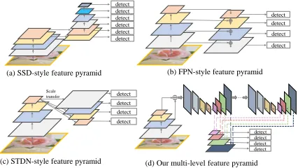
Figure 1: Illustrations of four kinds of feature pyramids.
Obviously, this solution will greatly increase memory and computational complexity, thus the efficiency of such object detectors drop dramatically. The second one is to detect ob-jects in a feature pyramid extracted from the input image (Liu et al. 2016; Lin et al. 2017a), which can be exploited at both training and testing phases. Compared with the first solution that uses an image pyramid, it has less memory and computational cost. Moreover, the feature pyramid con-structing module can be easily integrated into the state-of-the-art deep neural networks based detectors, yielding an end-to-end solution.
Although the object detectors with feature pyramids (Liu et al. 2016; Lin et al. 2017a; 2017b; He et al. 2017) achieve encouraging results, they still have some limitations due to that they simply construct the feature pyramid according to the inherent multi-scale, pyramidal architecture of the backbones which are actually designed for object classifi-cation task. For example, as illustrated in Fig. 1, SSD (Liu et al. 2016) directly and independently uses two layers of
the backbone (i.e.VGG16) and four extra layers obtained
representa-tive enough for the object detection task, since they are sim-ply constructed from the layers (features) of the backbone designed for object classification task. Second, each feature map in the pyramid (used for detecting objects in a spe-cific range of size) is mainly or even solely constructed from single-level layers of the backbone, that is, it mainly or only contains single-level information. In general, high-level fea-tures in the deeper layers are more discriminative for clas-sification subtask while low-level features in the shallower layers can be helpful for object location regression sub-task. Moreover, low-level features are more suitable to character-ize objects with simple appearances while high-level fea-tures are appropriate for objects with complex appearances. In practice, the appearances of the object instances with sim-ilar size can be quite different. For example, a traffic light and a faraway person may have comparable size, and the ap-pearance of the person is much more complex. Hence, each feature map (used for detecting objects in a specific range of size) in the pyramid mainly or only consists of single-level features will result in suboptimal detection performance.
The goal of this paper is to construct a more effective fea-ture pyramid for detecting objects of different scales, while avoid the limitations of the existing methods as above men-tioned. As shown in Fig. 2, to achieve this goal, we first fuse
multi-level features (i.e.multiple layers) extracted by
back-bone as base feature, and then feed it into a block of alter-nating joint Thinned U-shape Modules(TUM) and Feature Fusion Modules(FFM) to extract more representative, multi-level multi-scale features. It is worth noting that, decoder layers in each U-shape Module share a similar depth. Fi-nally, we gather up the feature maps with equivalent scales to construct the final feature pyramid for object detection. Ob-viously, decoder layers that form the final feature pyramid are much deeper than the layers in the backbone, namely, they are more representative. Moreover, each feature map in the final feature pyramid consists of the decoder layers from multiple levels. Hence, we call our feature pyramid block Multi-Level Feature Pyramid Network (MLFPN).
To evaluate the effectiveness of the proposed MLFPN, we design and train a powerful end-to-end one-stage object de-tector we call M2Det (according to that it is built upon multi-level and multi-scale features) by integrating MLFPN into the architecture of SSD (Liu et al. 2016). M2Det achieves
the new state-of-the-art result (i.e.AP of 41.0 at speed of
11.8 FPS with single-scale inference strategy and AP of 44.2 with multi-scale inference strategy), outperforming the one-stage detectors on MS-COCO (Lin et al. 2014) benchmark.
Related Work
Researchers have put plenty of efforts into improving the detection accuracy of objects with various scales – no mat-ter what kind of detector it is, either an one-stage detector or a two-stage one. To the best of our knowledge, there are mainly two strategies to tackle this scale-variation problem.
The first one is featurizing image pyramids (i.e.a
ries of resized copies of the input image) to produce se-mantically representative multi-scale features. Features from images of different scales yield predictions separately and these predictions work together to give the final prediction.
In terms of recognition accuracy and localization precision, features from various-sized images do surpass features that are based merely on single-scale images. Methods such as (Shrivastava et al. 2016) and SNIP (Singh and Davis 2018) employed this tactic. Despite the performance gain, such a strategy could be costly time-wise and memory-wise, which forbid its application in real-time tasks. Considering this major drawback, methods such as SNIP (Singh and Davis 2018) can choose to only employ featurized image pyramids during the test phase as a fallback, whereas other methods including Fast R-CNN (Girshick 2015) and Faster R-CNN (Ren et al. 2015) chose not to use this strategy by default.
The second one is detecting objects in thefeature
pyra-midextracted from inherent layers within the network while
merely taking a single-scale image. This strategy demands significantly less additional memory and computational cost than the first one, enabling deployment during both the train-ing and test phases in real-time networks. Moreover, the fea-ture pyramid constructing module can be easily revised and fit into state-of-the-art deep neural networks based detectors. MS-CNN (Cai et al. 2016), SSD (Liu et al. 2016), DSSD (Fu et al. 2017), FPN (Lin et al. 2017a), YOLOv3 (Redmon and Farhadi 2018), RetinaNet (Lin et al. 2017b), and RefineDet (Zhang et al. 2018) adopted this tactic in different ways.
To the best of our knowledge, MS-CNN (Cai et al. 2016) proposed two sub-networks and first incorporated multi-scale features into deep convolutional neural networks for object detection. The proposal sub-net exploited feature maps of several resolutions to detect multi-scale objects in an image. SSD (Liu et al. 2016) exploited feature maps from the later layers of VGG16 base-net and extra feature lay-ers for predictions at multiple scales. FPN (Lin et al. 2017a) utilized lateral connections and a top-down pathway to pro-duce a feature pyramid and achieved more powerful repre-sentations. DSSD (Fu et al. 2017) implemented deconvolu-tion layers for aggregating context and enhancing the high-level semantics for shallow features. RefineDet (Zhang et al. 2018) adopted two-step cascade regression, which achieves a remarkable progress on accuracy while keeping the effi-ciency of SSD.
Proposed Method
The overall architecture of M2Det is shown in Fig. 2. M2Det uses the backbone and the Multi-Level Feature Pyramid Net-work (MLFPN) to extract features from the input image, and then similar to SSD, produces dense bounding boxes and category scores based on the learned features, followed by the non-maximum suppression (NMS) operation to pro-duce the final results. MLFPN consists of three modules,
i.e.Feature Fusion Module (FFM), Thinned U-shape
FFM1 Pr ed iction l ay er s
Backbone network Base feature
Multi-Level Feature Pyramid SF AM FFMv2 FFMv2 O u tp u t: th e max o n e Ou tp u t: th e ma x o n e . . . . TUM . . . . MLFPN TUM TUM shallow medium deep 320×320 40×40 5×5 10×10 20×20 40×40
Figure 2: An overview of the proposed M2Det(320×320). M2Det utilizes the backbone and the Multi-level Feature Pyramid
Network (MLFPN) to extract features from the input image, and then produces dense bounding boxes and category scores. In MLFPN, FFMv1 fuses feature maps of the backbone to generate the base feature. Each TUM generates a group of multi-scale features, and then the alternating joint TUMs and FFMv2s extract multi-level multi-scale features. Finally, SFAM aggregates the features into a multi-level feature pyramid. In practice, we use 6 scales and 8 levels.
Feature pyramid 1 Feature pyramid 2 Feature pyramid t …. Same-scale concatenate …. ….
40×40×1024 20x20x1024 10×10×1024
Shallow level
Medium level
Deep level
1×1×1024 1×1×1024
Reweighting
20×20×1024
Shallow medium deep
Figure 3: Illustration of Scale-wise Feature Aggregation Module. The first stage of SFAM is to concatenate features with equivalent scales along channel dimension. Then the second stage uses SE attention to aggregate features in an adaptive way.
Conv 512,3x3,1x1,256 Conv 1024,1x1,1x1,512 Upsample 2x2 Concat (512,40,40) (1024,20,20) (768,40,40) Conv 768,1x1,1x1,128 Concat (768,40,40) (128,40,40) (256,40,40) (a) (b) Conv 256,3x3,2x2,256 Conv 256,3x3,2x2,256 Conv 256,3x3,2x2,256 Conv 256,3x3,2x2,256 Conv 256,3x3,1x1,256 Conv 256,3x3,1x1,256 Conv 256,3x3,1x1,256 Conv 256,3x3,1x1,256 Conv 256,3x3,2x2,256 Conv 256,3x3,1x1,256 Conv 256,1x1,1x1,128 Conv 256,1x1,1x1,128 Conv 256,1x1,1x1,128 Conv 256,1x1,1x1,128 Conv 256,1x1,1x1,128 (256,40,40) (c) Conv 256,1x1,1x1,128
(128,40,40) (128,20,20) (128,10,10) (128,5,5) (128,3,3) (128,1,1)
Conv
256,3x3,1x1,128
Conv+BN+ReLU layers
Input_channel:256;output_channel:128; Kernel_size:3x3;Stride_size:1x1
Blinear Upsample + ele-wise sum
Brief indication:
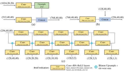
Figure 4: Structural details of some modules. (a) FFMv1, (b) FFMv2, (c) TUM. The inside numbers of each block de-note: input channels, Conv kernel size, stride size, output channels.
network configurations in M2Det are introduced in the fol-lowing.
Multi-level Feature Pyramid Network
As shown in Fig. 2, MLFPN contains three parts. Firstly, FFMv1 fuses shallow and deep features to produce the base
feature,e.g., conv4 3 and conv5 3 of VGG (Simonyan and
Zisserman 2015), which provide multi-level semantic infor-mation for MLFPN. Secondly, several TUMs and FFMv2 are stacked alternately. Specifically, each TUM generates
several feature maps with different scales. The FFMv2 fuses the base feature and the largest output feature map of the previous TUM. And the fused feature maps are fed to the next TUM. Note that the first TUM has no prior knowledge
of any other TUMs, so it only learns fromXbase. The output
multi-level multi-scale features are calculated as:
[xl1,xl2, ...,xli] =
Tl(Xbase), l= 1
Tl(F(Xbase,xil−1)), l= 2...L
, (1)
whereXbase denotes the base feature,xli denotes the
fea-ture with thei-th scale in thel-th TUM,Ldenotes the
num-ber of TUMs, Tldenotes thel-th TUM processing, andF
denotes FFMv1 processing. Thirdly, SFAM aggregates the multi-level multi-scale features by a scale-wise feature con-catenation operation and a channel-wise attention mecha-nism.
FFMsFFMs fuse features from different levels in M2Det,
fused feature for the next TUM. Structural details of FFMv1 and FFMv2 are shown in Fig. 4 (a) and (b), respectively.
TUMsDifferent from FPN (Lin et al. 2017a) and
Reti-naNet (Lin et al. 2017b), TUM adopts a thinner U-shape structure as illustrated in Fig. 4 (c). The encoder is a se-ries of 3x3 convolution layers with stride 2. And the de-coder takes the outputs of these layers as its reference set of feature maps, while the original FPN chooses the output of the last layer of each stage in ResNet backbone. In addition, we add 1x1 convolution layers after upsample and element-wise sum operation at the decoder branch to enhance learn-ing ability and keep smoothness for the features (Lin, Chen, and Yan 2014). All of the outputs in the decoder of each TUM form the multi-scale features of the current level. As a whole, the outputs of stacked TUMs form the multi-level multi-scale features, while the front TUM mainly provides shallow-level features, the middle TUM provides medium-level features, and the back TUM provides deep-medium-level fea-tures.
SFAM SFAM aims to aggregate the level
multi-scale features generated by TUMs into a multi-level fea-ture pyramid as shown in Fig. 3. The first stage of SFAM is to concatenate features of the equivalent scale together along the channel dimension. The aggregated feature
pyra-mid can be presented as X = [X1,X2, ...,Xi], where
Xi = Concat(x1i,x
2
i, ...,x L
i) ∈ R
Wi×Hi×C refers to the
features of thei-th largest scale. Here, each scale in the
ag-gregated pyramid contains features from multi-level depths. However, simple concatenation operations are not adaptive enough. In the second stage, we introduce a channel-wise attention module to encourage features to focus on chan-nels that they benefit most. Following SE block (Hu, Shen, and Sun 2017), we use global average pooling to generate
channel-wise statisticsz ∈RC at the squeeze step. And to
fully capture channel-wise dependencies, the following ex-citation step learns the attention mechanism via two fully connected layers:
s=Fex(z,W) =σ(W2δ(W1z)), (2)
whereσrefers to the ReLU function,δrefers to the sigmoid
function,W1 ∈ R
C
r×C,W2 ∈RC× C
r, r is the reduction
ratio (r = 16in our experiments). The final output is
ob-tained by reweighting the inputXwith activations:
˜
Xci =Fscale(Xic, sc) =sc·Xci, (3)
whereX˜i = [ ˜X1i,X˜2i, ...,X˜Ci ], each of the features is
en-hanced or weakened by the rescaling operation.
Network Configurations
We assemble M2Det with two kinds of backbones (Si-monyan and Zisserman 2015; He et al. 2016). Before train-ing the whole network, the backbones need to be pre-trained on the ImageNet 2012 dataset (Russakovsky et al. 2015). All of the default configurations of MLFPN contain 8 TUMs, each TUM has 5 striding-Convs and 5 Upsample operations, so it will output features with 6 scales. To reduce the number of parameters, we only allocate 256 channels to each scale of their TUM features, so that the network could be easy
to train on GPUs. As for input size, we follow the original
SSD, RefineDet and RetinaNet,i.e.,320, 512 and 800.
At the detection stage, we add two convolution layers to each of the 6 pyramidal features to achieve location re-gression and classification respectively. The detection scale ranges of the default boxes of the six feature maps follow the setting of the original SSD. And when input size is
800×800, the scale ranges increase proportionally except
keeping the minimum size of the largest feature map. At each pixel of the pyramidal features, we set six anchors with three ratios entirely. Afterward, we use a probability score of 0.05 as threshold to filter out most anchors with low scores. Then we use soft-NMS (Bodla et al. 2017) with a linear ker-nel for post-processing, leaving more accurate boxes. De-creasing the threshold to 0.01 can generate better detection results, but it will slow down the inference time a lot, we do not consider it for pursuing better practical values.
Experiments
In this section, we present experimental results on the bounding box detection task of the challenging MS-COCO benchmark. Following the protocol in MS-COCO, we use
thetrainval35kset for training, which is a union of 80k
images fromtrainsplit and a random 35 subset of images
from the 40k image valsplit. To compare with
state-of-the-art methods, we report COCO AP on the test-dev
split, which has no public labels and requires the use of the evaluation server. And then, we report the results of ablation
studies evaluated on theminivalsplit for convenience.
Our experiment section includes 4 parts: (1) introducing implement details about the experiments; (2) demonstrating the comparisons with state-of-the-art approaches; (3) abla-tion studies about M2Det; (4) comparing different settings about the internal structure of MLFPN and introducing sev-eral version of M2Det.
Implementation details
For all experiments based on M2Det, we start training with warm-up strategy for 5 epochs, initialize the learning rate as
2×10⁻³, and then decrease it to2×10−4and2×10−5at
90 epochs and 120 epochs, and stop at 150 epochs. M2Det is
developed with PyTorch v0.4.01. When input size is 320 and
512, we conduct experiments on a machine with 4 NVIDIA Titan X GPUs, CUDA 9.2 and cuDNN 7.1.4, while for input size of 800, we train the network on NVIDIA Tesla V100 to get results faster. The batch size is set to 32 (16 each for 2 GPUs, or 8 each for 4 GPUs). On NVIDIA Titan Xp that has 12 GB memory, the training performance is limited if batch size on a single GPU is less than 5. Notably, for Resnet101, M2Det with the input size of 512 is not only limited in the batch size (only 4 is available), but also takes a long time to train, so we train it on V100.
For training M2Det with the VGG-16 backbone when
in-put size is 320×320 and 512×512 on 4 Titan X devices,
the total training time costs 3 and 6 days respectively, and
with the ResNet-101 backbone when 320×320 costs 5 days.
While for training M2Det with ResNet-101 when input
1
Method Backbone Input size MultiScale FPS Avg. Precision, IoU: Avg. Precision, Area: 0.5:0.95 0.5 0.75 S M L
two-stage:
Faster R-CNN (Ren et al. 2015) VGG-16 ∼1000×600 False 7.0 21.9 42.7 - - - -OHEM++ (Shrivastava et al. 2016) VGG-16 ∼1000×600 False 7.0 25.5 45.9 26.1 7.4 27.7 40.3 R-FCN (Dai et al. 2016) ResNet-101 ∼1000×600 False 9 29.9 51.9 - 10.8 32.8 45.0 CoupleNet (Zhu et al. 2017) ResNet-101 ∼1000×600 False 8.2 34.4 54.8 37.2 13.4 38.1 50.8 Faster R-CNN w FPN (Lin et al. 2017a) Res101-FPN ∼1000×600 False 6 36.2 59.1 39.0 18.2 39.0 48.2 Deformable R-FCN (Dai et al. 2017) Inc-Res-v2 ∼1000×600 False - 37.5 58.0 40.8 19.4 40.1 52.5 Mask R-CNN (He et al. 2017) ResNeXt-101 ∼1280×800 False 3.3 39.8 62.3 43.4 22.1 43.2 51.2 Fitness-NMS (Tychsen-Smith and Petersson 2018) ResNet-101 ∼1024×1024 True 5.0 41.8 60.9 44.9 21.5 45.0 57.5 Cascade R-CNN (Cai and Vasconcelos 2018) Res101-FPN ∼1280×800 False 7.1 42.8 62.1 46.3 23.7 45.5 55.2
SNIP (Singh and Davis 2018) DPN-98 - True - 45.7 67.3 51.1 29.3 48.8 57.1
one-stage:
SSD300* (Liu et al. 2016) VGG-16 300×300 False 43 25.1 43.1 25.8 6.6 25.9 41.4
RON384++ (Kong et al. 2017) VGG-16 384×384 False 15 27.4 49.5 27.1 - -
-DSSD321 (Fu et al. 2017) ResNet-101 321×321 False 9.5 28.0 46.1 29.2 7.4 28.1 47.6 RetinaNet400 (Lin et al. 2017b) ResNet-101 ∼640×400 False 12.3 31.9 49.5 34.1 11.6 35.8 48.5 RefineDet320 (Zhang et al. 2018) VGG-16 320×320 False 38.7 29.4 49.2 31.3 10.0 32.0 44.4 RefineDet320 (Zhang et al. 2018) ResNet-101 320×320 True - 38.6 59.9 41.7 21.1 41.7 52.3 M2Det (Ours) VGG-16 320×320 False 33.4 33.5 52.4 35.6 14.4 37.6 47.6 M2Det (Ours) VGG-16 320×320 True - 38.9 59.1 42.4 24.4 41.5 47.6 M2Det (Ours) ResNet-101 320×320 False 21.7 34.3 53.5 36.5 14.8 38.8 47.9 M2Det (Ours) ResNet-101 320×320 True - 39.7 60.0 43.3 25.3 42.5 48.3 YOLOv3 (Redmon and Farhadi 2018) DarkNet-53 608×608 False 19.8 33.0 57.9 34.4 18.3 35.4 41.9 SSD512* (Liu et al. 2016) VGG-16 512×512 False 22 28.8 48.5 30.3 10.9 31.8 43.5 DSSD513 (Fu et al. 2017) ResNet-101 513×513 False 5.5 33.2 53.3 35.2 13.0 35.4 51.1 RetinaNet500 (Lin et al. 2017b) ResNet-101 ∼832×500 False 11.1 34.4 53.1 36.8 14.7 38.5 49.1 RefineDet512 (Zhang et al. 2018) VGG-16 512×512 False 22.3 33.0 54.5 35.5 16.3 36.3 44.3 RefineDet512 (Zhang et al. 2018) ResNet-101 512×512 True - 41.8 62.9 45.7 25.6 45.1 54.1 CornerNet (Law and Deng 2018) Hourglass 512×512 False 4.4 40.5 57.8 45.3 20.8 44.8 56.7 CornerNet (Law and Deng 2018) Hourglass 512×512 True - 42.1 57.8 45.3 20.8 44.8 56.7 M2Det (Ours) VGG-16 512×512 False 18.0 37.6 56.6 40.5 18.4 43.4 51.2 M2Det (Ours) VGG-16 512×512 True - 42.9 62.5 47.2 28.0 47.4 52.8 M2Det (Ours) ResNet-101 512×512 False 15.8 38.8 59.4 41.7 20.5 43.9 53.4 M2Det (Ours) ResNet-101 512×512 True - 43.9 64.4 48.0 29.6 49.6 54.3 RetinaNet800 (Lin et al. 2017b) Res101-FPN ∼1280×800 False 5.0 39.1 59.1 42.3 21.8 42.7 50.2 M2Det (Ours) VGG-16 800×800 False 11.8 41.0 59.7 45.0 22.1 46.5 53.8 M2Det (Ours) VGG-16 800×800 True - 44.2 64.6 49.3 29.2 47.9 55.1
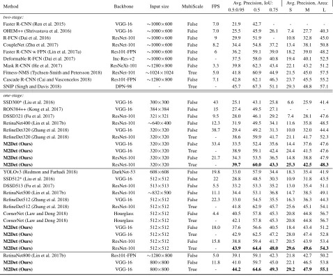
Table 1: Detection accuracy comparisons in terms of mAP percentage onMS COCOtest-dev set.
size is 512×512 on 2 V100 devices, it costs 11 days. The
most accurate model is M2Det with the VGG backbone and
800×800 input size, it costs 14 days.
Comparison with State-of-the-art
We compare the experimental results of the proposed M2Det with state-of-the-art detectors in Table 1. For these experi-ments, we use 8 TUMs and set 256 channels for each TUM. The main information involved in the comparison includes the input size of the model, the test method (whether it uses multi-scale strategy), the speed of the model, and the test results. Test results of M2Det with 10 different setting ver-sions are reported in Table 1, which are produced by testing
it on MS-COCO test-devsplit, with a single NVIDIA
Titan X PASCAL and the batch size 1. Other statistical re-sults stem from references. It is noteworthy that, M2Det-320 with VGG backbone achieves AP of 38.9, which has sur-passed most object detectors with more powerful backbones
and larger input size,e.g., AP of Deformable R-FCN (Dai et
al. 2017) is 37.5, AP of Faster R-CNN with FPN is 36.2.
As-sembled with ResNet-101 can further improve M2Det, the single-scale version obtains AP of 38.8, which is competi-tive with state-of-the-art two-stage detectors Mask R-CNN (He et al. 2017). In addition, based on the optimization of PyTorch, it can run at 15.8 FPS. RefineDet (Zhang et al. 2018) inherits the merits of one-stage detectors and two-stage detectors, gets AP of 41.8, CornerNet (Law and Deng 2018) proposes key point regression for detection and bor-rows the advantages of Hourglass (Newell, Yang, and Deng 2016) and focal loss (Lin et al. 2017b), thus gets AP of 42.1. In contrast, our proposed M2Det is based on the regression method of original SSD, with the assistance of Multi-scale Multi-level features, obtains 44.2 AP, which exceeds all one-stage detectors. Most approaches do not compare the speed of multi-scale inference strategy due to different methods or tools used, so we also only focus on the speed of single-scale inference methods.
state-of-the-art one-stage detectors and two-stage detectors. Cor-nerNet with Hourglass has 201M parameters, Mask R-CNN (He et al. 2017) with ResNeXt-101-32x8d-FPN (Xie et al. 2017) has 205M parameters. By contrast, M2Det800-VGG has only 147M parameters. Besides, consider the compari-son of depth, it is also not dominant.
Ablation study
Since M2Det is composed of multiple subcomponents, we need to verify each of its effectiveness to the final perfor-mance. The baseline is a simple detector based on the
orig-inal SSD, with 320×320 input size and VGG-16 reduced
backbone.
+ 1 s-TUM X
+ 8 s-TUM X
+ 8 TUM X X X X
+ Base feature X X X
+ SFAM X X
VGG16⇒Res101 X
AP 25.8 27.5 30.6 30.8 32.7 33.2 34.1 AP50 44.7 45.2 50.0 50.3 51.9 52.2 53.7
APsmall 7.2 7.7 13.8 13.7 13.9 15.0 15.9
APmedium 27.4 28.0 35.3 35.3 37.9 38.2 39.5
APlarge 41.4 47.0 44.5 44.8 48.8 49.1 49.3
Table 2: Ablation study of M2Det. The detection results are
evaluated onminivalset
TUMTo demonstrate the effectiveness of TUM, we
con-duct three experiments. First, following DSSD, we extend the baseline detector with a series of Deconv layers, and the AP has improved from 25.8 to 27.5 as illustrated in the third column in Table 2. Then we replace with MLFPN into it. As for the U-shape module, we firstly stack 8 s-TUMs, which
is modified to decrease the 1×1 Convolution layers shown
in Fig. 4, then the performance has improved 3.1 compared with the last operation, shown in the forth column in Table 2. Finally, replacing TUM by s-TUM in the fifth column has reached the best performance, it comes to AP of 30.8.
Base featureAlthough stacking TUMs can improve
de-tection, but it is limited by input channels of the first TUM. That is, decreasing the channels will drop the abstraction of MLFPN, while increasing them will highly increase the pa-rameters number. Instead of using base feature only once, We afferent base feature at the input of each TUM to allevi-ate the problem. For each TUM, the embedded base feature provides necessary localization information since it contains shallow features. The AP percentage increases to 32.7, as shown in the sixth column in Table 2.
SFAMAs shown in the seventh column in Table 2,
com-pared with the architecture that without SFAM, all evalua-tion metrics have been upgraded. Specifically, all boxes in-cluding small, medium and large become more accurate.
Backbone featureAs in many visual tasks, we observe
a noticeable AP gain from33.2to34.1when we use
well-tested ResNet-101 (He et al. 2016) instead of VGG-16 as the backbone network. As shown in Table 2, such observation remains true and consistent with other AP metrics.
TUMs Channels Params(M) AP AP50 AP75
2 256 40.1 30.5 50.5 32.0
2 512 106.5 32.1 51.8 34.0
4 128 34.2 29.8 49.7 31.2
4 256 60.2 31.8 51.4 33.0
4 512 192.2 33.4 52.6 34.2
8 128 47.5 31.8 50.6 33.6
8 256 98.9 33.2 52.2 35.2
8 512 368.8 34.0 52.9 36.4
16 128 73.9 32.5 51.7 34.4
16 256 176.8 33.6 52.6 35.7
Table 3: Different configurations of MLFPN in M2Det. The
backbone is VGG and input image is 320×320.
Variants of MLFPN
The Multi-scale Multi-level Features have been proved to be effective. But what is the boundary of the improvement brought by MLFPN? Step forward, how to design TUM and how many TUMs should be OK? We implement a group of variants to find the regular patterns. To be more specific, we fix the backbone as VGG-16 and the input image size as 320x320, and then tune the number of TUMs and the num-ber of internal channels of each TUM.
As shown in Table 3, M2Det with different configurations
of TUMs is evaluated on COCO minival set.
Compar-ing the number of TUMs when fixCompar-ing the channels,e.g.,256,
it can be concluded that stacking more TUMs brings more promotion in terms of detection accuracy. Then fixing the number of TUMs, no matter how many TUMs are assem-bled, more channels consistently benefit the results. Further-more, assuming that we take a version with 2 TUMS and 128 channels as the baseline, using more TUMs could bring larger improvement compared with increasing the internal channels, while the increase in parameters remains similar.
Speed
We compare the inference speed of M2Det with state-of-the-art approaches. Since VGG-16 (Simonyan and Zisser-man 2015) reduced backbone has removed FC layers, it is very fast to use it for extracting base feature. We set the batch size to 1, take the sum of the CNN time and NMS time of 1000 images, and divide by 1000 to get the inference time of a single image. Specifically, we assemble VGG16-reduced to M2Det and propose the fast version M2Det with
the input size 320×320, the standard version M2Det with
512×512 input size and the most accurate version M2Det
with 800×800 input size. Based on the optimization of
B*
Method mAP time
[A] YOLOv3 – 608 33.0 51 [B] SSD – 321 28.0 61 [B*] SSD – 321 28.2 22 [C] DSSD – 321 28.0 85 [D] R-FCN 29.9 85 [E] SSD – 513 31.2 125 [E*] SSD – 513 31.0 37 [F] DSSD – 513 33.2 156 [G] FPN FRCN 36.2 172 [H*] CornerNet 40.5 228 RetinaNet 39.1 198 [*]RefineDet 36.7 110
M2Det 41.0 84.7
(*) Tested on our machine for fair comparison 28
30 32 34 36 38 40
C
OC
O
AP
Inference time (ms)
100 150 200
50 A
B C
D E
F G M2Det512-vgg
mAP: 37.6 Time: 55.5ms M2Det320-vgg mAP: 33.5 Time: 29.9ms
M2Det800-vgg mAP: 41.0 Time: 84.7ms
E*
H*
Figure 5: Speed (ms) vs. accuracy (mAP) on COCOtest-dev.
level
scale
Shallow->Deep
Traffic sign Car Pedestrian
Figure 6: Example activation values of scale multi-level features. Best view in color.
Discussion
We think the detection accuracy improvement of M2Det is mainly brought by the proposed MLFPN. On one hand, we fuse multi-level features extracted by backbone as the base feature, and then feed it into a block of alternating joint Thinned U-shape Modules and Feature Fusion Mod-ules to extract more representative, multi-level multi-scale
features, i.e. the decoder layers of each TUM. Obviously,
these decoder layers are much deeper than the layers in the backbone, and thus more representative for object detection. Contrasted with our method, the existing detectors (Zhang et al. 2018; Lin et al. 2017a; Fu et al. 2017) just use the lay-ers of the backbone or extra laylay-ers with few depth increase. Hence, our method can achieve superior detection perfor-mance. On the other hand, each feature map of the multi-level feature pyramid generated by the SFAM consists of the decoder layers from multiple levels. In particular, at each scale, we use multi-level features to detect objects, which
would be better forhandling appearance-complexity
vari-ation across object instances.
To verify that the proposed MLFPN can learn effective feature for detecting objects with different scales and large appearance variation, we visualize the activation values of the summation output of SFAM module along scale and level dimensions, such an example shown in Fig. 6. The in-put image contains two persons, two cars and a traffic light.
Moreover, the sizes of the two persons are different, as well as the two cars. And the traffic light, the smaller person and the smaller car have similar sizes. We can find that: 1) com-pared with the smaller person, the larger person has strongest activation value at the feature map of large scale, so as to the smaller car and larger car; 2) the traffic light, the smaller per-son and the smaller car have strongest activation value at the feature maps of the same scale; 3) the persons, the cars and the traffic light have strongest activation value at the highest-level, middle-highest-level, lowest-level feature maps respectively. This example presents that: 1) our method learns very ef-fective features to handle scale variation and appearance-complexity variation across object instances; 2) it is neces-sary to use multi-level features to detect objects with similar size.
Conclusion
In this work, a novel method called Multi-Level Feature Pyramid Network (MLFPN) is proposed to construct ef-fective feature pyramids for detecting objects of different scales. MLFPN consists of several novel modules. First,
multi-level features (i.e.multiple layers) extracted by
back-bone are fused by a Feature Fusion Module (FFMv1) as the base feature. Second, the base feature is fed into a block of alternating joint Thinned U-shape Modules (TUMs) and Feature Fusion Modules (FFMv2s) and level
multi-scale features (i.e. the decoder layers of each TUM) are
extracted. Finally, the extracted multi-level multi-scale fea-tures with the same scale (size) are aggregated to construct a feature pyramid for object detection by a Scale-wise Feature Aggregation Module (SFAM). A powerful end-to-end one-stage object detector called M2Det is designed based on the proposed MLFPN, which achieves a new state-of-the-art
re-sult (i.e.AP of 41.0 at speed of 11.8 FPS with single-scale
inference strategy and AP of 44.2 with multi-scale infer-ence strategy) among the one-stage detectors on MS-COCO benchmark. Additional ablation studies further demonstrate the effectiveness of the proposed architecture and the novel modules.
Acknowledgements
This work is supported by National Natural Science Foun-dation of China under Grant 61673029. This work is also a research achievement of Key Laboratory of Science, Tech-nology and Standard in Press Industry (Key Laboratory of Intelligent Press Media Technology).
References
Bodla, N.; Singh, B.; Chellappa, R.; and Davis, L. S. 2017. Soft-nms - improving object detection with one line of code. InICCV 2017, 5562–5570.
Cai, Z., and Vasconcelos, N. 2018. Cascade r-cnn: Delving
into high quality object detection. InCVPR 2018.
Cai, Z.; Fan, Q.; Feris, R. S.; and Vasconcelos, N. 2016. A unified multi-scale deep convolutional neural network for
Dai, J.; Li, Y.; He, K.; and Sun, J. 2016. R-FCN: Object detection via region-based fully convolutional networks. In
NIPS 2016, 379–387.
Dai, J.; Qi, H.; Xiong, Y.; Li, Y.; Zhang, G.; Hu, H.; and
Wei, Y. 2017. Deformable convolutional networks. InICCV
2017, 764–773.
Fu, C.; Liu, W.; Ranga, A.; Tyagi, A.; and Berg, A. C.
2017. DSSD : Deconvolutional single shot detector. CoRR
abs/1701.06659.
Girshick, R. B. 2015. Fast R-CNN. InICCV 2015, 1440–
1448.
He, K.; Zhang, X.; Ren, S.; and Sun, J. 2015. Spatial
pyramid pooling in deep convolutional networks for visual
recognition.IEEE TPAMI.37(9):1904–1916.
He, K.; Zhang, X.; Ren, S.; and Sun, J. 2016. Deep residual
learning for image recognition. InCVPR 2016, 770–778.
He, K.; Gkioxari, G.; Doll´ar, P.; and Girshick, R. 2017.
Mask R-CNN. InICCV 2017, 2980–2988. IEEE.
Hu, J.; Shen, L.; and Sun, G. 2017. Squeeze-and-excitation
networks. CoRRabs/1709.01507.
Huang, G.; Liu, Z.; Van Der Maaten, L.; and Weinberger, K. Q. 2017. Densely connected convolutional networks. In
CVPR 2017, volume 1, 3.
Kong, T.; Sun, F.; Yao, A.; Liu, H.; Lu, M.; and Chen, Y. 2017. RON: reverse connection with objectness prior
net-works for object detection. InCVPR 2017, 5244–5252.
Law, H., and Deng, J. 2018. Cornernet: Detecting objects as
paired keypoints. InECCV 2018.
Lin, T.; Maire, M.; Belongie, S. J.; Hays, J.; Perona, P.; Ra-manan, D.; Doll´ar, P.; and Zitnick, C. L. 2014. Microsoft
COCO: common objects in context. InECCV 2014, 740–
755.
Lin, T.; Doll´ar, P.; Girshick, R. B.; He, K.; Hariharan, B.; and Belongie, S. J. 2017a. Feature pyramid networks for
object detection. InCVPR 2017, 936–944.
Lin, T.; Goyal, P.; Girshick, R. B.; He, K.; and Doll´ar, P.
2017b. Focal loss for dense object detection. InICCV 2017,
2999–3007.
Lin, M.; Chen, Q.; and Yan, S. 2014. Network in network. InICLR 2014.
Liu, W.; Anguelov, D.; Erhan, D.; Szegedy, C.; Reed, S. E.; Fu, C.; and Berg, A. C. 2016. SSD: single shot multibox
detector. InECCV 2016, 21–37.
Newell, A.; Yang, K.; and Deng, J. 2016. Stacked hourglass
networks for human pose estimation. InECCV 2016, 483–
499.
Redmon, J., and Farhadi, A. 2018. Yolov3: An incremental
improvement.arXiv preprint arXiv:1804.02767.
Ren, S.; He, K.; Girshick, R. B.; and Sun, J. 2015. Faster R-CNN: towards real-time object detection with region
pro-posal networks. InNIPS 2015, 91–99.
Russakovsky, O.; Deng, J.; Su, H.; Krause, J.; Satheesh, S.; Ma, S.; Huang, Z.; Karpathy, A.; Khosla, A.; Bernstein, M. S.; Berg, A. C.; and Li, F. 2015. Imagenet large scale
visual recognition challenge. IJCV 2015115(3):211–252.
Shrivastava, A.; Gupta, A.; Girshick, R. B.; and AA. 2016. Training region-based object detectors with online hard
ex-ample mining. InCVPR 2016, 761–769.
Simonyan, K., and Zisserman, A. 2015. Very deep
convolu-tional networks for large-scale image recognition. InICLR
2015.
Singh, B., and Davis, L. S. 2018. An analysis of scale
invari-ance in object detection–snip. InCVPR 2018, 3578–3587.
Tychsen-Smith, L., and Petersson, L. 2018. Improving ob-ject localization with fitness NMS and bounded iou loss. In
CVPR 2018.
Xie, S.; Girshick, R. B.; Doll´ar, P.; Tu, Z.; and He, K. 2017. Aggregated residual transformations for deep neural
net-works. InCVPR 2017, 5987–5995.
Zhang, S.; Wen, L.; Bian, X.; Lei, Z.; and Li, S. Z. 2018. Single-shot refinement neural network for object detection. InIEEE CVPR.
Zhou, P.; Ni, B.; Geng, C.; Hu, J.; and Xu, Y. 2018.
Scale-transferrable object detection. InCVPR 2018, 528–537.
Zhu, Y.; Zhao, C.; Wang, J.; Zhao, X.; Wu, Y.; and Lu, H. 2017. Couplenet: Coupling global structure with local parts