Adversarial Binary Collaborative Filtering for Implicit Feedback

(1)

The Thirty-Third AAAI Conference on Artificial Intelligence (AAAI-19)

Adversarial Binary Collaborative Filtering for Implicit Feedback

Haoyu Wang,

1

_{Nan Shao,}

1

_{Defu Lian}

∗2,3

1_{School of Computer Science and Engeering, University of Electronic Science and Technology of China} 2_{School of Computer Science and Technology, University of Science and Technology of China}

3_{School of Data Science, University of Science and Technology of China} {haoyu.uestc,shaonan.uestc,dove.ustc}@gmail.com

Abstract

Fast item recommendation based on implicit feedback is vital in practical scenarios due to data-abundance, but challenging because of the lack of negative samples and the large number of recommended items. Recent adversarial methods unifying generative and discriminative models are promising, since the generative model, as a negative sampler, gradually improves as iteration continues. However, binary-valued generative model is still unexplored within the min-max framework, but important for accelerating item recommendation. Optimizing binary-valued models is difficult due to smooth and non-differentiable. To this end, we propose two novel methods to relax the binarization based on the error function and Gumbel trick so that the generative model can be optimized by many popular solvers, such as SGD and ADMM. The binary-valued generative model is then evaluated within the min-max frame-work on four real-world datasets and shown its superiority to competing hashing-based recommendation algorithms. In addition, our proposed framework can approximate discrete variables precisely and be applied to solve other discrete op-timization problems.

Introduction

Nowadays the recommendation system has become more and more important for a lot of companies(e.g.,Amazon, Facebook, Netflix) to help their customers find their desir-able products to purchase. Traditional recommender systems aim to predict ratings and recommend items based on ex-plicit ratings.

However, explicit ratings are not always available in many cases. Implicit feedback is more common and abundant,e.g., purchase history, mouse activities and users’ video view-ing (Bennett, Lannview-ing, and others 2007). So how to utilize implicit feedback is a problem needing to be solved. How-ever, compared with explicit feedback, implicit feedback is more difficult to utilize because lack of negative feed-back (Pan et al. 2008). Some work such as WR-MF (Hu, Koren, and Volinsky 2008), BPR (Rendle et al. 2009), LambdaFM (Yuan et al. 2016) etc based on matrix fac-torization (Koren and Bell 2015) achieved great perfor-mance in solving this problem. Recently, some work used

∗

Corresponding author

GAN (Generative Adversarial Networks) (Goodfellow et al. 2014) to get high-quality negative samples. IRGAN (Wang et al. 2017) which is based on a minimax game and ma-trix factorization model is one of their representative works. By generating high-quality negative samples, IRGAN is the state-of-art algorithm for implicit feedback tasks.

Because the preferences of customers may change con-stantly, recommender systems need update in time, which means the efficiency of online recommendation is impor-tant. Unfortunately, latent factor models, as generative mod-els in IRGAN, has a critical efficiency bottleneck in top-K task that is almost the most common and important recom-mendation task today. If there are M users and N items, and the dimension of latent space is k, the time complex-ity of recommendation isO(M N k+M NlogK)to extract top-K desirable items for every user because it needs to compute users’ preference for all items and rank the pref-erence. To solve this bottleneck, hash technique is applied in recommendation. Hash technique, encoding real-valued vectors compact binary codes(e.g.,{0,1},{1,-1}), can pro-vide an efficient way to compute preference because in-ner product can be computed efficiently by bit operation. It can also be used to find approximate top-K items in sub-linear or logarithmic time (Wang, Kumar, and Chang 2012; Muja and Lowe 2009).

(2)

pass and back-propagation pass using different activation functions (Cao et al. 2017). To address their problem, in-spired by recent continuous methods (Allgower and Georg 2012; Cao et al. 2017; Song 2017), we design ABinCF-erfusing error function to approximate sign function which can result in a sequence of optimization problems con-verging to the original problem. At the same time, some work (Maddison, Mnih, and Teh 2016; Jang, Gu, and Poole 2016; Li et al. 2018) approximated Bernoulli distribution by Gumbel-softmax trick. (Maddison, Mnih, and Teh 2016; Jang, Gu, and Poole 2016) add noiseln(−ln(U))and (Li et al. 2018) adds noise ln(U/(1 −U)), where U follows

Uniform(0,1). However, most values of their noise are too large and they even play a more important role in training processing than user and item latent vectors, which is shown in Figure 1. Therefore, we propose ABinCF-Gn which pro-vides a general Gumbel-softmax method to control the value of noise and approximate Bernoulli distribution with any de-gree of accuracy.

Our contributions are summarized as follows:

• We propose an adversarial binary collaborative filtering framework for implicit feedback to do accurate and fast recommendation.

• We develop two effective discrete optimization algo-rithms by approximating sign function and Bernoulli dis-tribution with high accuracy.

• Through extensive experiments performed on four real-world datasets, we show the superiority of the proposed algorithm to the state-of-the-arts.

Related Work

In this section we review some work related to our task including adversarial collaborative filtering and recent hashing-based collaborative filtering methods.

Adversarial Collaborative Filtering

How to generate negative samples effectively is crucial for implicit feedback. Some work used adversarial collabora-tive filtering to solve it such as IRGAN, APR (He et al. 2018), ACAE (Yuan, Yao, and Benatallah 2018), MNRN-GAN (Wang et al. 2018), etc. (1)IRMNRN-GAN proposed a min-imax game to optimize both models iteratively. Their dis-criminative model mined signals from labelled and unla-belled data to guide generative model and the generative model generated different examples to fool discriminative model in an adversarial way to minimise its discriminative objective. (2)APR enhanced the pairwise ranking method BPR by performing adversarial training. It played a mini-max game where the minimization of BPR objective func-tion defended an adversary. The adversary added adversarial noise to maximize BPR objective function at the same time. (3)ACAE proposed a general adversarial training framework for neural network-based recommendation models to im-prove model robustness and performance and made a trade-off between them. (4)MNRN-GAN designed a streaming recommender model based on neural memory networks and an adaptive negative sampling framework based on GAN to optimize the streaming recommender model.

Discrete Hashing for Collaborative Filtering

An early work was based on Locality-Sensitive Hashing to generate binary codes for Google News readers by their click history (Das et al. 2007). Later, (Karatzoglou, Smola, and Weimer 2010) mapped user/item latent representation learned from MF into Hamming space to get hash codes. Following this, some two-stage methods were proposed which relaxed binary constraints firstly and then did bi-nary quantization (Zhou and Zha 2012; Zhang et al. 2014). However, according to (Zhang et al. 2016),these two-stage methods incur large quantization loss. Hence DCF proposed a method to optimize binary codes directly. Unfortunately, these algorithms were designed for rating prediction which had less wide application range than implicit feedback.

Adversarial Binary Collaborative Filtering

Preliminaries

Adversarial Collaborative Filtering Objective Function

The original IRGAN combined objective function (Wang et al. 2017) is

JG∗,D∗ = min

θ maxφ N X

n=1

(Ed∼ptrue(d|qn,r)[lnD(d|qn)]

+_Ed∼pθ(d|qn,r)[ln(1−D(d|qn))]) wheredmeans documents andqmeans queries. When op-timizing generative retrievalG∗, it is difficult to optimize it directly by gradient descent because the sample ofdis dis-crete. It uses policy gradient to compute gradient (Williams 1992):

∇θJG(qn)

=

M X

i=1

∇θpθ(di|qn, r)ln(1 + exp(fφ(di, qn)))

=_Ed∼pθ(d|qn,r)[∇θlnpθ(d|qn, r)ln(1 + exp(fφ(di, qn)))] When it is used to item recommendation, the d means items and q means users.The model of G is pθ(j|i) =

softmax(gθ(i, j)/τ) and the model of D is D(j|i) =

σ(gφ(i, j)), where gθ(i, j), gφ(i, j) are scoring functions and i, j denote the ith user and the jth item. A widely adopted approach for recommendation is matrix factoriza-tion, so the scoring function is set ass(i, j) = bj+uTivj, wherebjis the bias term for itemjandui,vj ∈Rk are the

latent vectors of useriand itemj. So, the combined objec-tive function for item recommendation is

D∗= max

φ M X

i=1

(Ek∼ptrue(j|i)[lnσ(sφ(i, j))]

+_Ek∼pθ(j|i)[ln(1−σ(sφ(i, j)))])

G∗= min

θ M X

i=1

X

k_∼pθ(j|i)

lnpθ(j|i)ln(1−σ(sφ(i, j)))

Problem Formulation

(3)

as a similarity-based retrieval problem. However, if the sim-ilarity is computed by inner product and the top-K items are extracted through the max-heap structure, the scheme costs

O(N k+N logK). WhenN is large, it will lead to crucial low-efficiency issues.

If latent vectors are represented as binary codes, the similarity-based search can be accelerated by computing the inner product much more efficiently via the Hamming dis-tance. Denotingui ∈ {1,−1}k andvj ∈ {1,−1}k as the binary codes of useruand itemi, the inner product is rep-resented asuT

i vj = k−2H(ui,vj), whereH(·)denotes the Hamming distance between binary codes. Particularly, if denotingui∈ {0,1}kandvj ∈ {0,1}k, the the inner prod-uct is represented asuT

ivj = popcount(k−2xor(ui,vj)). Hamming distance can be computed extremely efficiently by fast bit operations.

Following IRGAN which uses generative model to do rec-ommendation, we try to make the parameters of generative model be binary codes while the parameters of discrimina-tive model are still continuous to keep accuracy. However, the bias term is not binary in generative model because the bias term is not involved in inner product and if it is con-tinuous, it can help reduce accuracy loss of the generative model. The combined objective function is

D∗= max

φ M X

i=1

(_Ek∼ptrue(j|i)[lnσ(sφ(i, j))]

+Ek∼pθ(j|i)[ln(1−σ(sφ(i, j)))]) +λkφkL2

G∗= min

θ M X

i=1

X

k∼pθ(j|i)

lnpθ(j|i)ln(1−σ(sφ(i, j)))

s.t.θ=H(θ∗)

whereθ∗ is real-valued andH(·)is a hash function which makeθ∗(except bias) be binary codes,kφkL2is theL2

reg-ularization ofφandλis a coefficient of the regularization.

Train ABinCF

To get adversarial binary collaborative filtering recom-mender system, we propose ABinCF algorithm based on two continuation methods: one useserf(·) to relax binary constraint and the other one uses a general gumbel-softmax method to approximate. The whole training processing is shown in Algorithm 1. Then we explain the two algorithms respectively.

Error Function Relaxation We try to optimize the objec-tive function while vi is binary, since it is difficult to use optimization method based on gradient to solve the problem directly. To address the discrete optimization problem, we relax the discrete objective function into a continuous func-tion which is easy to optimize. When we adjust the value of the parameter gradually which controls the degree of re-laxation, the original optimization problem is replaced with a series of continuation optimization problems which can converge to the original problem (Cao et al. 2017). The re-laxation method is based on the following equation:

lim

β→0+erf(x/β) = sign(x)

Proof. Consider the density function of normal distribution

f(x) =√1

2πβe

−x2/(2β2)_{, the following equation holds:}

lim

β→0+

Z z

−∞

1

√

2πβe

−x2_/₍₂_β2₎

dx= lim

β→0+

1 2(erf(

z β) + 1)

According to Dominated convergence theorem (Royden and Fitzpatrick 1988), we get

lim

β→0+

Z z

−∞

1

√

2πβe

−x2

2β2dx= Z z

−∞

lim

β→0+

1

√

2πβe

−x2

2β2dx

Whenβ →0+_{, if}_x_{= 0}_{, then}_f₍_x_{) = +}_∞_{. And}_f₍_x_{) = 0}

ifx6= 0. Therefore the equality holds.

When we reduce the value of β,erf(x/β)can approxi-mate sign(x)by any precision. In other words, we can de-crease the value ofβgradually to approximate binary codes. Based on the above conclusion, we design the following al-gorithm for optimizing generative models. In the beginning, we use erf(x) to train the generative model because it is easiest to train by this relaxation function. Then the value of β will decrease afterwards and train generative model until convergence. Particularly, we name this algorithm as

ABinCF-erffor short in this paper.

General Gumbel-softmax Method

Gumbel-softmax trick (Maddison, Mnih, and Teh 2016; Jang, Gu, and Poole 2016) is an efficient method to approximate discrete distribute and it is widely used in stochastic computational graphs. However, they are not robust to solve this problem. Considering that the noise added in these two methods, if the value of U is close to

0 or 1, the noise will tend to ∞. If we want to control the range of noise, let|noise| < ε and the range of U is extremely narrow. To solve this problem, we propose a general Gumbel-softmax method firstly, and then choose Gaussian distribution as the noise to avoid the value of noise being too large. We list three methods approximating Bernoulli distribution based on Gumbel-softmax trick in Table 1, where α ∈ R, τ > 0, x ∼ N(0, σ2) and U _∼Uniform(0,1).

Table 1: Two Gumbel-based approximation methods

Method Approximation function Noise

Gumbel-softmax G(α, τ) =σ(α−ln(−_τln(U))) ln(−ln(U)

G2_-LSTM _G₍_{α, τ}_{) =}_σ₍α+ln(1−UU)

τ ) ln(

U

1−U)

ABinCF-Gn G(α, τ) =σ((α−x)/τ) x

Theorem 1Assumeσ(·)is the sigmoid function. Given the τ > 0andα ∈ R, we define a random variableD ∼ B(F(α))whereF(·)is the CDF of a particular distribution andG(α, τ) = σ(α−_τx)wherexis a random variable and its CDF isF(·). IfF(·)isρ−Lipschitz continuous, then for anyε∈(0,1/2)the following two inequalities hold:

P(D= 1)−ρτln(1/ε)≤P(G(α, τ)≥1−ε)

≤P(D= 1)

P(D= 0)−ρτln(1/ε)≤P(G(α, τ)≤ε)

(4)

Proof. Because the proof of the two inequalities is almost the same, we just prove the first one.

Firstly, computing the following probability and we have

P(G(α, τ)≥1−ε) =P(x≤α−τln(1/ε−1)) =F(α−τln(1/ε−1))

Considering thatF(·)isρ−Lipschitz continuous and it is monotonically increasing, we get

P(D= 1)−P(G(α, τ)≥1−ε) =F(α)−F(α−τln(1/ε−1))

≤ρτln(1/ε−1)

≤ρτln(1/ε) (1)

andP(D= 1)−P(G(α, τ)≥1−ε)≥0. So, the inequality holds.

Corollary 1Given the τ > 0andα ∈ _R, we define a random variable D ∼ B(F(α))whereF(·) ∼ N(0, σ2)

andG(α, τ) =σ(α−_τx)wherex∼N(0, σ2). For anyε ∈

(0,1/2)the following two inequalities hold:

P(D= 1)−ρτ ln(1/ε)≤P(G(α, τ)≥1−ε)

≤P(D= 1)

P(D= 0)−ρτ ln(1/ε)≤P(G(α, τ)≤ε)

≤P(D= 0)

whereρ= 1/(√2πσ). So, whenτ →0+_{, we have}

P( lim

τ→0+G(α, τ) = 1) =P(D= 1)

P( lim

τ→0+G(α, τ) = 0) =P(D= 0)

This means that G(α, τ) is an approximation of

Bernoulli(F(α))and the rate of convergence is showed by Eqn. (1).

In the sequel, we apply this Normal distribution Gumbel-softmax method to solve problems with binary constraint. We will explain the reason why choose normal distribu-tion rather than any other distribudistribu-tions and how to use this method. First of all, normal distribution satisfies ”three-sigma rule of thumb”, which means the value of most sam-ples are in the range(−3σ,3σ), so we can control the value of noise by controlling the value of the variance. Then we replace α ∈ {0,1} with σ((α− x)/τ) where α ∈ _R

to relax binary variables. Specifically, in matrix factoriza-tion model, theui is ak dimension vector, so we use the following way to solve it: Given α ∈ Rk and τ ≥ 0, G(α, τ) =σ((α−x)/τ)wherexis a random vector which every elementxiis sampled independently fromN(0, σ2), where i = 1,2,3, ..., k. If we set τ as a small value or we decrease the value ofτ gradually, we can approximate binary vector well by any optimization methods based on gradient like SGD, Adam and so on. In the following sec-tion, we choose normal distribution and we call this method

ABinCF-Gnfor short.

Experiments

In this section, we evaluate our proposed hashing framework with the aim of answering the following research questions.

Algorithm 1:ABinCF Algorithm

Input:A sequence of temperature;generator

pθ(ik|un);discriminatorfφ(un, ik);training datasetS

Output:Generative model withH(x)as hash function

1 Initialize weightsθ, φrandomly. 2 Pre-trainpθ(ik|un),fφ(un, ik)byS

3 repeat

4 Train Generative model withR(·)as relaxation function;

5 Set converged Generative model as next Generative

model initialization;

6 Decrease temperature; 7 Train Discriminator model; 8 untilConvergence;

1. Does the recommendation performance of the proposed ABinCF outperform the state-of-the-art hashing-based recommender systems?

2. Whether our proposed Normal Gumbel-softmax method can approximate Bernoulli distribution well? And whether our method is more effective than Gumbel and

G2-LSTM method?

3. How the temperature setting influences the results?

4. How about the advantage of hashing for online recom-mendation over real-based frameworks?

We introduce the experimental settings firstly and then an-swer the above questions in following sections.

Experiment Settings

In this section, we introduce datasets used in our experi-ments in the beginning. Then we introduce five important baselines, followed by the introduction of evaluation metric.

Datasets We use the four public available datasets from various real-word online websites to evaluate the proposed algorithm.

MovieLens datasets are collected by the GroupLens Re-search Project at the University of Minnesota, and Movie-Lens100k and MovieLens10M are two of them. There are originally 10,000,054 ratings from 0.5 to 5 with 0.5 inter-val from 71,567 users on 10,681 items in MovieLens10M and there are 100,000 ratings from 1 to 5 from 943 users on 1,683 items in MovieLens100k.

Amazoncontains user rating and reviews on Amazon of 24 product categories and we evaluate our method on one of the largest product categories, Book dataset. It includes 1,732,060 ratings from 35,151 users on 33,195 items.

Yelp is the latest Yelp challenge dataset. The scores are integers from 1 to 5. And Yelp dataset includes 2,685,066 ratings from 409,117 users and 85,539 items.

(5)

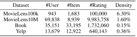
for implicit feedback, we follow BPR (Rendle et al. 2009) to convert rating data into implicit feedback. Particularly, we set ratings greater than 3.5 as positive feedback. Table 2 summarizes the filtered datasets. For each user, we ran-domly sampled 50% ratings as training as the rest as testing. We repeated for five random splits and reported the averaged results.

Table 2: Statistics of datasets

Dataset #User #Item #Rating Density

MovieLens100k 943 1,683 100,000 6.30% MovieLens10M 69,838 8,939 9,983,758 1.60% Book 35,151 33,195 1,732,060 0.15% Yelp 13,679 12,922 640,143 0.36%

Comparison Methods For hashing-based recommender system, we compare ABinCF with 3 very popular and state-of-art methods:DCF, PPH, BCCF. Note that DCF tackles a discrete optimization problem directly which is subject to de-correlated and balanced constraints for seeking compact and informative binary codes for users and items. PPH and BCCF are both two-stage method to learn hash code. BCCF is a Binary Code learning method for Collaborative Filter-ing and PPH is a two-stage Preference PreservFilter-ing HashFilter-ing. However, they haven’t been designed for implicit feedback. For real-based recommender system, we only compare the latest and state-of-art method: IRGAN. It uses gen-erative and discriminative information retrieval models to do recommendation and it is especially designed for im-plicit feedback problems, which outperforms almost other continuous models including BPR (Rendle et al. 2009), LambdaFM (Yuan et al. 2016).

Evaluation Metric We evaluate the recommendation sys-tem performance by a widely used ranking based metric: NDCG(Normalized Discounted Cumulative Gain) and Pre-cision. NDCG is the normalization of DCG(Discounted Cu-mulative Gain) which can measure the ranking quality. Pre-cision is the ratio of the number of relevant results to the total number of results. In our experiment, we predicted the top-K preference items for each user from testing datasets.

Parameter Settings In our experiments, we set β = max(exp(−epoch),0.01) for ABinCF-erf on all datasets andτ = exp(−0.1∗epoch)on MovieLens100K,τ = 0.9

on other datasets for ABinCF-Gn. For all datasets, we setσ

of ABinCF-Gn as 0.01, set the dimension of latent factork

as 16 and setλas0.1/batchsize. We set the sampling tem-perature to 0.2, and the number of generated relevant items to 5 for policy gradient and the number of negative items to the number of positive ones for discriminative learning for IRGAN and ABinCF on all datasets following (Wang et al. 2017).

Besides, for other baselines, we held-out evaluation method on randomly splits of training data to tune the opti-mal hyper-parameters for them by grid search. The settings of them are listed in Table 3.

Table 3: Parameter Settings

DCF BCCF PPH

α β λ λ

MovieLens100k 1 10 0.09 16 MovieLens10M 0.001 10 0.09 16

Book 10 10 0.01 16

Yelp 0.001 10 0.01 8

Comparison with Baselines

Although hashing recommendation has significant advan-tages of time and storage over real-valued recommendation, it often suffers from low recommendation accuracy because binary codes lose a lot of information compared with real-valued codes due to the discrete constraints. ABinCF is pro-posed to improve the recommendation accuracy.

In this part, we will answer the first question at the begin-ning of the experiment section. The recommendation accu-racy comparisons including Precision@10 and NDCG@10 are shown in Table 4, Table 5, Table 6 and Table 7.

Compared with other hash-based recommendation, the performance of ABinCF-Gn far surpasses all other hash al-gorithms including DCF, BCCF and PPH. And ABinCF-erf has huge advantages over other hash-based algorithms on Amazon, Yelp and MovieLens10M dataset while the value of Precision@100 is a little smaller than PPH on Movie-Lens100k. Because Amazon, Yelp and MovieLens10M are sparser than MovieLens100k, so our model based on adver-sarial collaborative filtering can show more advantages on generating high quality negative samples which are signifi-cant in implicit feedback tasks. So ABinCF-erf achieves the best performance about Precision@100 and NDCG@100 on Amazon. ABinCF-Gn has better performance than oth-ers including ABinCF-erf on MovieLens and Yelp be-cause Normal Gumbel-softmax method makes it approxi-mate Bernoulli distribution well. In addition, DCF, BCCF and PPH are designed to make binary codes for explicit rec-ommendation, and BCCF is a two-stage method and PPH is based on quantization method while ABinCF relax sign function directly, so ABinCF has much better results.

Compared with the state-of-art real-valued recommenda-tion algorithm IRGAN, precision loss of ABinCF-erf is less than 30% in almost datasets while the gap between ABinCF-erf and IRGAN is larger than that between ABinCF-Gn and IRGAN. Because IRGAN is real-based method, it obtains more information from real-valued codes. And ABinCF ap-proximates both in sampling of policy gradient and making hash codes, so IRGAN performs better than ours.

The Effectiveness of Normal Gumbel-softmax

Method

We next show the effectiveness of Normal Gumbel-softmax method as follows:

(1)Normal Gumbel-softmax method can approximate Bernoulli distribution greatly. We set τ = 0.001,α = 0, which means 0 and 1 have same probability according to

(6)

Table 4: Item Recommendation Results(MovieLens100k)

Precision@3 Precision@10 Precision@100 NDCG@3 NDCG@10 NDCG@100

IRGAN 0.4396 0.3627 0.1578 0.4542 0.4074 0.4807

DCF 0.0964 0.0962 0.0752 0.1135 0.1058 0.1609

BCCF 0.1336 0.1223 0.0974 0.1331 0.1266 0.2071

PPH 0.1863 0.1779 0.1065 0.1952 0.1893 0.2853

ABinCF-erf 0.2327 0.2005 0.1034 0.2387 0.2204 0.2970

ABinCF-Gn 0.2742 0.2192 0.1129 0.2814 0.2466 0.3244

Table 5: Item Recommendation Results(MovieLens10M)

IRGAN 0.2576 0.2104 0.0972 0.2646 0.2336 0.2683

DCF 0.0589 0.0356 0.0201 0.0748 0.0502 0.0639

BCCF 0.0328 0.0358 0.0330 0.0325 0.0348 0.0521

PPH 0.0418 0.0348 0.0244 0.0492 0.0423 0.0783

ABinCF-erf 01156 0.0759 0.0273 0.1372 0.1025 0.0840

ABinCF-Gn 0.2582 0.2066 0.0590 0.2648 0.2293 0.2043

Table 6: Item Recommendation Results(Amazon)

IRGAN 0.0458 0.0377 0.0194 0.0474 0.0416 0.0629

DCF 0.0113 0.0115 0.0097 0.0109 0.0114 0.0266

BCCF 0.0142 0.0141 0.0111 0.0140 0.0142 0.0280

PPH 0.0065 0.0038 0.0030 0.0065 0.0091 0.0090

ABinCF-erf 0.0334 0.0263 0.0156 0.0351 0.0295 0.0479

ABinCF-Gn 0.0352 0.0274 0.0143 0.0364 0.0307 0.0457

Table 7: Item Recommendation Results(Yelp)

IRGAN 0.0873 0.0705 0.0356 0.0896 0.0800 0.1475

DCF 0.0102 0.0104 0.0095 0.0098 0.0107 0.0325

BCCF 0.0101 0.0094 0.0093 0.0100 0.0100 0.0307

PPH 0.0077 0.0078 0.0068 0.0079 0.0083 0.0240

ABinCF-erf 0.0474 0.0340 0.0218 0.0434 0.0384 0.0831

ABinCF-Gn 0.0510 0.0422 0.0223 0.0520 0.0472 0.0893

and x ∼ N(0,0.01) 1M times respectively and compute G=σ(α−_τx). The value interval ofGis shown in Figure 1. In case ofσ= 1,σ= 0.1orσ= 0.01, it is clear to find that our method can approximate well.

(2)Normal Gumbel-softmax method is more effective than Gumbel noise andG2_{-LSTM noise. We count the number}

of elements in|ui|less than absolute value of Gumbel-based noise and ABinCF-Gn noise at the beginning and the end of the first training on MovieLens100k. The result is shown in Figure 1 where the left part is the beginning of first training and the right part is the end of the first training. If noise is larger than parameters needed updating, it will have a greater impact on the gradient. From Figure 1, noise of Gumbel-based method is too large and ours can update parameters

much more effectively. Therefore, this experiment verifies the analysis in the part of General Gumbel-softmax method.

The Setting of Temperature

In this section, we answer the third question. We show the value of Precision@10 and NDCG@10 via iterations with different ways to set tempera-ture in ABinCF-erf and AbinCF-Gn. In this exper-iment, we set the number of epoch as 15 and the number of iteration within each epoch as 20. We test temperature=exp(−0.01∗epoch), temperature=exp(−0.1∗

epoch), temperature=max(exp(−epoch),0.01) and tem-perature=0.1. We did this experiment in MovieLens100k.

(7)

0.0 0.2 0.4 0.6 0.8 1.0

Value-Range

0 0.2 0.4 0.6

Probability

0.0 0.2 0.4 0.6 0.8 1.0

Value-Range

0 0.15 0.3 0.45

Probability

0.0 0.2 0.4 0.6 0.8 1.0

Value-Range

0 0.15 0.3 0.45

Probability

(a)

Before Training After Training 0

0.2 0.4 0.6 0.8 1

Percentage

Gumbel G2

-LSTM ABinCF-Gn

(b)

Figure 1: (a):The statistics of interval of random variables using the Normal Gumbel-softmax method with different values of

σ. Left.σ= 1.Middle.σ= 0.1.Right.σ= 0.01. (b):The percentage of the absolute value of user latent vectors smaller than the absolute value of stochastic noise by three methods before and after the first training

0 60 120 180 240 300

Iteration

0.12 0.16 0.2 0.24

Precision@10 exp(-0.01*epoch)exp(-0.1*epoch) max(exp(-epoch), 0.01) 0.1

0 60 120 180 240 300

Iteration

0.15 0.18 0.21 0.24

NDCG@10 exp(-0.01*epoch) exp(-0.1*epoch) max(exp(-epoch), 0.01) 0.1

0 60 120 180 240 300

Iteration

0.12 0.16 0.2 0.24

Precision@10 exp(-0.01*epoch)_{exp(-0.1*epoch)}

max(exp(-epoch), 0.01) 0.1

0 60 120 180 240 300

Iteration

0.1 0.15 0.2 0.25 0.3

NDCG@10 exp(-0.01*epoch) exp(-0.1*epoch) max(exp(-epoch), 0.01) 0.1

Figure 2: Left 1.Precision@10 vs Temperature(ABinCF-erf);Left 2.NDCG@10 vs Temperature(ABinCF-erf);Right 1.Preci-sion@10 vs Temperature(ABinCF-Gn);Right 2.NDCG@10 vs Temperature(ABinCF-Gn)

0 2 4 6 8 10

itemNum/million

0 10 20 30 40 50

time/second

hash continuous

0 2 4 6 8 10

itemNum/million

0 5 10 15

memory/kb

×105 hash continuous

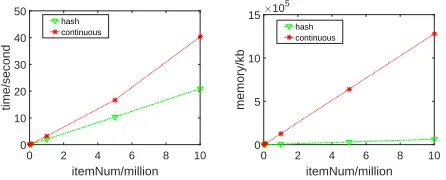
Figure 3: Time and Storage Cost vs Item Size

left figures of Figure 2 shows Precision@10 and NDCG@10 of ABinCF-erf. It is clear to observe that when tempera-ture is set as temperatempera-ture=max(exp(−epoch),0.01), it has much better performance than setting temperature 0.1 be-cause such low temperature at the beginning is hard to train, so our method updating temperature is valid. We also find the green line in the two right ones of Figure 2 representing temperature=0.1achieving the highest results in the first 120 iterations but it drops after. This is because the temperature is too low to update parameters. Besides, the red and blue curves rise during all the training time. Thus we can set tem-perature as a constant a bit larger than 0.1 or set temtem-perature changes with the increase of epoch.

Efficiency Comparison

According to the analysis before, the significant advantage of hashing method of recommendation over real-based rec-ommendation is the efficiency of online recrec-ommendation.

We follow PPH to study the efficiency of hashing-based rec-ommendation on the Amazon dataset. However, the number of candidate items is only 33,195, so it is impossible to test efficiency of recommendation in the case of large size of candidate items. To this end, we assume real-valued item la-tent factors from IRGAN’s generative model following mul-tivariable Gaussian distribution, and then sample latent fac-tors of 10K, 100K, 1M, 5M, and 10M items based on the estimated mean and covariance. Some users’ latent factors from IRGAN’s generative model are used as a query code. Given this synthetic dataset, we compared the efficiency of recommendation and storage cost between real-valued and binary-valued models. The real-valued model directly uses latent factors of the user and items while the binary-valued model exploits the binarzied representation of these latent factors. The effectiveness of hashing-based recommendation compared with real-based recommendation is shown in Fig-ure 3.

Time Complexity The time cost variation over different item sizes is shown in Figure 3. We can conclude that the hashing-based recommendation spends much less time than real-valued recommendation. When the number of users and items becomes much larger which is above millions, the time consuming is extremely huge. Therefore, hashing-based rec-ommendation is much more effective in terms of time than real-based recommendation.

(8)

The storage superiority of hash codes will show more com-pletely when items become larger.

Conclusions

In this paper, we propose an adversarial-based CF hashing framework ABinCF for implicit feedback. By our proposed learning strategy and approximation methods, ABinCF-erf and ABinCF-Gn both outpABinCF-erform the state-of-the-art hashing-based collaborative filtering algorithms and have small accuracy loss compared to real-based algorithm IR-GAN for implict feedback on four public datasets. Our ex-periments also show the proposed ABinCF has great advan-tages in speed of online recommendation and storage. There-fore, it reconciles both effectiveness and efficiency.

Acknowledgements

This research is supported by the National Natural Science Foundation of China (Grant No. 61502077 and 61631005).

References

Allgower, E. L., and Georg, K. 2012. Numerical continuation methods: an introduction, volume 13. Springer Science & Business Media.

Bennett, J.; Lanning, S.; et al. 2007. The netflix prize. In Proceed-ings of KDD cup and workshop, volume 2007, 35. New York, NY, USA.

Cao, Z.; Long, M.; Wang, J.; and Philip, S. Y. 2017. Hashnet: Deep learning to hash by continuation. InICCV, 5609–5618.

Courbariaux, M.; Hubara, I.; Soudry, D.; El-Yaniv, R.; and Bengio, Y. 2016. Binarized neural networks: Training deep neural networks with weights and activations constrained to+ 1 or-1.arXiv preprint arXiv:1602.02830.

Das, A. S.; Datar, M.; Garg, A.; and Rajaram, S. 2007. Google news personalization: scalable online collaborative filtering. In Proceedings of the 16th international conference on World Wide Web, 271–280. ACM.

Goodfellow, I.; Pouget-Abadie, J.; Mirza, M.; Xu, B.; Warde-Farley, D.; Ozair, S.; Courville, A.; and Bengio, Y. 2014. Genera-tive adversarial nets. InAdvances in neural information processing systems, 2672–2680.

H˚astad, J. 2001. Some optimal inapproximability results.Journal of the ACM (JACM)48(4):798–859.

He, X.; He, Z.; Du, X.; and Chua, T.-S. 2018. Adversarial per-sonalized ranking for recommendation. InThe 41st International ACM SIGIR Conference on Research & Development in Informa-tion Retrieval, 355–364. ACM.

Hromkoviˇc, J. 2013.Algorithmics for hard problems: introduction to combinatorial optimization, randomization, approximation, and heuristics. Springer Science & Business Media.

Hu, Y.; Koren, Y.; and Volinsky, C. 2008. Collaborative filtering for implicit feedback datasets. InData Mining, 2008. ICDM’08. Eighth IEEE International Conference on, 263–272. Ieee. Jang, E.; Gu, S.; and Poole, B. 2016. Categorical reparameteriza-tion with gumbel-softmax.arXiv preprint arXiv:1611.01144. Karatzoglou, A.; Smola, A.; and Weimer, M. 2010. Collaborative filtering on a budget. InProceedings of the Thirteenth International Conference on Artificial Intelligence and Statistics, 389–396. Koren, Y., and Bell, R. 2015. Advances in collaborative filtering. InRecommender systems handbook. Springer. 77–118.

Li, Z.; He, D.; Tian, F.; Chen, W.; Qin, T.; Wang, L.; and Liu, T.-Y. 2018. Towards binary-valued gates for robust lstm training. arXiv preprint arXiv:1806.02988.

Liu, X.; He, J.; Deng, C.; and Lang, B. 2014. Collaborative hash-ing. InProceedings of the IEEE conference on computer vision and pattern recognition, 2139–2146.

Maddison, C. J.; Mnih, A.; and Teh, Y. W. 2016. The concrete distribution: A continuous relaxation of discrete random variables. arXiv preprint arXiv:1611.00712.

Muja, M., and Lowe, D. G. 2009. Fast approximate nearest neigh-bors with automatic algorithm configuration. VISAPP (1) 2(331-340):2.

Pan, R.; Zhou, Y.; Cao, B.; Liu, N. N.; Lukose, R.; Scholz, M.; and Yang, Q. 2008. One-class collaborative filtering. InData Mining, 2008. ICDM’08. Eighth IEEE International Conference on, 502– 511. IEEE.

Rendle, S.; Freudenthaler, C.; Gantner, Z.; and Schmidt-Thieme, L. 2009. Bpr: Bayesian personalized ranking from implicit feed-back. InProceedings of the twenty-fifth conference on uncertainty in artificial intelligence, 452–461. AUAI Press.

Royden, H., and Fitzpatrick, P. 1988. Real analysis, 3’rd edition. Song, J. 2017. Binary generative adversarial networks for image retrieval.arXiv preprint arXiv:1708.04150.

Wang, J.; Yu, L.; Zhang, W.; Gong, Y.; Xu, Y.; Wang, B.; Zhang, P.; and Zhang, D. 2017. Irgan: A minimax game for unifying gener-ative and discrimingener-ative information retrieval models. In Proceed-ings of the 40th International ACM SIGIR conference on Research and Development in Information Retrieval, 515–524. ACM. Wang, Q.; Yin, H.; Hu, Z.; Lian, D.; Wang, H.; and Huang, Z. 2018. Neural memory streaming recommender networks with adversarial training. InProceedings of the 24th ACM SIGKDD International Conference on Knowledge Discovery & Data Mining, 2467–2475. ACM.

Wang, J.; Kumar, S.; and Chang, S.-F. 2012. Semi-supervised hash-ing for large-scale search. IEEE Transactions on Pattern Analysis & Machine Intelligence(12):2393–2406.

Williams, R. J. 1992. Simple statistical gradient-following algo-rithms for connectionist reinforcement learning.Machine learning 8(3-4):229–256.

Yuan, F.; Guo, G.; Jose, J. M.; Chen, L.; Yu, H.; and Zhang, W. 2016. Lambdafm: learning optimal ranking with factorization ma-chines using lambda surrogates. InProceedings of the 25th ACM International on Conference on Information and Knowledge Man-agement, 227–236. ACM.

Yuan, F.; Yao, L.; and Benatallah, B. 2018. Adversarial collab-orative auto-encoder for top-n recommendation. arXiv preprint arXiv:1808.05361.

Zhang, Z.; Wang, Q.; Ruan, L.; and Si, L. 2014. Preference pre-serving hashing for efficient recommendation. InProceedings of the 37th international ACM SIGIR conference on Research & de-velopment in information retrieval, 183–192. ACM.

Zhang, H.; Shen, F.; Liu, W.; He, X.; Luan, H.; and Chua, T.-S. 2016. Discrete collaborative filtering. InProceedings of the 39th International ACM SIGIR conference on Research and Develop-ment in Information Retrieval, 325–334. ACM.