The Thirty-Third AAAI Conference on Artificial Intelligence (AAAI-19)
Randomized Strategies for Robust Combinatorial Optimization
∗Yasushi Kawase
Tokyo Institute of TechnologyRIKEN AIP Center [email protected]
Hanna Sumita
Tokyo Metropolitan UniversityAbstract
In this paper, we study the following robust optimization problem. Given an independence system and candidate ob-jective functions, we choose an independent set, and then an adversary chooses one objective function, knowing our choice. The goal is to find a randomized strategy (i.e., a prob-ability distribution over the independent sets) that maximizes the expected objective value in the worst case. This problem is fundamental in wide areas such as artificial intelligence, machine learning, game theory and optimization. To solve the problem, we propose two types of schemes for design-ing approximation algorithms. One scheme is for the case when objective functions are linear. It first finds an approx-imately optimal aggregated strategy and then retrieves a de-sired solution with little loss of the objective value. The ap-proximation ratio depends on a relaxation of an independence system polytope. As applications, we provide approximation algorithms for a knapsack constraint or a matroid intersec-tion by developing appropriate relaxaintersec-tions and retrievals. The other scheme is based on the multiplicative weights update (MWU) method. The direct application of the MWU method does not yield a strict multiplicative approximation algorithm but yield one with an additional additive error term. A key technique to overcome the issue is to introduce a new con-cept called(η, γ)-reductions for objective functions with pa-rametersηandγ. We show that our scheme outputs a nearly
α-approximate solution if there exists anα-approximation al-gorithm for a subproblem defined by(η, γ)-reductions. This improves approximation ratios in previous results. Using our result, we provide approximation algorithms when the objec-tive functions are submodular or correspond to the cardinality robustness for the knapsack problem.
1
Introduction
Optimization under uncertainty about the objective is a fun-damental task in artificial intelligence and machine learn-ing. For example, consider the problem of controlling pan-tilt-zoom cameras to protect against adversarial intru-sions (Krause, Roper, and Golovin 2011). We need to choose where to point the cameras under some scenarios of intru-sions. Thus, we aim to maximize the chance of detecting intrusions in the worst case. See also (Chen et al. 2017) for
∗
A full version appears in (Kawase and Sumita 2018). Copyright c2019, Association for the Advancement of Artificial Intelligence (www.aaai.org). All rights reserved.
another example. Krause, Roper, and Golovin (2011) and Chen et al. (2017) formulated such problems as the follow-ing robust combinatorial optimization problem; given an in-dependence system (E,I)(where I ⊆ 2E) and set func-tionsf1, . . . , fn: 2E → R+, the goal is to find a minimax
randomized strategy pthat maximizes the worst case per-formance, i.e.,mink∈{1,...,n}PX∈IpXfk(X). Throughout this paper, we denote[n] = {1, . . . , n}for a positive inte-ger n. An independence system is a set system generaliz-ing families of knapsack solutions and matroids; we give the formal definition in the preliminaries. The above problem is regarded as the problem of computing thegame valuein a two-person zero-sum game where one player (Algorithm) selects a feasible solution and the other player (Adversary) selects an objective function.
The robust optimization problem has also widespread ap-plication in game theory and combinatorial optimization.
One is the problem of computing theStackelberg equilib-rium of the (zero-sum)security games. This game models the interaction between a systemdefender(Algorithm) and a maliciousattacker(Adversary) to the system. The model and its game-theoretic solution have various applications in the real world (Tambe 2011).
Another application is the problem of maximizing the cardinality robustness for the maximum weight indepen-dent set problem (Hassin and Rubinstein 2002; Fujita, Kobayashi, and Makino 2013; Kakimura and Makino 2013; Matuschke, Skutella, and Soto 2018; Kobayashi and Takazawa 2016). The goal is to choose an independent set of size at mostkwith as large total weight as possible, but the cardinality boundk is not known in advance. We refer this problem to themaximum cardinality robustness prob-lem (MCRP). We can regard MCRP as the game where Al-gorithm chooses an independent setX and then Adversary chooseskknowingX. We will describe details of these ap-plications in the preliminaries.
exponen-tially large cardinality in general, and hence the number of the variables in the LP formulation is exponentially large.
For another way, we can use the multiplicative weights update (MWU) method to solve the problem. The MWU method is an algorithmic technique which maintains a dis-tribution on a certain set of interest and updates it iteratively by multiplying the probability mass of elements by suitably chosen factors based on feedback obtained by running an-other algorithm on the distribution (Kale 2007). MWU is simple but so powerful that it is widely used in game the-ory, machine learning, computational geometry, optimiza-tion, and so on. Freund and Schapire (1999) apply the MWU method to calculate the approximate value of a two-person zero-sum game, and showed that if (i) the set of deter-ministic strategies for Adversary is polynomially sized, and (ii) Algorithm can compute a best response, then MWU gives a polynomial-time algorithm to compute the game value up to an additive error of for any fixed constant
> 0. Krause, Roper, and Golovin (2011) and Chen et al. (2017) extended this result for the case when the algo-rithm can compute only an approximately best response. They provided a polynomial-time algorithm that finds an
α-approximation of the game value up to additive error of
·maxk∈[n], X∈Ifk(X)for any fixed constant >0. This result leads no theoretical guarantee in general because the maximum objective value can be arbitrarily large compared with the optimal value. Moreover, obtaining an (α−0) -approximation solution for a fixed constant 0 > 0 by their algorithms requires pseudo-polynomial time. Recently, Hellerstein, Lidbetter, and Pirutinsky (2018) provided an (α−)-approximation algorithm with the MWU method for the case when the minimizer has exponentially many strate-gies. However, in our problem, it is hard to obtain a similar result by applying their technique.
In this paper, to solve the robust optimization prob-lem, we provide two general schemes based on LP and MWU. As consequences, we develop (approximation) al-gorithms that works when the objective functions and the constraint that defines I belong to well-known classes in combinatorial optimization, such as submodular functions, knapsack/matroid/µ-matroid intersection constraints.
Related workWhile there exist still few papers on random-ized strategies of the robust optimization problems, algo-rithms to find a deterministic strategy have been intensively studied in various setting. See survey papers (Aissi, Bazgan, and Vanderpooten 2009; Kasperski and Zieli´nski 2016) and references therein for details. Adopting a randomized strat-egy provides us two merits: the randomization improves the worst case value dramatically, and the optimal randomized strategy can be found easier than the deterministic one. We will describe these later in the preliminaries.
Since Hassin and Rubinstein (2002) introduced the no-tion of the cardinality robustness, many papers have been investigating the value of the maximum cardinality ro-bustness (Hassin and Rubinstein 2002; Fujita, Kobayashi, and Makino 2013; Kakimura and Makino 2013; Kobayashi and Takazawa 2016; Kakimura, Makino, and Seimi 2012). Kakimura, Makino, and Seimi (2012) proved that the
de-terministic version of MCRP is weakly NP-hard but ad-mits an FPTAS. Matuschke, Skutella, and Soto (2018) intro-duced randomized strategies for the cardinality robustness, and they presented a randomized strategy with (1/ln 4) -robustness for a certain class of independence system. How-ever, they did not consider the computational aspect of the cardinality robustness.
Whenn= 1, the deterministic version of the robust opti-mization problem is exactly the classical optiopti-mization prob-lemmaxX∈If(X). For the monotone submodular function
maximization problem, there exist(1−1/e)-approximation algorithms under a knapsack constraint (Sviridenko 2004) or a matroid constraint (Calinescu et al. 2007; Filmus and Ward 2012), and there exists a 1/(µ+ )-approximation algo-rithm under aµ-matroid intersection constraint for any fixed
>0(Lee, Sviridenko, and Vondr´ak 2010). For the uncon-strained non-monotone submodular function maximization problem, there exists a 1/2-approximation algorithm, and this is best possible (Feige, Mirrokni, and Vondr´ak 2011; Buchbinder et al. 2015). As for the case when the objective function f is linear, the knapsack problem admits an FP-TAS (Kellerer, Mansini, and Speranza 2000).
Main results and technique
LP-based algorithmWe provide a two-step scheme for the case when all the objective functionsf1, . . . , fn are linear. The first step solves the LP that finds an aggregated strat-egy for the original problem, and the second step retrieves a randomized strategy. In the both steps, we make use of a separation problem for the polytope of the feasible re-gion in the LP, which consists of the independence system polytope. We show that if we can solve the separation prob-lem efficiently, then we can also solve the robust optimiza-tion problem efficiently (Theorem 3). Consequently, the ro-bust optimization problem can be solve in polynomial-time whenIcomes from a matroid, a matroid intersection, ors–t
paths. This is a standard application of techniques obtained by Gr¨otschel, Lov´asz, and Schrijver (2012). However, the scheme is not directly available whenIcomes from a knap-sack or aµ-matroid intersection (µ≥3) because the corre-sponding separation problems are NP-hard. A key point to resolve the issue is to use a slight relaxation of the feasible region. We show that if we can efficiently solve the separa-tion problem for the relaxed polytope, then we can know an approximate optimal value (Theorem 4). The most difficult point is the retrieval step, because the LP optimal solution may not belong to the original feasible region. Instead we compute a randomized strategy by slightly shrinking the ag-gregated strategy vector. We prove the approximation ratio of the randomized strategy (Theorem 4). By developing ap-propriate relaxations and retrievals, we show a PTAS and a 2/(eµ)-approximation algorithm for the knapsack constraint and theµ-matroid intersection constraint, respectively.
half-space and a vertex representation of a polytope have different utility, and hence it is important that the LP-based algorithm can deal with both.
MWU-based algorithm We improve the technique of (Krause, Roper, and Golovin 2011; Chen et al. 2017) to ob-tain a better approximation algorithm based on the MWU method. Their algorithm adopts the value offk(X) (k ∈ [n])for update, but this may lead the slow convergence when
fk(X)is too large for somek. In fact, the direct application of the MWU method does not yield a strict multiplicative approximation algorithm but a multiplicative approximation algorithm with an additional additive error term. To over-come this drawback, we make the convergence rate per it-eration faster by introducing a novel concept called(η, γ) -reductionof objective functions (Definition 1). We assume that the algorithm can find anα-best response in the game where objective functions are(η, γ)-reductions of original ones, for anyηand some polynomially boundedγ≤1. We use the procedure as a subroutine. Then we show that by appropriately setting η, for any fixed constant > 0, our scheme gives an(α−)-approximation solution in polyno-mial time with respect tonand1/(Theorem 8). For exam-ple, we give an (η,1/|E|)-reduction for submodular func-tions through submodular minimization. We remark that the support size of the output may be equal to the number of it-erations. Without loss of the objective value, we can find a sparse solution whose support size is at mostnby using LP. The merit of the MWU-based algorithm is applicabil-ity to a wide class of the robust optimization problem. We also demonstrate our scheme for various optimization prob-lems. For any η ≥ 0, we show that a linear function has an (η,1/|E|)-reduction to a linear function, a monotone submodular function has an (η,1)-reduction to a mono-tone submodular function, and a non-monomono-tone submod-ular function has an(η,1/|E|)-reduction to a submodular function. Therefore, we can construct subroutines owing to existing work. Consequently, for the linear case, we obtain an FPTAS subject to the knapsack constraint (Theorem 13) and a 1/(µ−1 + )-approximation algorithm subject to theµ-matroid intersection constraint (Theorem 11). For the monotone submodular case, there exist a (1−1/e −) -approximation algorithm for the knapsack or matroid con-straint (Theorem 9), and a 1/(µ +)-approximation for theµ-matroid intersection constraint (Theorem 10). For the non-monotone submodular case without a constraint, we de-rive a(1/2−)-approximation algorithm (Theorem 12).
Moreover, by applying our MWU-based scheme, we demonstrate an FPTAS for MCRP where I is defined from the knapsack problem (Theorem 14). To construct the subroutine for computing an approximate best re-sponse, we give a gap-preserving reduction of the subprob-lem to maxX∈Iv≤k(X) for anyk, which admits an FP-TAS (Caprara et al. 2000). We also show that MCRP is NP-hard.
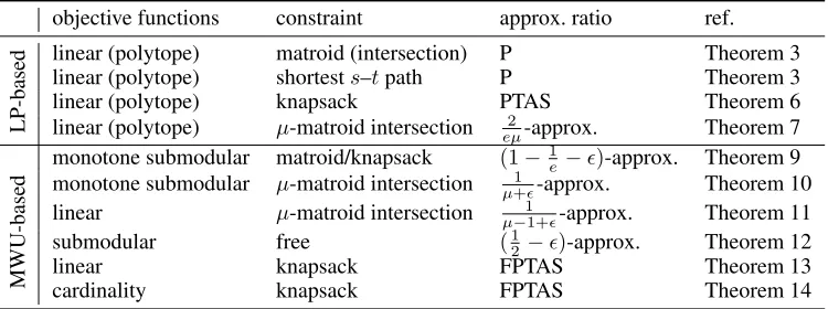
We remark that both schemes produce a randomized strat-egy, but the schemes themselves are deterministic. Our re-sults are summarized in Table 1.
2
Preliminaries
Linear and submodular functionsThroughout this paper, we consider set functionsf withf(∅) = 0. We say that a set functionf: 2E →
Rissubmodulariff(X) +f(Y)≥ f(X∪Y) +f(X ∩Y)holds for allX, Y ⊆E(Fujishige 2005; Krause and Golovin 2014). In particular, a set function
f: 2E →
Ris calledlinear(modular) iff(X) +f(Y) = f(X ∪Y) +f(X ∩Y) holds for all X, Y ⊆ E. A lin-ear function f is represented as f(X) = P
e∈Xwe for some (we)e∈E. A function f is said to be monotone if f(X) ≤ f(Y) for all X ⊆ Y ⊆ E. A linear function
f(X) = P
e∈Xwe is monotone if and only if we ≥ 0 (e∈E).
Independence systemLetEbe a finite ground set. An in-dependence systemis a set system(E,I)with the following properties: (I1)∅ ∈ I, and (I2)X ⊆Y ∈ IimpliesX ∈ I. A set I ⊆ I is said to beindependent, and an inclusion-wise maximal independent set is called abase. The class of independence systems is wide and it includes matroids,µ -matroid intersections, and families of knapsack solutions.
A matroidis an independence system (E,I) satisfying that (I3) if X, Y ∈ I and |X| < |Y| then there exists
e∈Y\Xsuch thatX∪{e} ∈ I. All bases of a matroid have the same cardinality, which is called therankof the matroid and is denoted byρ(I). An example of matroids is a uniform matroid(E,I), whereI = {S ⊆ E | |S| ≤ r}for some
r. Note that the rank of this uniform matroid is r. Given two matroidsM1 = (E,I1)andM2 = (E,I2), the
ma-troid intersectionofM1andM2is defined by(E,I1∩ I2).
Similarly, givenµmatroidsMi = (E,Ii) (i= 1, . . . , µ), theµ-matroid intersection is defined by(E,Tµ
i=1Ii). Given an item set E with sizes(e) and value v(e) for eache∈ E, and the capacityC ∈Z+, theknapsack
prob-lemis to find a subsetXofEthat maximizes the total value
P
e∈Xv(e)subject to a knapsack constraint
P
e∈Xs(e)≤
C. Each subset satisfying the knapsack constraint is called a knapsack solution. LetI = {X | P
e∈Xs(e) ≤ C} be the family of knapsack solutions. Then,(E,I)is an inde-pendence system.
Robust optimization problemLetEbe a finite ground set, and letnbe a positive integer. Let∆(I)and∆ndenote the set of probability distributions over a familyI ⊆2Eand[n], respectively. Given nset functionsf1, . . . , fn: 2E → R+
and an independence system(E,I), our task is to solve
max min k∈[n]
X
X∈I
pX·fk(X) s.t. p∈∆(I). (1)
For eachk∈[n], we denoteXk∗ ∈arg maxX∈Ifk(X)and assume thatfk(Xk∗)>0. We assume that the functions are given by anoracle, i.e., for a givenX ⊆E, we can query an oracle about the valuesf1(X), . . . , fn(X).
By von Neumann’s minimax theorem, it holds that
max
p∈∆(I)kmin∈[n]
X
X∈I
pXfk(X) = min q∈∆n
max
X∈I
X
k∈[n]
qkfk(X). (2)
Table 1: The approximation ratios for robust optimization problems shown in the present paper.
objective functions constraint approx. ratio ref.
LP-based
linear (polytope) matroid (intersection) P Theorem 3 linear (polytope) shortests–tpath P Theorem 3
linear (polytope) knapsack PTAS Theorem 6
linear (polytope) µ-matroid intersection eµ2-approx. Theorem 7
MWU-based
monotone submodular matroid/knapsack (1−1
e−)-approx. Theorem 9 monotone submodular µ-matroid intersection µ+1-approx. Theorem 10 linear µ-matroid intersection µ−11+-approx. Theorem 11
submodular free (12−)-approx. Theorem 12
linear knapsack FPTAS Theorem 13
cardinality knapsack FPTAS Theorem 14
Proposition 1. Let ν∗ denote the optimal value of (1). It holds thatmink∈[n]fk(Xk∗)/n≤ν∗ ≤mink∈[n]fk(Xk∗).
This implies that we can find a1/n-approximate solution by just computingXk∗(k∈[n]).
We describe two merits to adopt a randomized strat-egy rather than a deterministic one for (1). One is that the randomization improves the worst case value dra-matically. Suppose that I = {∅,{a},{b}}, f1(X) =
|X ∩ {a}|, and f2(X) = |X ∩ {b}|. Then, the
maxi-mum worst case value among deterministic strategies is maxX∈Imink∈{1,2}fk(X) = 0, while that for randomized ones is maxp∈∆(I)mink∈{1,2}PX∈IpX·fk(X) = 1/2. The other merit is that the optimal randomized strategy can be found easier. It is known that finding an optimal determin-istic solution is hard even in a simple setting (Aissi, Bazgan, and Vanderpooten 2009; Kasperski and Zieli´nski 2016). In particular, we see in the following that even for an easy case, computing the optimal worst case value among deterministic solutions is strongly NP-hard even to approximate.
Theorem 1. It is NP-hard to compute X ∈ I maxi-mizing mink∈[n]fk(X)even when the objective functions
f1, . . . , fk are linear andI is given by a uniform matroid. Moreover, there exists no approximation algorithm for the problem unless P=NP.
Note that we will show that the randomized version of this problem is polynomial-time solvable (Theorem 3).
Application 1: security gameIn a security game, we are givenntargetsE. The defender selects a set of targetsX ∈ I ⊆2E, and then the attacker selects a facilityi∈ E. The utility of defender isri if i ∈ X andci if i 6∈ X. Then, we can interpret the game as the robust optimization with
fi(X) =ci+Pj∈Xwijwherewij =ri−ciifi=jand 0ifi6=jfori, j∈E. Then the problem of computing the Stackelberg equilibrium is equivalent to (1).
Application 2: MCRP Consider that given an indepen-dence system (E,I) with weights of elements in E, we choose X ∈ I of size at most k with as large total weight as possible, but k is not known in advance. For each X ∈ I, we denote the total weight of thek heav-iest elements in X by v≤k(X). For α ∈ [0,1], an
inde-pendent set X ∈ I is said to be α-robust if v≤k(X) ≥
α · maxY∈Iv≤k(Y) for any k ∈ [n]. Then, MCRP is to find a randomized strategy that maximizes the ro-bustnessα, i.e.,maxp∈∆(I)mink∈[n]PX∈IpX·v≤k(X)/ maxY∈Iv≤k(Y). This is formulated as (1) by setting
fk(X) =v≤k(X)/maxY∈Iv≤k(Y).
3
LP-based Algorithms
In this section, we propose a computation scheme for the robust optimization problem (1) with linear functions
f1, . . . , fn, i.e.,fk(X) =Pe∈Xwke. Here,wke ≥0holds for k ∈ [n] and e ∈ E since we assume fk(X) ≥ 0. A key technique is the separation problem for an indepen-dence system polytope. An independence system polytope of (E,I)is a polytope defined as P(I) = conv{χ(X) | X ∈ I} ⊆[0,1]E, whereχ(X)is a characteristic vector in {0,1}E, i.e.,χ(X)
e = 1if and only ife ∈X. For a prob-ability distributionp∈∆(I), we can get a pointx∈P(I) such thatxe=PX∈I:e∈XpX(e∈E). Then,xe(e∈E) means a probability thateis chosen when we select an inde-pendent set according to the probability distributionp. Con-versely, for any x ∈ P(I), there exists p ∈ ∆(I) such thatP
X∈IpXχ(X) =xby the definition ofP(I). Given
x∈RE, the separation problem forP(I)is to either assert x ∈ P(I)or find a vectordsuch thatd>x < d>y for all
y∈P(I).
The rest of this section is organized as follows. In Sec-tion 3.1, we prove that we can solve (1) in polynomial time if there is a polynomial-time algorithm to solve the separa-tion problem for P(I). In Section 3.2, we tackle the case when it is hard to construct a separation algorithm forP(I). We show that we can obtain an approximation solution when we can slightly relaxP(I). Moreover, we deal with a set-ting that objective functions are given by a polytope in Sec-tion 3.3.
3.1
Basic scheme
We observe that the optimal robust value of (1) is equal to the optimal value of the following linear programming (LP):
max ν s.t. ν≤X e∈E
Lemma 1. Whenf1, . . . , fnare linear, the optimal value of (3)is equal to that of (1).
Thus the optimal solution of (1) is obtained by the follow-ing two-step scheme.
1. compute the optimal solution of LP (3), which we denote as(ν∗, x∗),
2. computep∗∈∆(I)such thatx∗=P
X∈Ip∗Xχ(X). It is trivial that if |I| is bounded by a polynomial in |E| and n, then we can obtain p∗ by replacing x with
P
X∈IpXχ(X) in (3) and solving it. In general, we can solve the two problems in polynomial time by the ellipsoid method when we have a polynomial-time algorithm to solve the separation problem forP(I). This is due to the following theorems given by Gr¨otschel, Lov´asz, and Schrijver (2012). Theorem 2 (Gr¨otschel, Lov´asz, and Schrijver). LetP ⊆ REbe a polytope and suppose that the separation problem forPcan be solved in polynomial time. Then we can solve a linear program overPin polynomial time. In addition, there exists a polynomial time algorithm that, for any vectorx∈ P, computes affinely independent verticesx1, . . . , x` ofP (`≤ |E|+ 1) and positive realsλ1, . . . , λ`withP`i=1λi= 1such thatx=P`
i=1λixi.
Therefore, we have the following general result.
Theorem 3. If f1, . . . , fn are linear and there is a polynomial-time algorithm to solve the separation problem forP(I), then we can solve the linear robust optimization problem(1)in polynomial time.
Hence, there exists a polynomial-time algorithm for (1) when I is a matroid (intersection) or the set ofs–tpaths, because a matroid (intersection) polytope and the dominant of ans–tpath polytope admit a polynomial-time separation algorithm.
3.2
Relaxation of the polytope
We present an approximation scheme for the case when the separation problem for P(I) is hard to solve. Recall that
fk(X) =Pe∈Xwkewherewke≥0fork∈[n]ande∈E. We modify the basic scheme as follows. First, instead of solving the separation problem forP(I), we solve the one for a relaxation of P(I). For a polytope P and a positive number(1≥)α >0, we denoteαP ={αx |x∈P}. We call a polytopePˆ(I) ⊆ [0,1]E α-relaxation of P(I)if it holds thatαPˆ(I)⊆P(I)⊆Pˆ(I). Then we solve
maxx∈Pˆ(I)mink∈[n]Pe∈Ewkexe (4) instead of LP (3), and obtain an optimal solutionxˆ.
Next, we compute a convex combination of xˆ using
χ(X) (X ∈ I). Here, if xˆ ∈ Pˆ(I) is the optimal solu-tion for (4), thenαxˆ ∈P(I)is anα-approximate solution of LP (3), because
max x∈P(I)kmin∈[n]
X
e∈E
wkexe≤ max x∈Pˆ(I)
min k∈[n]
X
e∈E
wkexe
= min k∈[n]
X
e∈E
wkexˆe= 1
α·kmin∈[n]
X
e∈E
wke(αˆxe).
As αxˆ ∈ P(I), there exists p ∈ ∆(I)such that αxˆ =
P
X∈IpXχ(X). However, the retrieval of such a prob-ability distribution may be computationally hard, because the separation problem for P(I)is hard to solve. Hence, we relax the problem and compute p∗ ∈ ∆(I)such that
βxˆ ≤P
X∈Ip∗Xχ(X), where(α≥)β >0. Then,p∗is a
β-approximate solution ofmaxp∈∆(I)mink∈[n]
P
X∈Ip∗X·
fk(X), because
max p∈∆(I)
min k∈[n]
X
X∈I
pX·fk(X)≤ min k∈[n]
X
e∈E
wkexˆe
≤ 1 β ·kmin∈[n]
X
X∈I
p∗X·fk(X).
Thus the basic scheme is modified as the following ap-proximation scheme:
1. compute the optimal solutionxˆ∈Pˆ(I)for LP (4),
2. computep∗ ∈∆(I)such thatβ·xˆe ≤PX∈I:e∈Xp
∗
X for eache∈E.
Theorem 4. Suppose that f1, . . . , fn are linear. If there exists a polynomial-time algorithm to solve the separation problem for an α-relaxation Pˆ(I) of P(I), then an α -approximation of the optimal value of (1) is computed in time. In addition, if there exists a polynomial-time algorithm to find p ∈ ∆(I) such that β · xˆe ≤
P
X∈I:e∈XpX for anyx ∈ Pˆ(I), then a β-approximate solution of (1)is found in polynomial-time.
We remark that we can combine the result in Section 3.3 with this theorem.
In the following, we apply Theorem 4 to two important cases whenIis defined from a knapsack constraint or aµ -matroid intersection. For this end, we develop appropriately relaxations ofP(I)and retrieval procedures forp∗.
Relaxation of a knapsack polytope Let E be a set of items with sizes(e)for eache∈E. Without loss of general-ity, we assume that a knapsack capacity is one, ands(e)≤1 for alle∈E. LetIbe a family of knapsack solutions, i.e., I ={X ⊆E|P
e∈Xs(e)≤1}.
It is known thatP(I)admits apolynomial size relaxation scheme, i.e., there exists a(1−)-relaxation ofP(I)through a linear program of polynomial size for a fixed >0. Theorem 5 (Bienstock). Let 0 < ≤ 1. There ex-ist a polytope P(I) and its extended formulation with
O(−1n1+d1/e)variables andO(−1n2+d1/e)constraints
such that(1−)P(I)⊆P(I)⊆P(I).
Thus, the optimal solution xˆ to maxx∈P(I)mink∈[n] P
e∈Ewkexecan be computed in polynomial time. The re-maining task is to computep∗∈∆(I)such that(1−)·xˆe≤
P
X∈I:e∈Xp∗X for eache ∈ E. We give an algorithm for this task.
Lemma 2. There exists a polynomial-time algorithm that computesp∗∈∆(I)such that(1−)·xˆe≤PX∈I:e∈Xp∗X for eache∈E.
Finally, we remark that the existence of a fully polyno-mial size relaxation scheme (FPSRS)forP(I)is open (Bi-enstock 2008). The existence of an FPSRS leads an FPTAS to compute the optimal value of the linear robust optimiza-tion problem (1) subject to a knapsack constraint.
Relaxation of aµ-matroid intersection polytope Let us consider the case whereIis defined from aµ-matroid inter-section. It is NP-hard to maximize a linear function subject to aµ-matroid intersection constraint ifµ ≥ 3(Garey and Johnson 1979). Hence, it is also NP-hard to solve the linear robust optimization subject to aµ-matroid intersection con-straint ifµ≥3. Fori = 1, . . . , µ, let(E,Ii)be a matroid whose rank function isρi. Let(E,I) = (E,T
i∈[µ]Ii). We definePˆ(I) =T
i∈[µ]P(Ii). We see thatPˆ(I)is a(1/µ) -relaxation ofP(I).
Lemma 3. µ1Pˆ(I)⊆P(I)⊆Pˆ(I).
As we can solve the separation problem for Pˆ(I) in strongly polynomial time (Cunningham 1984), we can ob-tain an optimal solutionxˆ ∈ Pˆ(I)for the relaxed problem maxx∈Pˆ(I)Pe∈Ew(e)xe. Since ˆx/µ ∈ P(I), the value
P
e∈Ew(e)ˆxe/µis aµ-approximation of the optimal value. To obtain aµ-approximate solution, we need to compute
p∗ ∈ ∆(I) such that xˆe/µ ≤ PX∈I:e∈Xp
∗
X for each
e ∈ E. Unfortunately, it seems hard to obtain such a dis-tribution. With the aid of the contention resolution (CR) scheme (Chekuri, Vondr´ak, and Zenklusen 2014), we can computep∗∈∆(I)such that(2/eµ)·xˆe≤PX∈I:e∈Xp∗X for eache ∈ E. We describe its procedure in the full ver-sion (Kawase and Sumita 2018). We can summarize our re-sult as follows.
Theorem 7. We can compute aµ-approximate value of the linear robust optimization problem subject to aµ-matroid intersection in polynomial time. Moreover, we can imple-ment a procedure that efficiently outputs an independent set according to the distribution of a2/(eµ)-approximate solu-tion.
3.3
Linear functions in a polytope
We consider the following variant of (1). Instead ofn func-tionsf1, . . . , fn, suppose that we are given a set of functions
F =
(
f
f({e}) =we(∀e∈E),
Aw+Bψ≤c, w≥0,
ψ≥0
)
for someA ∈Rm×|E|,B ∈Rm×d, andc ∈Rm. Now, we aim to solve
maxp∈∆(I)minf∈FPX∈IpXf(X). (5) Note that for linear functionsf1, . . . , fn, (1) is equivalent to
(5) in which
F= conv{f1, . . . , fn}
=
f
f({e}) =we(e∈E),
we=Pk∈[n]qkfk({e}),
P
k∈[n]qk = 1, w, q≥0
.
We observe that (5) is equal to maxx∈P(I)min{x>w |
Aw+Bψ≤c, w≥0, ψ≥0}by using a similar argument to Lemma 1. The LP duality implies thatmin{x>w|Aw+
Bψ≤c, w≥0, ψ≥0}= max{c>y|A>y≥x, B>y≥
0, y ≥0}. Thus the optimal value of (5) is equal to that of the LP maxx∈P(I)maxy:A>y=x, B>y≥0, y≥0Pi∈[m]biyi. Hence, Theorem 2 implies that if the separation problem for
P(I)can be solved in polynomial time, then we can solve (5) in polynomial time.
4
MWU-based Algorithm
In this section, we present an algorithm based on the MWU method (Arora, Hazan, and Kale 2012). This algorithm is applicable to general cases. We assume thatfk(X)≥0for anyk∈[n]andX ∈ I.
We describe the idea of our algorithm. Let us focus on the right hand side of the minimax relation (2). We define weightsωkfor each functionfk, and iteratively update them. Intuitively, a function with a larger weight is likely to be cho-sen with higher probability. At the first round, all functions have the same weights. At each roundt, we set a probability
qk (k ∈[n])thatfk is chosen by normalizing the weights. Then we compute an (approximate) optimal solutionX(t)of
maxX∈IPk∈[n]qk·fk(X). To minimize the right hand side of (2), the probabilityqkfor a functionfkwith a larger value
fk(X)should be decreased. Thus we update the weights ac-cording tofk(X). We repeat this procedure, and set a ran-domized strategyp∈∆(I)according toX(t)’s.
Krause, Roper, and Golovin (2011) and Chen et al. (2017) proposed the above algorithm whenf1, . . . , fnare functions with range [0,1]. They proved that if there exists an α -approximation algorithm to maxX∈IPk∈[n]qkfk(X) for any q ∈ ∆n, then the approximation ratio is α− for any fixed constant > 0. This implies an approximation ratio ofα−·maxk∈[n], X∈Ifk(X)/ν∗ whenf1, . . . , fn are functions with rangeR+, whereν∗is the optimal value
of (1). Here, maxk∈[n], X∈Ifk(X)/ν∗ could be large in general. To remove this term from the approximation ra-tio, we introduce a novel concept of function transforma-tion. We improve the existing algorithms (Chen et al. 2017; Krause, Roper, and Golovin 2011) with this concept, and show a stronger result later in Theorem 8.
Definition 1. For positive reals η and γ (≤ 1), we call a function g is an (η, γ)-reduction of f if (i) g(X) ≤
min{f(X), η}and (ii)g(X)≤γ·ηimpliesg(X) =f(X). Intuitively, the condition (i) is useful for speeding up MWU and the condition (ii) is important for the purpose that the optimal value does not change significantly.
We fix a parameter γ > 0, where 1/γ is bounded by polynomial. The smallerγis, the wider the class of(η, γ) -reduction of f is. We set another parameter η later. We denote (η, γ)-reduction of f1, . . . , fn by f1η, . . . , fnη, re-spectively. In what follows, suppose that we have an α -approximation algorithm to
maxX∈IPk∈[n]qkfkη(X) (6) for anyq ∈ ∆n andη ∈ R+∪ {∞}. In our proposed
ηis, the faster our algorithm converges. However, the limit outcome of our algorithm asTgoes to infinity moves over a little from the optimal solution. We overcome this issue by settingηto an appropriate value.
Our algorithm is summarized in Algorithm 1. Note that
fk∞ = fk (k ∈ [n]). We remark that when the parameter
γis small, there may exist a better approximation algorithm for (6), but the running time of Algorithm 1 becomes longer.
Algorithm 1:MWU for the robust optimization
input : positive realsη,δ(≤1/2), and an integerT
output: randomized strategyp∗∈∆(I)
1 Letω(1)k ←1for eachk∈[n]; 2 fort= 1, . . . , T do
3 q(kt)←ωk(t)/Pk∈[n]ω(kt)for eachk∈[n]; 4 letX(t)be anα-approximate solution of
maxX∈IPk∈[n]q (t)
k ·f η k(X);
5 ωk(t+1)←ωk(t)(1−δ)f η k(X
(t))/η
for eachk∈[n];
6 returnp∗∈∆(I)such that
p∗X=|{t∈ {1, . . . , T} |X(t)=X}|/T;
The main result of this section is stated below.
Theorem 8. If there exists anα-approximation algorithm to solve(6) for anyq ∈ ∆n andη ∈ R+∪ {∞}, then
Algo-rithm 1 is an(α−)-approximation algorithm to the robust optimization problem(1) for any fixed > 0. In addition, the running time of Algorithm 1 isO(nα2ln3γnθ), whereθ is
the running time of theα-approximation algorithm to(6).
To show this, we use the following lemma, which can be proved by standard analysis of the MWU method (see, e.g., Arora, Hazan, and Kale (2012)). In the following, we denote byν∗the optimal value of (1).
Lemma 4. For anyδ∈(0,1/2], it holds that
T X
t=1
X
k∈[n]
q(kt)·fkη(X(t))≤ ηlnn
δ + (1 +δ)·kmin∈[n] T X
t=1
fkη(X(t)).
Next, we see that the optimal value of (1) forf1, . . . , fn and the one forf1η, . . . , fη
nare close ifηis a large number. Lemma 5. Ifη≥ n
δγ ·ν
∗, we have
ν∗≥ min q∈∆n
max X∈I
X
k∈[n]
qk·fkη(X)≥(1−δ)ν∗.
By Lemmas 4 and 5, we have the following lemma, which implies Theorem 8.
Lemma 6. For any fixed >0, the outputp∗of Algorithm 1 is an(α−)-approximate solution of (1)when we setT =
dn2lnn
αδ3γ e, n2
αδγν
∗≥η≥ n δγν
∗, andδ= min{/3,1/2}.
As applications of Theorem 8, we can obtain the follow-ing theorems.
When f1, . . . , fn are monotone submodular, f η k(X) = min{fk(X), η} is an (η,1)-reduction of fk, andfkη is a
monotone submodular function (Lov´asz 1983; Fujito 2000). Thus, P
k∈[n]qkf
η
k(X) is monotone submodular for any
q ∈ ∆n. Because there exist(1−1/e)-approximation al-gorithms for maximizing a monotone submodular function under a knapsack constraint (Sviridenko 2004) and under a matroid constraint (Calinescu et al. 2007; Filmus and Ward 2012), we can obtain the following theorems.
Theorem 9. For any positive real > 0, there exists a
(1−1/e−)-approximation algorithm for the robust op-timization problem(1)whenf1, . . . , fnare monotone sub-modular andI is given by a knapsack constraint or a ma-troid.
Theorem 10. For any fixed positive real >0, there exists a
1/(µ+)-approximation algorithm for the robust optimiza-tion problem(1)whenf1, . . . , fnare monotone submodular andIis given by aµ-matroid intersection.
A monotone linear maximization subject to a µ-matroid intersection can be viewed as a monotone submodular max-imization subject to a(µ−1)-matroid intersection. Thus, we also obtain the following theorem.
Theorem 11. For any fixed positive real > 0, there ex-ists a1/(µ−1 +)for the robust optimization problem(1) whenf1, . . . , fn are monotone linear andI is given by a
µ-matroid intersection.
When f1, . . . , fn are (non-monotone) submodular, min{fk, η}may not a submodular function. In this case, we definefkη(X) = min{f(Z) +η· |X−Z|/|E| |Z ⊆X}. Then,fkη is an(η,1/|E|)-reduction offk. Sincefkη(X)is a submodular function (Fujishige 2005), we can evaluate the valuefkη(X)in strongly polynomial time by a submodular function minimization algorithm. Thus, the following theorem holds.
Theorem 12. For any fixed positive real > 0, there ex-ists a(1/2−)-approximation algorithm for the robust op-timization problem(1)whenf1, . . . , fnare submodular and I = 2E.
When fk(X) = Pe∈Xwke for each k ∈ [n], where
wke ≥ 0 ande ∈ E,fkη(X) = Pe∈Xmin{wke, η/|E|} is an(η,1/|E|)-reduction of fk. In addition, we can con-struct an FPTAS to computemaxX∈IPk∈[n]qkf
η k(X)for anyq∈∆n.
Theorem 13. There exists an FPTAS for the robust opti-mization problem(1)whenf1, . . . , fn are monotone linear andIis given by a knapsack constraint.
Finally, we apply Theorem 8 to MCRP for the knap-sack problem. Recall that the objective functions are given as fk(X) = v≤k(X)/maxY∈Iv≤k(Y) fori ∈ [k]. Note that the evaluation of fk(X) for a given solution X is already NP-hard. We provide an FPTAS to evaluate the value of fk’s and then we develop an FPTAS to solve maxX∈IPk∈[n]qkf
η
k(X). Therefore, we can obtain the following theorem.
Acknowledgments
The first author is supported by JSPS KAKENHI Grant Number JP16K16005 and JST ACT-I Grant Number JP-MJPR17U7. The second author is supported by JST ERATO Grant Number JPMJER1201, Japan, and JSPS KAKENHI Grant Number JP17K12646.
References
Aissi, H.; Bazgan, C.; and Vanderpooten, D. 2009. Min– max and min–max regret versions of combinatorial opti-mization problems: A survey. EJOR197(2):427–438.
Arora, S.; Hazan, E.; and Kale, S. 2012. The multiplicative weights update method: a meta-algorithm and applications. Theor. Comp.8(1):121–164.
Bienstock, D. 2008. Approximate formulations for 0–1 knapsack sets. Oper. Res. Let.36(3):317–320.
Bowles, S. 2009. Microeconomics: behavior, institutions, and evolution. Princeton University Press.
Buchbinder, N.; Feldman, M.; Naor, J. S.; and Schwartz, R. 2015. A tight linear time (1/2)-approximation for uncon-strained submodular maximization. SICOMP44(5):1384– 1402.
Calinescu, G.; Chekuri, C.; P´al, M.; and Vondr´ak, J. 2007. Maximizing a submodular set function subject to a matroid constraint. InIPCO, volume 7, 182–196. Springer.
Caprara, A.; Kellerer, H.; Pferschy, U.; and Pisinger, D. 2000. Approximation algorithms for knapsack problems with cardinality constraints. EJOR123(2):333–345.
Chekuri, C.; Vondr´ak, J.; and Zenklusen, R. 2014. Submod-ular function maximization via the multilinear relaxation and contention resolution schemes. SICOMP43(6):1831– 1879.
Chen, R. S.; Lucier, B.; Singer, Y.; and Syrgkanis, V. 2017. Robust optimization for non-convex objectives. InAdvances in Neural Information Processing Systems, 4708–4717.
Cunningham, W. H. 1984. Testing membership in matroid polyhedra. JCTB36(2):161–188.
Feige, U.; Mirrokni, V. S.; and Vondr´ak, J. 2011. Max-imizing non-monotone submodular functions. SICOMP 40(4):1133–1153.
Filmus, Y., and Ward, J. 2012. A tight combinatorial al-gorithm for submodular maximization subject to a matroid constraint. InProc. of FOCS, 659–668. IEEE.
Freund, Y., and Schapire, R. E. 1999. Adaptive game play-ing usplay-ing multiplicative weights. GEB29(1-2):79–103.
Fujishige, S. 2005.Submodular functions and optimization, volume 58. Elsevier.
Fujita, R.; Kobayashi, Y.; and Makino, K. 2013. Ro-bust matchings and matroid intersections.SIDMA27:1234– 1256.
Fujito, T. 2000. Approximation algorithms for submodular set cover with applications. IEICE Transactions on Infor-mation and Systems83(3):480–487.
Garey, M. R., and Johnson, D. S. 1979. Computers and Intractability: A Guide to the Theory of NP-Completeness. Freeman New York.
Gr¨otschel, M.; Lov´asz, L.; and Schrijver, A. 2012. Geomet-ric algorithms and combinatorial optimization, volume 2. Springer Science & Business Media.
Hassin, R., and Rubinstein, S. 2002. Robust matchings. SIDMA15(4):530–537.
Hellerstein, L.; Lidbetter, T.; and Pirutinsky, D. 2018. Solv-ing zero-sum games usSolv-ing best response oracles with appli-cations to search games. arXiv:1704.02657v4.
Kakimura, N., and Makino, K. 2013. Robust independence systems. SIDMA27(3):1257–1273.
Kakimura, N.; Makino, K.; and Seimi, K. 2012. Computing knapsack solutions with cardinality robustness. Japan Jour-nal of Industrial and Applied Mathematics29(3):469–483. Kale, S. 2007. Efficient algorithms using the multiplica-tive weights update method. Ph.D. Dissertation, Princeton University.
Kasperski, A., and Zieli´nski, P. 2016. Robust Discrete Op-timization Under Discrete and Interval Uncertainty: A Sur-vey. Springer International Publishing. 113–143.
Kawase, Y., and Sumita, H. 2018. Randomized strategies for robust combinatorial optimization. arXiv:1805.07809. Kellerer, H.; Mansini, R.; and Speranza, M. G. 2000. Two linear approximation algorithms for the subset-sum prob-lem. EJOR120:289–296.
Kobayashi, Y., and Takazawa, K. 2016. Randomized strate-gies for cardinality robustness in the knapsack problem. Theoretical Computer Science.
Krause, A., and Golovin, D. 2014. Submodular function maximization. InIn Tractability: Practical Approaches to Hard Problems (to appear). Cambridge University Press. Krause, A.; Roper, A.; and Golovin, D. 2011. Random-ized sensing in adversarial environments. InProc. of IJCAI, volume 22, 2133–2139.
Lee, J.; Sviridenko, M.; and Vondr´ak, J. 2010. Submodu-lar maximization over multiple matroids via generalized ex-change properties.Math. Oper. Res.35(4):795–806. Lov´asz, L. 1983. Submodular functions and convexity. In Mathematical Programming The State of the Art. Springer. 235–257.
Matuschke, J.; Skutella, M.; and Soto, J. A. 2018. Robust randomized matchings. Math. Oper. Res.43(2):675–692.
Nisan, N.; Roughgarden, T.; Tardos, ´E.; and Vazirani, V. V. 2007. Algorithmic Game Theory. Cambridge University Press.
Sviridenko, M. 2004. A note on maximizing a submodular set function subject to a knapsack constraint.Oper. Res. Let. 32(1):41–43.