Probabilistic Line Searches for Stochastic Optimization
Maren Mahsereci [email protected]
Philipp Hennig [email protected]
Max Planck Institute for Intelligent Systems Max-Planck-Ring 4, 72076 T¨ubingen, Germany
Editor:Mark Schmidt
Abstract
In deterministic optimization, line searches are a standard tool ensuring stability and efficiency. Where only stochastic gradients are available, no direct equivalent has so far been formulated, because uncertain gradients do not allow for a strict sequence of decisions collapsing the search space. We construct a probabilistic line search by combining the structure of existing deterministic methods with notions from Bayesian optimization. Our method retains a Gaussian process surrogate of the univariate optimization objective, and uses a probabilistic belief over the Wolfe conditions to monitor the descent. The algorithm has very low computational cost, and no user-controlled parameters. Experiments show that it effectively removes the need to define a learning rate for stochastic gradient descent. Keywords: stochastic optimization, learning rates, line searches, Gaussian processes, Bayesian optimization
1. Introduction
This work substantially extends the work of Mahsereci and Hennig (2015) published at NIPS 2015. Stochastic gradient descent (sgd, Robbins and Monro, 1951) is currently the standard in machine learning for the optimization of highly multivariate functions if their gradient is corrupted by noise. This includes the online or mini-batch training of neural networks, logistic regression (Zhang, 2004; Bottou, 2010) and variational models (e.g. Hoffman et al., 2013; Hensman et al., 2012; Broderick et al., 2013). In all these cases, noisy gradients arise because an exchangeable loss-functionL(x) of the optimization parametersx∈RD, across
a large dataset{di}i=1...,M, is evaluated only on a subset{dj}j=1,...,m:
L(x) := 1 M
M X
i=1
`(x, di)≈
1 m
m X
j=1
`(x, dj) =: ˆL(x) mM. (1)
If the indices j are i.i.d. draws from [1, M], by the Central Limit Theorem, the error ˆ
L(x)− L(x) is unbiased and approximately normal distributed. Despite its popularity and its low cost per step, sgdhas well-known deficiencies that can make it inefficient, or at least tedious to use in practice. Two main issues are that, first, the gradient itself, even without noise, is not the optimal search direction; and second, sgdrequires a step size (learning rate) that has drastic effect on the algorithm’s efficiency, is often difficult to choose well, and virtually never optimal for each individual descent step. The former issue, adapting the search direction, has been addressed by many authors (see George and Powell, 2006, for
c
an overview). Existing approaches range from lightweight ‘diagonal preconditioning’ like Adam(Kingma and Ba, 2014),AdaGrad(Duchi et al., 2011), and ‘stochastic meta-descent’ (Schraudolph, 1999), to empirical estimates for the natural gradient (Amari et al., 2000) or
the Newton direction (Roux and Fitzgibbon, 2010), to problem-specific algorithms (Rajesh et al., 2013), and more elaborate estimates of the Newton direction (Hennig, 2013). Most of these algorithms also include an auxiliary adaptive effect on the learning rate. Schaul et al. (2013) provided an estimation method to explicitly adapt the learning rate from one gradient
descent step to another. Several very recent works have proposed the use of reinforcement learning and ‘learning-to-learn’ approaches for parameter adaption (Andrychowicz et al., 2016; Hansen, 2016; Li and Malik, 2016). Mostly these methods are designed to work well on a specified subset of optimization problems, which they are also trained on; they thus need to be re-learned for differing objectives. The corresponding algorithms are usually orders of magnitude more expensive than the low-level black box proposed here, and often require a classic optimizer (e.g sgd) to tune their internal hyper-parameters.
None of the mentioned algorithms change the size of the current descent step. Accu-mulating statistics across steps in this fashion requires some conservatism: If the step size is initially too large, or grows too fast, sgd can become unstable and ‘explode’, because individual steps are not checked for robustness at the time they are taken.
0 0.5 1 1.5
−2 0 2 4
À Á
Â
¹
distancetin line search direction
f
0(t
)
5.5 6 6.5
À
Á Â
¹
f
(
t
)
Figure 1: Sketch: The task of a classic line search is to tune the step taken by an optimization algorithm along a univariate search direction. The search starts at the endpoint À of the previous line search, at t = 0. The upper plot shows function values, the lower plot corresponding gradients. A sequence of ex-trapolation stepsÁ,Âfinds a point of positive gradient atÂ. It is followed by interpolation steps until an acceptable point ¹ is found. Points of insufficient decrease, above the line f(0) +c1tf0(0) (white area in upper plot) are excluded by the Armijo condition W-I, while points of steep negative gradient (white area in lower plot) are excluded by the curvature condition W-II (the strong extension of the Wolfe conditions also excludes the light green area in the lower plot). Point¹is the first to fulfill both conditions, and is thus accepted.
methods (Nocedal and Wright, 1999,§3).1 In the noise-free case, line searches are considered a solved problem (Nocedal and Wright, 1999,§3). But the methods used in deterministic optimization are not stable to noise. They are easily fooled by even small disturbances, either becoming overly conservative or failing altogether. The reason for this brittleness is that existing line searches take a sequence of hard decisions to shrink or shift the search space. This yields efficiency, but breaks hard in the presence of noise. Section 3 constructs a probabilistic line search for noisy objectives, stabilizing optimization methods like the works cited above. As line searches only change the length, not the direction of a step, they could be used in combination with the algorithms adaptingsgd’s direction, cited above. In this paper we focus on parameter tuning of the sgdalgorithm and leave other search directions to future work.
2. Connections
2.1 Deterministic Line Searches
There is a host of existing line search variants (Nocedal and Wright, 1999, §3). In essence, though, these methods explore a univariate domain ‘to the right’ of a starting point, until an ‘acceptable’ point is reached (Figure 1). More precisely, consider the problem of minimizing
L(x) :RD_R, with access to∇L(x) :R
D
_R
D. At iterationi, some ‘outer loop’ chooses,
at locationxi, a search directionsi∈RD (e.g. by thebfgs-rule, or simplysi =−∇L(xi) for
gradient descent). It willnot be assumed that si has unit norm. The line search operates
along the univariate domain x(t) = xi +tsi for t ∈ R+. Along this direction it collects scalar function values and projected gradients that will be denoted f(t) = L(x(t)) and f0(t) = s|i∇L(x(t))∈R. Most line searches involve an initial extrapolation phase to find
a pointtr with f0(tr)>0. This is followed by a search in [0, tr], by interval nesting or by
interpolation of the collected function and gradient values, e.g. with cubic splines.2 2.1.1 The Wolfe Conditions for Termination
As the line search is only an auxiliary step within a larger iteration, it need not find an exact root off0; it suffices to find a point ‘sufficiently’ close to a minimum. The Wolfe conditions (Wolfe, 1969) are a widely accepted formalization of this notion; they considert acceptable
if it fulfills
f(t)≤f(0) +c1tf0(0) (W-I) and f0(t)≥c2f0(0) (W-II), (2) using two constants 0≤c1 < c2 ≤1 chosen by the designer of the line search, not the user. W-I is theArmijo orsufficient decrease condition (Armijo, 1966). It encodes that acceptable functions values should lie below a linear extrapolation line of slope c1f0(0). W-II is the curvature condition, demanding a decrease in slope. The choice c1 = 0 accepts any value below f(0), while c1 = 1 rejects all points for convex functions. For the curvature condition,
1. In these algorithms, another task of the line search is to guarantee certain properties of the surrounding
estimation rule. Inbfgs, e.g., it ensures positive definiteness of the estimate. This aspect will not feature
here.
2. This is the strategy inminimize.mby C. Rasmussen, which provided a model for our implementation. At
−10 1
ρ
(
t
)
0 0.5 1
0 0.2 0.4 0.6 0.8 1
distancetin line search direction
p
W
olfe
(
t
) weak
strong 0
1
pb
(
t
)
0 1
pa
(
t
)
ÀÁ Â Ä Ï Ã
5.5 6 6.5
f
(
t
)
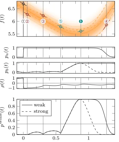
Figure 2: Sketch of a probabilistic line search. As in Fig. 1, the algorithm performs extrapo-lation (Á,Â,Ã) and interpolation (Ä,Ï), but receives unreliable, noisy function and gradient values. These are used to construct agpposterior (top. solid pos-terior mean, thin lines at 2 standard de-viations, local pdf marginal as shading, three dashed sample paths). This implies a bivariate Gaussian belief (§3.3) over the validity of the weak Wolfe conditions (middle three plots. pa(t) is the marginal
for W-I, pb(t) for W-II, ρ(t) their
corre-lation). Points are considered acceptable if their joint probability pWolfe(t) (bot-tom) is above a threshold (gray). An ap-proximation (§3.3.1) to the strong Wolfe conditions is shown dashed.
c2 = 0 only accepts points withf0(t)≥0; whilec2 = 1 accepts any point of greater slope than f0(0). W-I and W-II are known as theweak form of the Wolfe conditions. Thestrong form replaces W-II with|f0(t)| ≤c2|f0(0)|. This guards against accepting points of low function value but large positive gradient. Figure 1 shows a conceptual sketch illustrating the typical process of a line search, and the weak and strong Wolfe conditions. The exposition in§3.3 will initially focus on the weak conditions, which can be precisely modeled probabilistically. Section 3.3.1 then adds an approximate treatment of the strong form.
2.2 Bayesian Optimization
3. A Probabilistic Line Search
We now consider minimizingf(t) = ˆL(x(t)) from Eq. 1. That is, the algorithm can access only noisy function values and gradients yt, yt0 at locationt, with Gaussian likelihood
p(yt, yt0|f) =N
yt
y0t
;
f(t) f0(t)
,
σ2f 0 0 σf20
. (3)
The Gaussian form is supported by the Central Limit argument at Eq. 1. The function value yt and the gradient yt0 are assumed independent for simplicity; see §3.4 and Appendix A
regarding estimation of the variancesσf2, σf20, and some further notes on the independence assumption ofy and y0. Each evaluation of f(t) uses a newly drawn mini-batch.
Our algorithm is modeled after the classic line search routineminimize.m2 and translates each of its building blocks one-by-one to the language of probability. The following table illustrates these four ingredients of the probabilistic line search and their corresponding classic parts.
building block classic probabilistic
1)1D surrogate for objectivef(t)
piecewise cubic splines gpwhere the mean are piece-wise cubic splines
2) candidate selection onelocal minimizer of cubic splines xor extrapolation
local minimizers of cubic splines and extrapolation
3) choice of best candidate ——— bo acquisition function
4)acceptance criterion classic Wolfe conditions prob. Wolfe conditions
The table already motivates certain design choices, for example the particular choice of the gp-surrogate for f(t), which strongly resembles the classic design. Probabilistic line searches operate in the same scheme as classic ones: 1) they construct a surrogate for the underlying 1D-function 2) they select candidates for evaluation which can interpolate between datapoints or extrapolate 3) a heuristic chooses among the candidate locations and the function is evaluated there 4) the evaluated points are checked for Wolfe-acceptance. The following sections introduce all of these building blocks with greater detail: A robust yet lightweight Gaussian process surrogate on f(t) facilitating analytic optimization (§3.1); a simple Bayesian optimization objective for exploration (§3.2); and a probabilistic formulation of the Wolfe conditions as a termination criterion (§3.3). Appendix D contains a detailed pseudocode of the probabilistic line search; Algorithm 1 very roughly sketches the structure of the probabilistic line search and highlights its essential ingredients.
3.1 Lightweight Gaussian Process Surrogate
We model information about the objective in a probability measure p(f). There are two requirements on such a measure: First, it must be robust to irregularity (low and high variability) of the objective. And second, it must allow analytic computation of discrete candidate points for evaluation, because a line search should not call yet another optimization subroutine itself. Both requirements are fulfilled by a once-integrated Wiener process, i.e. a zero-mean Gaussian process prior p(f) =GP(f; 0, k) with covariance function
k(t, t0) =θ21/3min3(˜t,˜t0) +1/2|t−t0|min2(˜t,˜t0)
Algorithm 1 probLineSearchSketch(f,y0,y00,σf0,σf00) GP ^initGP(y0,y00,σf0,σf00)
T, Y, Y0^initStorage(0, y0,y00) . for observed points
t^1 .scaled position of initial candidate
while budget not used and no Wolfe-point found do
[y, y0]^f(t) . evaluate objective
T, Y, Y0^updateStorage(t,y,y0) GP^updateGP(t,y,y0)
PWolfe^probWolfe(T,GP) . compute Wolfe probability at points inT
if any PWolfe above Wolfe thresholdcW then return Wolfe-point
else
Tcand^computeCandidates(GP) .positions of new candidates EI^expectedImprovement(Tcand,GP)
P W ^probWolfe(Tcand,GP)
t^ where (P W EI) is maximal .find best candidate among Tcand
end if end while
return observed point inT with lowestgpmean since no Wolfe-point found
Here ˜t:=t+τ and ˜t0:=t0+τ denote a shift by a constantτ >0. This ensures this kernel is positive semi-definite, the precise value τ is irrelevant as the algorithm only considers positive values of t(our implementation uses τ = 10). See §3.4 regarding the scale θ2. With the likelihood of Eq. 3, this prior gives rise to a gpposterior whose mean function is a cubic spline3 (Wahba, 1990). We note in passing that regression on f andf0 fromN observations of pairs (yt, yt0) can be formulated as a filter (S¨arkk¨a, 2013) and thus performed in O(N)
time. However, since a line search typically collects<10 data points, generic gpinference, using a Gram matrix, has virtually the same, low cost.
Because Gaussian measures are closed under linear maps (Papoulis, 1991, §10), Eq. 4 implies a Wiener process (linear spline) model onf0:
p(f;f0) =GP
f f0
;
0 0
,
k k∂ k
∂ ∂ ∂k
, (5)
3. Eq. 4 can be generalized to the ‘natural spline’, removing the need for the constantτ (Rasmussen and
Williams, 2006,§6.3.1). However, this notion is ill-defined in the case of a single observation, as in the
0 1 2 3 4 −1
−0.5 0 0.5
t
f
(
t
)
0 1 2 3 4
t
Figure 3: Integrated Wiener process: gp marginal posterior of function values; posterior mean in solid orange and, two standard deviations in thinner solid orange, local pdf marginal as shading; function value observations as gray circles (corresponding gradients not shown). Classic interpolation by piecewise cubic spline in dark blue. Left: observations are exact; the mean of thegp and the cubic spline interpolator of a classic line search coincide. Right: same observations with additive Gaussian noise (error-bars indicate ± 1 standard deviations); noise free interpolator in dashed gray for comparison. The classic interpolator in dark blue, which exactly matches the observations, becomes unreliable; the gp reacts robustly to noisy observations; thegp-mean still consists of piecewise cubic splines.
with (using the indicator function I(x) = 1 if x, else 0)
k∂tt0 := ∂k(t, t 0)
∂t0 =θ 2
I(t < t0)
˜ t2
2 +I(t≥t 0)
˜ t˜t0−˜t0
2 2
k
∂
tt0 := ∂k(t, t
0)
∂t =θ
2
I(t0 < t)
˜ t02
2 +I(t 0 ≥t)
˜ tt˜0−˜t
2 2 (6) k ∂ ∂
tt0 := ∂
2k(t, t0) ∂t0∂t =θ
2min(˜t,˜t0).
Given a set of evaluations (t,y,y0) (vectors, with elements ti, yti, y0ti) with independent likelihood 3, the posterior p(f|y,y0) is agp with posterior mean functionµand covariance function ˜k as follows:
µ(t) µ0(t)
=
ktt k∂tt k
∂
tt ∂ ∂k tt
ktt+σf2I k∂tt k
∂
tt ∂ ∂k tt+σf20I
−1
| {z }
=:g|(t)
y y0 " ˜
k(t, t0) k˜∂(t, t0) ˜k
∂ (t0, t) ∂ ∂˜k (t, t0)
#
=
ktt0 k∂tt0 k
∂
t0t ∂ ∂k tt0
−g|(t)
ktt0 k∂tt0 k
∂
t0t ∂ ∂k tt0
(7)
The posterior marginal variance will be denoted by V(t) = ˜k(t, t). To see thatµis indeed
derivatives4, because k
∂2
tt0 := ∂
2k(t, t0) ∂t2 =θ
2
I(t≤t0) ∂ k
3
tt0 := ∂
3k(t, t0) ∂t3 =θ
2
I(t≤t0)(t0−t)
k
∂2 ∂
tt0 := ∂
4k(t, t0) ∂t2∂t0 =−θ
2
I(t≤t0) ∂ k
3 ∂
tt0 := ∂
4k(t, t0)
∂t3∂t0 = 0. (8)
This piecewise cubic form of µ is crucial for our purposes: having collectedN values off andf0, respectively, all local minima ofµcan be found analytically inO(N) time in a single sweep through the ‘cells’ ti−1< t < ti,i= 1, . . . , N (here t0= 0 denotes the start location, where (y0, y00) are ‘inherited’ from the preceding line search. For typical line searchesN <10, c.f.§4. In each cell,µ(t) is a cubic polynomial with at most one minimum in the cell, found by an inexpensive quadratic computation from the three scalars µ0(ti), µ00(ti), µ000(ti). This
is in contrast to other gpregression models—for example the one arising from a squared exponential kernel—which give more involved posterior means whose local minima can be found only approximately. Another advantage of the cubic spline interpolant is that it does not assume the existence of higher derivatives (in contrast to the Gaussian kernel, for example), and thus reacts robustly to irregularities in the objective. In our algorithm, after each evaluation of (yN, yN0 ), we use this property to compute a short list ofcandidates
for the next evaluation, consisting of the≤N local minimizers of µ(t) and one additional extrapolation node attmax+α, wheretmax is the currently largest evaluated t, andα is an extrapolation step size starting at α= 1 and doubled after each extrapolation step.5
A conceptual (rather than algorithmic) motivation for using the integrated Wiener process as surrogate for the objective, as well as for the described candidate selection, are classic line searches. There, the 1D-objective is modeled by piecewise cubic interpolations between neighboring datapoints. In a sense, this is a non-parametric approach, since a new spline is defined, when a datapoint is added. Classic line searches always only deal with one spline at a time, since they are able to collapse all other parts of the search space. Indeed, for noise free observations, the mean of the posteriorgp is identical to the classic cubic interpolations, and thus candidate locations are identical as well; this is illustrated in Figure 3. The non-parametric approach also prevents issues of over-constrained surrogates for more than two datapoints. For example, unless the objective is a perfect cubic function, it is impossible to fit a parametric third order polynomial to it, for more than two noise free observations. All other variability in the objective would need to be explained away by artificially introducing noise on the observations. An integrated Wiener process very naturally extends its complexity with each newly added datapoint without being overly assertive – the encoded assumption is that the objective hasat least one derivative (which is also observed in this case).
4. There is no well-defined probabilistic belief overf00and higher derivatives—sample paths of the Wiener
process are almost surely non-differentiable almost everywhere (Adler, 1981,§2.2). Butµ(t) is always
a member of the reproducing kernel Hilbert space induced byk, thus piecewise cubic (Rasmussen and
Williams, 2006,§6.1).
5. For the integrated Wiener process and heteroscedastic noise, the variancealwaysattains its maximum
0 0.5 1 1.5 2 2.5 3 3.5 4 0
0.2 0.4 0.6 0.8 1
←uEI·pWolfe
uEI
↓
pWolfe
↓
step sizet uEI
·
p
W
olfe
←local minimum extrapolation→
−1 0 1
f
0
−2 −1 0
f
Figure 4: Candidate selection by Bayesian optimization. Top: gp marginal posterior of function values. Posterior mean in solid orange and, two standard deviations in thinner solid orange, local pdf marginal as shading. The red and the blue point are evaluations of the objective function, collected by the line search. Middle: gpmarginal posterior of corresponding gradients. Colors same as in top plot. In all three plots the locations of thetwo candidate points (§3.1) are indicated as vertical dark red lines. The left one at abouttcand1 ≈1.54 is a local minimum of the posterior mean in between the red and blue point (the mean of the gradient belief (solid orange, middle plot) crosses through zero here). The right one at tcand2 = 4 is a candidate for extrapolation. Bottom: Decision criterion in arbitrary scale: The expected improvementuEI (Eq. 9) is shown in dashed light blue, the Wolfe probabilitypWolfe (Eq. 14 and Eq. 16) in light red and their decisive product in solid dark blue. For illustrative purposes all criteria are plotted for the whole t-space. In practice solely the values at tcand1 andtcand2 are computed, compared, and the candidate with the higher value ofuEI·pWolfe is chosen for evaluation. In this example this would be the candidate attcand1 .
3.2 Choosing Among Candidates
0 1 2 −1
0 1
pWolfe=0.68
0 1 2
−1 0 1
pWolfe=0.08
0 1 2
−1 0 1
pWolfe=0.00
W-I I W-I ←accepted −1 0 1 f 0
0 0.5 1 1.5 2 2.5 3 3.5 4
−2 −1 0
f
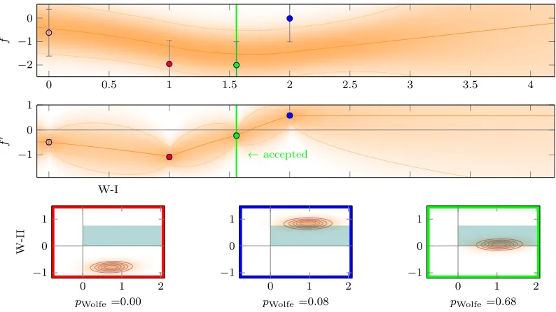
Figure 5: Acceptance procedure. Top and middle: plot and colors as in Figure 4 with an additional ‘green’ observation. Bottom: Implied bivariate Gaussian belief over the validity of the Wolfe conditions (Eq. 11) at the red, blue and green point respectively. Points are considered acceptable if their Wolfe probability pWolfet is above a thresholdcW = 0.3; this means that at least 30% of the orange 2D
Gauss density must cover greenish shaded area. Only the green point fulfills this condition and is therefore accepted.
0 0.5 1 1.5 0 1 t-constraining p W olfe ( t )
−0.2 0 0.2
f
(
t
)
σf = 0.0028
σf0= 0.0049
0 2 4
0 1 t-extrapolation −2 0 2
σf = 0.28
σf0 = 0.0049
0 0.5 1 1.5 0
1
t-interpolation −0.2
0 0.2
σf = 0.082
σf0= 0.014
0 0.5 1 1.5 0
1
t-immediate accept −0.5
0 0.5
σf = 0.17
σf0= 0.012
0 0.5 1 1.5 0
1
t-high noise interpolation −0.2
0 0.2
σf= 0.24
σf0= 0.011
are observed locations),
uEI(t) =Ep(ft|y,y0)[min{0, η−f(t)}] = η−µ(t)
2 1 + erf
η−µ(t)
p
2V(t) !
+
r V(t)
2π exp
−(η−µ(t))
2 2V(t)
. (9)
The next evaluation point is chosen as the candidate maximizing the product of Eq. 9 and Wolfe probability pWolfe, which is derived in the following section. The intuition is that pWolfe precisely encodes properties of desired points, but has poor exploration properties;uEI has better exploration properties, but lacks the information that we are seeking a point with low curvature;uEI thus puts weight on (by W-II) clearly ruled out points. An illustration of the candidate proposal and selection is shown in Figure 4.
In principle other acquisition functions (e.g. the upper-confidence bound, gp-ucb (Srinivas et al., 2010)) are possible, which might have a stronger explorative behavior; we opted for uEI since exploration is less crucial for line searches than for general bo and some (e.g. gp-ucb) had one additional parameter to tune. We tracked the sample efficiency ofuEI instead and it was very good (low); the experimental Subsection 4.3 contains further comments and experiments on the alternative choices ofuEI andpWolfe as standalone acquisition functions; they performed equally well (in terms of loss and sample efficiency) to their product on the tested setups.
3.3 Probabilistic Wolfe Conditions for Termination
The key observation for a probabilistic extension of the Wolfe conditions W-I and W-II is that they are positivity constraints on two variables at, bt that are both linear projections of
the (jointly Gaussian) variablesf andf0:
at bt =
1 c1t −1 0 0 −c2 0 1
f(0) f0(0) f(t) f0(t)
≥0. (10)
The gpof Eq. (5) on f thus implies, at each value of t, a bivariate Gaussian distribution
p(at, bt) =N at bt ;
mat mbt
,
Ctaa Ctab Ctba Ctbb
, (11)
with mat =µ(0)−µ(t) +c1tµ0(0)
mbt =µ0(t)−c2µ0(0) (12)
and Ctaa = ˜k00+ (c1t)2∂ ∂k˜00+ ˜ktt+ 2[c1t(˜k∂00−∂k˜0t)−k0˜ t]
Ctbb=c22∂ ∂˜k00−2c2∂ ∂k˜0t+ ˜∂ ∂ktt
Ctab=Ctba=−c2(˜k00∂ +c1t∂ ∂˜k00) +c2∂˜k0t+ ˜∂kt0+c1t∂ ∂˜k 0t−˜ktt∂.
(13)
The quadrant probability pWolfet =p(at>0∧bt>0) for the Wolfe conditions to hold, is an
integral over a bivariate normal probability,
pWolfet =
Z ∞
−√mat Caat
Z ∞
−√mbt Cbbt N a b ; 0 0 ,
1 ρt
ρt 1
with correlation coefficient ρt=Ctab/ q
CtaaCtbb. It can be computed efficiently (Drezner and Wesolowsky, 1990), using readily available code.6 The line search computes this probability for all evaluation nodes, after each evaluation. If any of the nodes fulfills the Wolfe conditions with pWolfet > cW, greater than some threshold 0 < cW ≤ 1, it is accepted and returned.
If several nodes simultaneously fulfill this requirement, the most recently evaluated node is returned; there are additional safeguards for cases where e.g. no Wolfe-point can be found, which can be deduced from the pseudo-code in Appendix D; they are similar to standard safeguards of classic line search routines (e.g. returning the node of lowest mean). Section 3.4.1 below motivates fixing cW = 0.3. The acceptance procedure is illustrated in
Figure 5.
3.3.1 Approximation for Strong Conditions:
As noted in Section 2.1.1, deterministic optimizers tend to use the strong Wolfe conditions, which use |f0(0)| and |f0(t)|. A precise extension of these conditions to the probabilistic setting is numerically taxing, because the distribution over|f0|is a non-centralχ-distribution, requiring customized computations. However, a straightforward variation to 14 captures the spirit of the strong Wolfe conditions that large positive derivatives should not be accepted: Assuming f0(0)<0 (i.e. that the search direction is a descent direction), the strong second Wolfe condition can be written exactly as
0≤bt=f0(t)−c2f0(0)≤ −2c2f0(0). (15)
The value −2c2f0(0) is bounded to 95% confidence by
−2c2f0(0).2c2(|µ0(0)|+ 2
p
V0(0)) =: ¯b. (16)
Hence, an approximation to the strong Wolfe conditions can be reached by replacing the
infinite upper integration limit on b in Eq. 14 with (¯b−mbt)/
q
Ctbb. The effect of this adaptation, which adds no overhead to the computation, is shown in Figure 2 as a dashed line.
3.4 Eliminating Hyper-parameters
As a black-box inner loop, the line search should not require any tuning by the user. The preceding section introduced six so-far undefined parameters: c1, c2, cW, θ, σf, σf0. We will now show that c1, c2, cW, can be fixed by hard design decisions: θ can be eliminated by
standardizing the optimization objective within the line search; and the noise levels can be estimated at runtime with low overhead for finite-sum objectives of the form in Eq. 1. The result is a parameter-free algorithm that effectively removes the one most problematic parameter from sgd—the learning rate.
3.4.1 Design Parameters c1, c2, cW
Our algorithm inherits the Wolfe thresholdsc1 andc2 from its deterministic sibling. We set c1 = 0.05 andc2= 0.5. This is a standard setting that yields a ‘lenient’ line search, i.e. one
that accepts most descent points. The rationale is that the stochastic aspect of sgdis not always problematic, but can also be helpful through a kind of ‘annealing’ effect.
The acceptance threshold cW is a new design parameter arising only in the probabilistic
setting. We fix it tocW = 0.3. To motivate this value, first note that in the noise-free limit,
all values 0< cW <1 are equivalent, becausepWolfe then switches discretely between 0 and
1 upon observation of the function. A back-of-the-envelope computation, assuming only two evaluations at t= 0 and t=t1 and the same fixed noise level on f and f0 (which then cancels out), shows that function values barely fulfilling the conditions, i.e.at1 =bt1 = 0, can havepWolfe∼0.2 while function values atat1 =bt1 =−for_0 with ‘unlucky’ evaluations (both function and gradient values one standard-deviation from true value) can achieve pWolfe ∼0.4. The choicecW = 0.3 balances the two competing desiderata for precision and
recall. Empirically (Fig. 6), we rarely observed values of pWolfe close to this threshold. Even at high evaluation noise, a function evaluation typically either clearly rules out the Wolfe conditions, or lifts pWolfe well above the threshold. A more in-depth analysis of c1,c2, and cW is done in the experimental Section 4.2.1.
3.4.2 Scale θ
The parameter θ of Eq. 4 simply scales the prior variance. It can be eliminated by scaling the optimization objective: We set θ = 1 and scale yi^(yi−y0)/|y00|, yi0^y
0 i/|y0
0| within the code of the line search. This gives y(0) = 0 and y0(0) = −1, and typically ensures the objective ranges in the single digits across 0< t <10, where most line searches take place. The division by |y00|causes a non-Gaussian disturbance, but this does not seem to have notable empirical effect.
3.4.3 Noise Scales σf, σf0
The likelihood 3 requires standard deviations for the noise on both function values (σf)
and gradients (σf0). One could attempt to learn these across several line searches; but the resulting estimator would be biased. In exchangeable models as captured by Eq. 1, however, the variance of the loss and its gradient can be estimated locally and unbiased, directly for the mini-batch, at low computational overhead—an approach already advocated by Schaul et al. (2013). We collect the empirical statistics
ˆ
S(x) := 1 m
m X
j
`2(x, yj), and ∇ˆS(x) :=
1 m
m X
j
∇`(x, yj)2 (17)
(where 2 denotes the element-wise square) and estimate, at the beginning of a line search from xk,
σ2f = 1 m−1
ˆ
S(xk)−Lˆ(xk)2
and σf20 =si 2|
1 m−1
ˆ
∇S(xk)−(∇Lˆ(xk))2
. (18)
examples N-I and N-II of the experimental Section 4, the additional steps added only ∼1% cost overhead to the evaluation of the loss. This is rather at the lower end for these models; A more general statement about memory and time requirements for neural networks can be found in Sections 3.6 and 3.7. Estimating noise separately for each input dimension captures the often inhomogeneous structure among gradient elements, and its effect on the noise along the projected direction. For example, in multi-layer models, gradient noise is typically higher on weights between the input and first hidden layer, hence line searches along the corresponding directions are noisier than those along directions affecting higher-level weights.
3.4.4 Propagating Step Sizes Between Line Searches
As will be demonstrated in §4, the line search can find good step sizes even if the length of the directionsi is mis-scaled. Since such scale issues typically persist over time, it would be
wasteful to have the algorithm re-fit a good scale in each line search. Instead, we propagate step lengths from one iteration of the search to another: We set the initial search direction tos0=−α0∇Lˆ(x0) with some initial learning rateα0. Then, after each line search ending at xi = xi−1+t∗si, the next search direction is set to si+1 = −αext·t∗α0∇Lˆ(xi) (with
αext = 1.3). Thus, the next line search starts its extrapolation at 1.3 times the step size of its predecessor (Section 4.2.2 for details).
3.5 Relation to Bayesian Optimization and Noise-Free Limit
a Wolfe-point, they do not need to explore the parameter space of possible step sizes to that extend; crucial features are rather the possibility to explore somewhat larger steps than previous ones (which is done by extrapolation-candidates), and likewise to shorted steps (which is done by interpolation-candidates).
In the limit of noise free observed gradients and function values (σf = σf0 = 0) the probabilistic line search behaves like its classic parent, except for very slight variations in the candidate choice (building block 3): Thegp-mean reverts to the classic interpolator; all candidate locations are thus identical, but the probabilistic line search might propose a second option, since (even if there is a local minimizer) italways also proposes an extrapolation candidate. This is illustrated in the following table.
building block classic probabilistic (noise free)
1)1D surrogate for objectivef(t)
piecewise cubic splines gp-mean identical to classic interpolator
2) candidate selection local minimizer of cubic splines xor extrapolation
local minimizer of cubic splines or extrapolation
3) choice of best candidate ——— bo acquisition function
4)acceptance criterion classic Wolfe conditions pWolfe identical to classic Wolfe conditions
3.6 Computational Time Overhead
The line search routine itself has little memory and time overhead; most importantly it is independent of the dimensionality of the optimization problem. After every call of the objective function, the gp (§3.1) needs to be updated which, at most, is at the cost of inverting a 2N ×2N-matrix, where N usually is equal to 1,2, or 3 but never > 10. In addition, the bivariate normal integral pWolfet of Eq. 14 needs to be computed at most N times. On a laptop, one evaluation ofpWolfet costs about 100 microseconds. For the choice among proposed candidates (§3.2), again at most N, for each, we need to evaluate pWolfet and uEI(t) (Eq. 9) where the latter comes at the expense of evaluating two error functions. Since all of these computations have a fixed cost (in total some milliseconds on a laptop), the relative overhead becomes less the more expensive the evaluation of ∇Lˆ(x).
The largest overhead actually lies outside of the actual line search routine. In case the noise levelsσf and σf0 are not known, we need to estimate them. The approach we took is described in Section 3.4.3 where the variance of∇Lˆis estimated using the sample variance of the mini-batch, each time the objective function is called. Since in this formulation the variance estimation is about half as expensive as one backward pass of the net, the time overhead depends on the relative cost of the feed forward and backward passes (Balles et al., 2017). If forward and backward pass are the same cost, the most straightforward implementation of the variance estimation would make each function call <1.3 times as expensive. This is anupper bound and the actual cost is usually lower.7 At the same time though, all exploratory experiments which very considerably increase the time spend when
using sgdwith a hand tuned learning rate schedule need not be performed anymore. In Section 4.1 we will also see that sgd using the probabilistic line search often needs less function evaluations to converge, which might lead to overall faster convergence in wall clock time than classic sgdin a single run.
3.7 Memory Requirement
Vanilla sgd, at all times, keeps around the current optimization parameters x∈RD and the
gradient vector∇Lˆ(x)∈RD. In addition to this, the probabilistic line search needs to store
the estimated gradient variances Σ0(x) = (1−m)−1( ˆ∇S(x)− ∇Lˆ(x)2) (Eq. 18) of same size. The memory requirement of sgd+probLSis thus comparable toAdaGrador Adam. If combined with a search direction other than sgd always one additional vector of sizeD needs to be stored.
4. Experiments
This section reports on an extensive set of experiments to characterise and test the line search. The overall evidence from these tests is that the line search performs well and is relatively insensitive to the choice of its internal hyper-parameters as well the mini-batch size. We performed experiments on two multi-layer perceptrons N-I and N-II; both were trained on two well known datasets MNIST and CIFAR-10.
• N-I: fully connected net with 1 hidden layer and 800 hidden units + biases, and 10 output units, sigmoidal activation functions and a cross entropy loss. Structure without biases: 784-800-10. Many authors used similar nets and reported performances.8
• N-II: fully connected net with 3 hidden layers and 10 output units, tanh-activation functions and a squared loss. Structure without biases: 784-1000-500-250-10. Similar nets were also used for example in Martens (2010) and Sutskever et al. (2013).
• MNIST (LeCun et al., 1998): multi-class classification task with 10 classes: hand-written digits in gray-scale of size 28×28 (numbers ‘0’ to ’9’); training set size 60 000, test set size 10 000.
• CIFAR-10 (Krizhevsky and Hinton, 2009): multi-class classification task with 10 classes: color images of natural objects (horse, dog, frog,. . . ) of size 32×32; training set size 50 000, test set size 10 000; like other authors, we only used the “batch 1” sub-set of CIFAR-10 containing 10 000 training examples.
In addition we train logistic regressors with sigmoidal output (N-III) on the following binary classification tasks:
• Wisconsin Breast Cancer Dataset (WDBC) (Wolberg et al., 2011): binary classification of tumors as either ‘malignant’ or ‘benign’. The set consist of 569 examples of which we used 169 to monitor generalization performing; thus 400 remain for the training set; 30 features describe for example radius, area, symmetry, et cetera. In comparison
to the other datasets and networks, this yields a very low dimensional optimization problem with only 30 (+1 bias) input parameters as well as just a small number of datapoints.
• GISETTE (Guyon et al., 2005): binary classification of the handwritten digits ‘4’ and ‘9’. The original 28×28 images are taken from the MNIST datset; then the feature set was expanded and consists of the original normalized pixels, plus a randomly selected subset of products of pairs of features, which are slightly biased towards the upper part of the image; in total there are 5000 features, instead of 784 as in the original MNIST. The size of the training set and test set is 6000 and 1000 respectively.
• EPSILON: synthetic dataset from the PASCAL Challenge 2008 for binary classification. It consists of 400 000 training set datapoint and 100 000 test set datapoints, each having 2000 features.
In the text and figures,sgdusing the probabilistic line search will occasionally be denoted as sgd+probLS. Section 4.1 contains experiments on the sensitivity to varying gradient noise levels (mini-batch sizes) performed on both multi-layer perceptrons N-I and N-II, as well as on the logistic regressor N-III. Section 4.2 discusses sensitivity to the hyper-parameters choices introduced in Section 3.4 and Section 4.3 contains additional diagnostics on step size statistics. Each single experiment was performed 10 times with different random seeds that determined the starting weights and the mini-batch selection and seeds were shared across all experiments. We report all results of the 10 instances as well as means and standard deviations.
4.1 Varying Mini-batch Sizes
The noise level of the gradient estimate ∇Lˆ(x) and the loss ˆL(x) is determined by the mini-batch size m and ultimately there should exist an optimal m that maximizes the optimizer’s performance in wall-clock-time. In practice of course the cost of computing
∇Lˆ(x) and ˆL(x) is not necessarily linear in m since it is upper bounded by the memory capacity of the hardware used. We assume here that the mini-batch size is chosen by the user; thus we test the line search with the default hyper-parameter setting (see Sections 3.4 and 4.2) on four different mini-batch sizes:
• m= 10,100,200 and 1000 (for MNIST, CIFAR-10, and EPSILON)
• m= 10,50,100, and 400 (for WDBC and GISETTE)
which correspond to increasing signal-to-noise ratios. Since the training set of WDBC only consists of 400 datapoints, the run with the larges mini-batch size of 400 in fact runs full-batch gradient descent on WDBC; this is not a problem, since—as discussed above—the probabilistic line search can also handle noise free observations.9 We compare to sgd-runs using a fixed step size (which is typical for these architectures) and an annealed step size with annealing schedule αt=α0/t. Because annealed step sizes performed much worse than
9. Since the dataset sizeM of WDBC is very small, we used the factor(M−m)/(mM)instead of1/mto scale
the sample variances of Eq. 17. The former encodes sampling mini-batchesBwith replacement, the latter
−4 −2
m:100
−4 −2
m:200
−4 −2
m:1000
−4 −2 −3
−2 −1 0
log learning rate
log
test
and
train
set
error
m:10
0 1 2 3 4
0 1 2 3 4
0 1 2 3 4
−3 −2 −1 0
log
train
set
er
ror
0 1 2 3 4
0 1 2 3 4
−1 0
# function evaluations in 104
log
test
set
erro
r
0 1 2 3 4
0 1 2 3 4 0 1 2 3 4
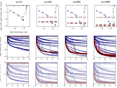
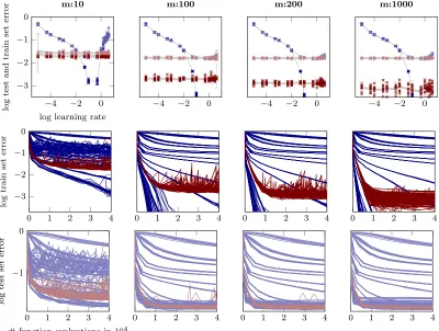
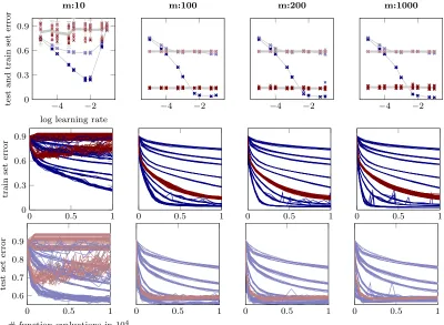
Figure 7: Performance of N-II on MNIST forvarying mini-batch sizes. Top: final logarithmic test set and train set error after 40 000 function evaluations of training versus a large range of learning rates each for 10 different initializations. sgd-runs with fixed learning rates are shown in light blue (test set) and dark blue (train set); sgd+probLS-runs in light red (test set) and dark red (train set); means and two standard deviations for each of the 10 runs in gray. Columns from left to right refer to different mini-batch sizesm of 10, 100, 200 and 1000 which correspond to decreasing relative noise in the gradient observations. Not surprisingly the performance ofsgd-runs with a fixed step size are very sensitive to the choice of this step size. sgdusing the probabilistic line search adapts initially mis-scaled step sizes and performs well across the whole range of initial learning rates. Middle and bottom: Evolution of the logarithmic test and train set error respectively for allsgd-runs andsgd+probLS-runs versus # function evaluations (colors as in top plot). For mini-batch sizes ofm= 100,200 and 1000all instances ofsgdusing the probabilistic line search reach the same best test set error. Similarly a good train set error is reached very fast bysgd+probLS. Only very few instances of sgdwith a fixed learning rate reach a better train set error (and this advantage usually does not translate to test set error). For very small mini-batch sizes (m= 10, first column) the line search performs poorly on this architecture, most
sgd+fixed step size, we will only report on the latter results in the plots.10 Since classic sgd without the line search needs a hand crafted learning rate we search on exhaustive logarithmic grids of
αsgdN-I = [10−5,5·10−5,10−4,5·10−4,10−3,5·10−3,10−2,5·10−2,10−1,5·10−1] αN-IIsgd = [αN-Isgd, 1.0, 1.5, 2.0, 2.5, 3.0, 3.5, 4.0]
αN-IIIsgd = [10−8,10−7,10−6,10−5,10−4,10−3,10−2,10−1,100,101,102].
We run 10 different initialization for each learning rate, each mini-batch size and each net and dataset combination (10·4·(2·10 + 2·17 + 3·11) = 3480 runs in total) for a large enough budget to reach convergence; and report all numbers. Then we perform the same experiments using the same seeds and setups withsgdusing the probabilistic line search and compare the results. Forsgd+probLS,αsgd is the initial learning rate which is used
in the very first step. After that, the line search automatically adapts the learning rate, and shows no significant sensitivity to its initialization.
Results of N-I and N-II on both, MNIST and CIFAR-10 are shown in Figures 7, 14, 15, and 16; results of N-III on WDBC, GISETTE and EPSILON are shown in Figures 18, 17, and 19 respectively. All instances (sgd and sgd+probLS) get the same computational budget (number of mini-batch evaluations) and not the same number of optimization steps. The latter would favour the probabilistic line search since, on average, a bit more than one mini-batch is evaluated per step. Likewise, all plots show performance measure versus the number of mini-batch evaluations, which is proportional to the computational cost.
All plots show similar results: While classicsgdis sensitive to the learning rate choice, the line search-controlled sgdperforms as good, close to, or sometimes even better than the (in practice unknown) optimal classicsgdinstance. In Figure 7, for example,sgd+probLS con-verges much faster to a good test set error than the best classic sgd instance. In all experiments, across a reasonable range of mini-batch sizes m and of initial αsgd values, the line search quickly identified good step sizesαt, stabilized the training, and progressed
efficiently, reaching test set errors similar to those reported in the literature for tuned versions of these kind of architectures and datasets. The probabilistic line search thus effectively removes the need for exploratory experiments and learning-rate tuning.
Overfitting and training error curves: The training error ofsgd+probLSoften plateaus earlier than the one of vanilla sgd, especially for smaller mini-batch sizes. This does not seem to impair the performance of the optimizer on the test set. We did not investigate this further, since it seemed like a nice natural annealing effect; the exact causes are unclear for now. One explanation might be that the line search does indeed improve overfitting, since it tries to measure descent (by Wolfe conditions which rely on thenoise-informed gp). This means that, if—close to a minimum—successive acceptance decisions can not identify a descent direction anymore, diffusion might set in.
4.2 Sensitivity to Design Parameters
Most, if not all, numerical methods make implicit or explicit choices about their hyper-parameters. Most of these are never seen by the user since they are either estimated at run
1 2 3 4 −2.5
−1.5
log reset factorθreset log test and train set error
1 2 3 4
1.5 2.5
log reset factorθreset
average # function evaluations per line search
Figure 8: Sensitivity to varying hyper-parametersθreset. Plot and color coding as in Figure 9. Adopted parameter in dark red atθreset= 100. Resetting the gpscale occurs very rarely. For example forθreset = 100 the reset occurred in 0.02% of all line searches.
time, or set by design to a fixed, approximately insensitive value. Well known examples are the discount factor in ordinary differential equation solvers (Hairer et al., 1987,§2.4), or the Wolfe parameters c1 and c2 of classic line searches (§3.4.1). The probabilistic line search inherits the Wolfe parameters c1 and c2 from its classical counterpart as well as introducing two more: The Wolfe thresholdcW and the extrapolation factor αext. cW does not appear
in the classical formulation since the objective function can be evaluated exactly and the Wolfe probability is binary (either fulfilled or not). While cW is thus a natural consequence
of allowing the line search to model noise explicitly, the extrapolation factor αext is the result of the line search favoring shorter steps, which we will discuss below in more detail, but most prominently because of bias in the line search’s first gradient observation.
In the following sections we will give an intuition about the task of the most influential design parametersc2,cW, andαext, discuss how they affect the probabilistic line search, and
validate good design choices through exploring the parameter space and showing insensitivity to most of them. All experiments on hyper-parameter sensitivity were performed training N-II on MNIST with mini-batch size m = 200. For a full search of the parameter space cW-c2-αext we performed 4950 runs in total with 495 different parameter combinations. All results are reported.
4.2.1 Wolfe II Parameter c2 and Wolfe Threshold cW
As described in Section 3.4, c2 encodes the strictness of the curvature condition W-II. Pictorially speaking, a largerc2 extends the range of acceptable gradients (green shaded are in the lower part of Figure 5) and leads to a lenient line search while a smaller value ofc2 shrinks this area, leading to a stricter line search. cW controls how certain we want to be
that the Wolfe conditions are actually fulfilled (pictorially, how much mass of the 2D-Gauss need to lie in the green shaded area). In the extreme case of complete uncertainty about the collected gradients and function values (roughly det[cov[a, b]]→ ∞) pWolfe will always be≤0.25, if the strong Wolfe conditions are imposed. In the limit of certain observations (σf, σf0 → 0) pWolfe is binary and reverts to the classic Wolfe criteria. An overly strict line search, therefore (e.g. cW = 0.99 and/ orc2 = 0.1), will still be able to optimize the objective function well, but will waste evaluations at the expense of efficiency. Figure 10 explores thec2-cW parameter space (while keepingαext fixed at 1.3). The left column shows
−2.5 −1.5
log test and train set error
αext=1.0
−2.5
−1.5 αext=1.1
−2.5
−1.5 αext=1.2
−2.5
−1.5 αext=1.3
0.2 0.4 0.6 0.8 −2.5
−1.5
WII parameterc2
αext=1.4
1.5 2.5
average # function evaluations per line search
αext=1.0
1.5
2.5 αext=1.1
1.5
2.5 αext=1.2
1.5
2.5 αext=1.3
0.2 0.4 0.6 0.8 1.5
2.5
WII parameterc2
αext=1.4
−2.5 −1.5
log test and train set error
cW =0.01
−2.5
−1.5 cW =0.10
−2.5
−1.5 cW =0.20
−2.5
−1.5 cW =0.30
−2.5
−1.5 cW =0.40
−2.5
−1.5 cW =0.50
−2.5
−1.5 cW =0.60
−2.5
−1.5 cW =0.70
−2.5
−1.5 cW =0.80
−2.5
−1.5 cW =0.90
0 0.2 0.4 0.6 0.8 1 −2.5
−1.5
WII parameterc2
cW =0.99
1.5 2.5
average # function evaluations per line search
cW =0.01
1.5
2.5 cW =0.10
1.5
2.5 cW =0.20
1.5
2.5 cW =0.30
1.5
2.5 cW =0.40
1.5
2.5 cW =0.50
1.5
2.5 cW =0.60
1.5
2.5 cW =0.70
1.5
2.5 cW =0.80
1.5
2.5 cW =0.90
0.1 0.2 0.3 0.4 0.5 0.6 0.7 0.8 0.9 1
4 7
WII parameterc2
cW =0.99
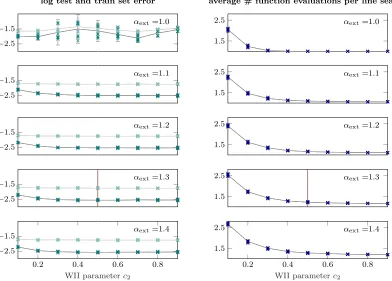
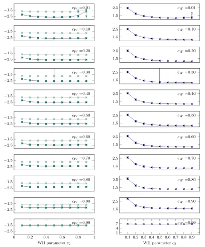
Figure 10: Sensitivity to varying hyper-parameters c2, and cW. Plot and color coding as
in Figure 9 but this time for varyingcW instead of αext. Right Column: Again a low number indicates an efficient line search procedure (perfect efficiency at 1). For most parameter combinations this lies around ≈ 1.3−1.5. Only at extreme parameter values for examplecW = 0.99, which amounts to imposing
per line search, both versus different choices of Wolfe parameterc2. The left column thus shows the overall performance of the optimizer, while the right column is representative for the computational efficiency of the line search. Intuitively, a line search which is minimally invasive (only corrects the learning rate, when it is really necessary) is preferred. Rows in Figure 10 show the same plot for different choices of the Wolfe thresholdcW.
The effect of strict c2 can be observed clearly in Figure 10 where for smaller values of c2 <≈ 0.2 the average number of function evaluations spend in one line search goes up slightly in comparison to looser restrictions onc2, while still a very good perfomace is reached in terms of train and test set error. Likewise, the last row of Figure 10 for the extreme value ofcW = 0.99 (demanding 99% certainty about the validity if the Wolfe conditions),
shows significant loss in computational efficiency having an average number of 7 function evaluations per line search. Besides loosing efficiency, it is still optimizing the objective well. Lowering this threshold a bit to 90% increases the computational efficiency of the line search to be nearly optimal again.
Ideally, we want to trade off the desiderata of being strict enough to reject too small and too large steps that prevent the optimizer to converge, but being lenient enough to allow all other reasonable steps, thus increasing computational efficiency. The valuescW = 0.3 and
c2 = 0.5, which are adopted in our current implementation are marked as dark red vertical lines in Figure 10.
4.2.2 Extrapolation Factor αext
The extrapolation parameter αext, introduced in Section 3.4.4, pushes the line search to try a larger learning rate first, than the one which was accepted in the previous step. Figure 9 is structured like Figure 10, but this time explores the line search sensitivity in thec2-αext parameter space (abscissa and rows respectively) while keepingcW fixed at 0.3. Unless we
chooseαext= 1.0 (no step size increase between steps) in combination with a lenient choice of c2 the line search performs well. For now we adopt αext = 1.3 as default value which again is shown as dark red vertical line in Figure 9.
The introduction ofαextmight seem arbitrary at first, but is a necessity and well-working fix because of a few shortcomings of the current design. First, the curvature condition W-II is the single condition that prevents too small steps and pushes optimization progress. On the other hand both W-I and W-II simultaneously penalize too large steps (see Figure 1 for a sketch). This is not a problem in case of deterministic observation (σf, σf0 →0), where W-II undoubtedly decides if a gradient is still too negative. Unless W-II is chosen very tightly (small c2) or cW unnecessarily large (both choices, as discussed above, are undesirable),
in the presence of noise, pWolfe will thus be more reliable in preventing overshooting than pushing progress. The first row of Figure 9 illustrates this behavior, where the performance drops somewhat if no extrapolation is done (αext = 1.0) in combination with a looser version of W-II (largerc2).
inevitable bias is introduced of approximate size of cos−1(γ) (where γ is the expected angle between gradient evaluations from two independent mini-batches at t= 0). Since the scale parameterθ of the Wiener process is implicitly set byy0(0) (§3.4.2), thegpbecomes more uncertain at unobserved points than it needs to be; or alternatively expects the 1D-gradient to cross zero at smaller steps, and thus underestimates a potential learning rate. The posteriorat observed positions is little affected. The over-estimation ofθrather pushes the posterior towards the likelihood (since there is less model to trust) and thus still gives a reliable measure forf(t) andf0(t). The effect on the Wolfe conditions is similar. With y0(0) biased towards larger values, the Wolfe conditions, which measure the drop in projected gradient norm, are thus prone to accept larger gradients combined with smaller function values, which again is met by making small steps. Ultimately though, since candidate points attcand >0 that are currently queried for acceptance, are always observed and unbiased, this can be controlled by an appropriate design of the Wolfe factorc2 (§3.4.1 and §4.2.1) and of course αext.
4.2.3 Full Hyper-Parameter Search: cW-c2-αext
An exhaustive performance evaluation on the wholecW-c2-αext-grid is shown in Appendix C in Figures 20-24 and Figures 25-35. As discussed above, it shows the necessity of introducing the extrapolation parameter αext and shows slightly less efficient performance for obviously undesirable parameter combinations. In a large volume of the parameter space, and most importantly in the vicinity of the chosen design parameters, the line search performance is stable and comparable to carefully hand tuned learning rates.
4.2.4 Safeguarding Mis-scaled gps: θreset
For completeness, we performed an additional experiment on the threshold parameter which is denoted byθreset in the pseudo-code (Appendix D) and safeguards against gp mis-scaling. The introduction of noisy observations necessitates to model the variability of the 1D-function, which is described by the kernel scale parameterθ. Setting this hyper-parameter is implicitly done by scaling the observation input, assuming a similar scale than in the previous line search (§3.4.2). If, for some reason, the previous line search accepted an unexpectedly large or small step (what this means is encoded inθreset) thegpscaleθfor the next line search is reset to an exponential running average of previous scales (αstats in the pseudo-code). This occurs very rarely (for the default value θreset = 100 the reset occurred in 0.02% of all line searches), but is necessary to safeguard against extremely mis-scaled gp’s. θreset therefore is not part of the probabilistic line search model as such, but prevents mis-scaled gps due to some unlucky observation or sudden extreme change in the learning rate. Figure 8 shows performance of the line search for θreset = 10,100,1000 and 10 000 showing no significant performance change. We adoptedθreset= 100 in our implementation since this is the expected and desired multiplicative (inverse) factor to maximally vary the learning rate in one single step.
4.3 Candidate Selection and Learning Rate Traces
0.5 1.0 1.5 2.0 2.5 ·104 −3
−2 −1
# line searches
pWolfeonly −3
−2
−1 uEI·pWolfe
−3 −2 −1
log
learning
rate u
EIonly −3
−2 −1 0
# function evaluations
log
test
and
train
set
error
−3 −2 −1 0
m =100
−3 −2 −1 0
log
learning
rate m =200
0 0.5 1 1.5 2 2.5 3 3.5 4
·104 −2
0
# line searches
m =1000
Figure 12: Traces ofaccepted logarithmic learning rates. All runs are performed with default design parameters. Different rows show the same plot for different mini-batch sizes of m= 100,200 and 1000; plots and smoothing as in rows 2-4 of Figure 11 (details in text).
−1 0 1 2 3
log
σf
−3.5 −3 −2.5 −2
log
σdf
0 0.2 0.4 0.6 0.8 1 1.2 1.4 1.6 1.8 2 2
4 6
# line searches in 104
a
v
erage
#
of
f-ev
als
m=1000 m=200 m=100
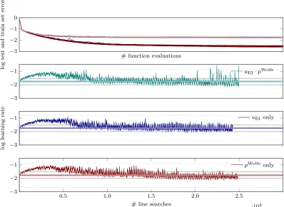
candidate point tcandi ; then choosing the one with the highest value for evaluation of the objective (§3.2). The Wolfe probability pWolfe actually encodes precisely what kind of point we want to find and incorporates both (W-I and W-II) conditions about the function valueand to the gradient (§3.3). However pWolfe does not have very desirable exploration properties. Since the uncertainty of thegpgrows to ‘the right’ of the last observation, the Wolfe probability quickly drops to a low, approximately constant value there (Figure 4). Also pWolfe is partially allowing for undesirably short steps (§4.2.2). The expected improvement uEI, on the other hand, is a well studied acquisition function of Bayesian optimization trading off exploration and exploitation. It aims to globally find a point with a function value lower than a current best guess. Though this is a desirable property also for the probabilistic line search, it is lacking the information that we are seeking a point that also fulfills the W-II curvature condition. This is evident in Figure 4 where pWolfe significantly drops at points where the objective function is already evaluated but uEI does not. In addition, we do not need to explore the positivetspace to an extend, the expected improvement suggests, since the aim of a line search is just to find a good, acceptable point at positive t and not the globally best one. The product of both acquisition function uEI·pWolfe is thus a trade-off between exploring enough, but still preventing too much exploitation in obviously undesirable regions. In practice, though, we found that all three choices ((i) uEI·pWolfe, (ii) uEI only, (iii) pWolfe only) perform comparable. The following experiments were all
performed training N-II on MNIST; only the mini-batch size might vary as indicated. Figure 11 compares all three choices for mini-batch size m = 200 and default design parameters. The top plot shows the evolution of the logarithmic test and train set error (for plot and color description see Figure caption). All test and train set error curves respectively bundle up (only lastly plotted clearly visible). The choice of acquisition function thus does not change the performance here. Rows 2-4 of Figure 11 show learning rate traces of a single seed. All three curves show very similar global behavior. First the learning rate grows, then drops again, and finally settles around the best found constant learning rate. This is intriguing since on average a larger learning rate seems to be better at the beginning of the optimization process, then later dropping again to a smaller one. This might also explain why sgd+probLSin the first part of the optimization progress outperforms vanilla sgd (Figure 7). Runs that use just slightly larger constant learning rates than the best performing constant one (above the gray horizontal lines in Figure 11) were failing after a few steps. This shows that there is some non-trivial adaptation going on, not just globally, but locally at every step.
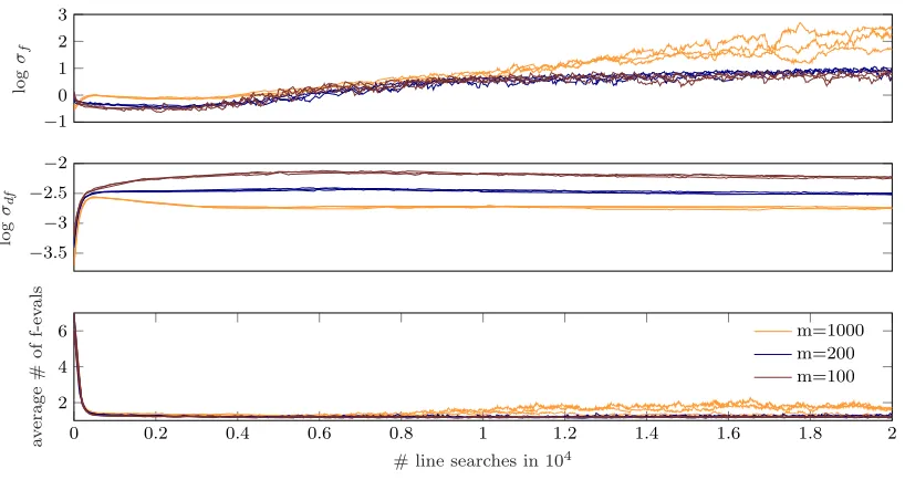
Figure 12 shows traces of accepted learning rates for different mini-batch sizes m = 100,200,1000. Again the global behavior is qualitatively similar for all three mini-batch sizes on the given architecture. For the largest mini-batch size m= 1000 (last row of Figure 12) the probabilistic line search accepts a larger learning rate (on average and in absolute value) than for the smaller mini-batch sizesm= 100 and 200, which is in agreement with practical experience and theoretical findings (Hinton (2012,§4 and 7), Goodfellow et al. (2016,§9.1.3), Balles et al. (2016)).
process, in comparison to≈1.5 for m= 100,200. This seems counter intuitive in a way, but since larger mini-batch sizes also observe smaller value and gradients (especially towards the end of the optimization process), the relative noise levels might actually be larger. (Although the curves for varying m are shown versus the same abscissa, the corresponding optimizers might be in different regions of the loss surface, especially m = 1000 probably reaches regions of smaller absolute gradients). At the start of the optimization the average number of function evaluations is high, because the initial default learning rate is small (10−4) and the line search extends each step multiple times.
5. Conclusion
The line search paradigm widely accepted in deterministic optimization can be extended to noisy settings. Our design combines existing principles from the noise-free case with ideas from Bayesian optimization, adapted for efficiency. We arrived at a lightweight “black-box” algorithm that exposes no parameters to the user. Empirical evaluations so far show compatibility with the sgd search direction and viability for logistic regression and multi-layer perceptrons. The line search effectively frees users from worries about the choice of a learning rate: Any reasonable initial choice will be quickly adapted and lead to close to optimal performance. Our matlab implementation can be found athttp: //tinyurl.com/probLineSearch.
Acknowledgments
Appendix A. – Noise Estimation
Section 3.4.3 introduced the statistical variance estimators
Σ0(x) = (1−m)−1( ˆ∇S(x)− ∇Lˆ(x)2)
Σ(x) = (1−m)−1( ˆS(x)−Lˆ(x)2) (19) of the function and gradient estimate ˆL(x) and ∇Lˆ(x) at position x. The underlying assumption is that ˆL(x) and ∇Lˆ(x) are distributed according to
ˆ L(x)
∇Lˆ(x)
∼ N Lˆ(x) ∇Lˆ(x)
;
L(x)
∇L(x)
,
Σ(x) 0D×1 01×D diag Σ0(x)
(20)
which implies Eq 3
ˆ
L(x) s(x)0· ∇Lˆ(x)
=
y(x) y0(x)
∼ N f(x)
f0(x)
,
σf(x) 0
0 σf0(x)
. (21)
wheres(x) is the possibly new search direction atx. This is an approximation since the true covariance matrix is in general not diagonal. A better estimator for the projected gradient noise would be (droppingx from the notation)
ηf0 =s|
"
1 m−1
1 m
m X
k=1
(∇`k− ∇Lˆ)(∇`k− ∇Lˆ)|
# s = D X i,j=1
sisj
1 m−1
1 m m X k=1
∇`ki − ∇Lˆi ∇`kj − ∇Lˆj
= 1
m−1
D X
i,j=1
sisj
1 m
m X
k=1
∇`ki∇`kj − ∇Lˆi∇Lˆj− ∇Lˆj∇Lˆi+∇Lˆi∇Lˆj !
= 1
m−1
1 m m X k=1 D X i,j=1
si∇`kisj∇`kj − D X
i,j=1
sj∇Lˆjsi∇Lˆi
= 1
m−1 1 m
m X
k=1
(s0· ∇`k)2−(s0· ∇Lˆ)2
!
.
(22)
Comparing to σf0 yields
ηf0 = 1 m−1
D X
i,j=1
sisj
1 m
m X
k=1
∇`ki∇`kj − ∇Lˆj∇Lˆi !
= 1
m−1
D X
i=1
s2i 1 m
m X
k=1
(∇`ki)2− ∇Lˆ2i !
+ 1
m−1
D X i6=j=1
sisj
1 m
m X
k=1
∇`ki∇`kj − ∇Lˆj∇Lˆi !
ηf0 =σf0 + 1 m−1
D X i6=j=1
sisj
1 m
m X
k=1
∇`ki∇`kj − ∇Lˆj∇Lˆi !
.
From Eq 22 we see that, in order to effectively compute ηf0, we need an efficient way of computing the inner product (s0· ∇`k) for allk. In addition, we need to know the search direction s(x) of the potential next step (if x was accepted) at the time of computing ηf0. This is possible e.g. for the sgdsearch direction where s(x) =−m1 Pmk=1∇`k(x) but potentially not possible or practical for arbitrary search directions. For all experiments in this paper we used the approximate variance estimatorσf0.
The following paragraph is concerned with the independence assumption of gradient and function valuey andy0 (in contrast to independence among gradient elements). In generaly and y0 are not independent since the algorithm draws them from the same mini-batch; the likelihood including the correlation factorρ reads
p(yt, yt0|f) =N
yt
y0t
;
f(t) f0(t)
,
σ2f ρ ρ σf20
. (24)
The noise covariance matrix enters the gp only in the inverse of the sum with the kernel matrix of the observations. We can compute it analytically for one datapoint at position t, since it is only a 2×2 matrix. Forρ= 0, define:
detρ=0:= [ktt+σf2][∂ ∂k tt+σf20]−k∂tt∂ktt
G−ρ=01 :=
ktt+σf2 k∂tt
k
∂
tt ∂ ∂k tt+σf20
−1
= 1
detρ=0
k
∂ ∂
tt+σf20 −k∂tt
−∂ktt ktt+σf2
. (25)
Forρ6= 0 we thus get:
detρ6=0:= [ktt+σ2f][∂ ∂k tt+σ2f0]−[k∂tt+ρ][∂ktt+ρ]
=detρ=0−ρ(∂ktt+k∂tt)−ρ2
G−ρ6=01 :=
ktt+σf2 k∂tt+ρ
k
∂
tt+ρ ∂ ∂k tt+σf20
−1
= 1
detρ6=0
k
∂ ∂
tt+σf20 −(k∂tt+ρ)
−(∂ktt+ρ) ktt+σf2
= detρ=0 detρ6=0
G−ρ=01 − ρ
detρ6=0
0 1 1 0
(26)
The fraction detρ=0/detρ6=0 in the first term of the last row, is a positive scalar that scales all element of G−ρ=01 equally (since Gρ=0 andGρ6=0 are positive definite matrices, we know that detρ=0 >0,detρ6=0>0). If |ρ|is small in comparison to the determinant detρ=0, then detρ6=0 ≈ detρ=0 and the scaling factor is approximately one. The second term corrects off-diagonal elements inGρ6=0 and is proportional to ρ; if |ρ| detρ=0 this term is small as well.
Appendix B. – Noise Sensitivity
−4 −2 0
m:1000
−4 −2 0
m:100
−4 −2 0 −3
−2 −1 0
log learning rate
log
test
and
train
set
error
m:10
−4 −2 0
m:200
0 1 2 3 4 0 1 2 3 4
0 1 2 3 4
0 1 2 3 4
−3 −2 −1 0
log
train
set
er
ror
0 1 2 3 4 0 1 2 3 4
0 1 2 3 4
0 1 2 3 4
−1 0
# function evaluations in 104
log
test
set
erro
r
−4 −2
m:1000
−4 −2 0
0.3 0.6 0.9
log learning rate
test
and
train
se
t
error
m:10
−4 −2
m:100
−4 −2
m:200
0 0.5 1
0 0.5 1
0 0.5 1
0 0.5 1
0 0.3 0.6 0.9
train
set
error
0 0.5 1
0 0.5 1
0.6 0.7 0.8 0.9
# function evaluations in 104
test
set
error
0 0.5 1 0 0.5 1