Explaining the Success of AdaBoost and Random Forests as
Interpolating Classifiers
Abraham J. Wyner [email protected]
Matthew Olson [email protected]
Justin Bleich [email protected]
Department of Statistics
Wharton School, University of Pennsylvania Philadelphia, PA 19104, USA
David Mease [email protected]
Apple Inc.
Editor:Koby Crammer
Abstract
There is a large literature explaining why AdaBoost is a successful classifier. The literature on AdaBoost focuses on classifier margins and boosting’s interpretation as the optimiza-tion of an exponential likelihood funcoptimiza-tion. These existing explanaoptimiza-tions, however, have been pointed out to be incomplete. A random forest is another popular ensemble method for which there is substantially less explanation in the literature. We introduce a novel per-spective on AdaBoost and random forests that proposes that the two algorithms work for similar reasons. While both classifiers achieve similar predictive accuracy, random forests cannot be conceived as a direct optimization procedure. Rather, random forests is a self-averaging, interpolating algorithm which creates what we denote as a “spiked-smooth” classifier, and we view AdaBoost in the same light. We conjecture that both AdaBoost and random forests succeed because of this mechanism. We provide a number of examples to support this explanation. In the process, we question the conventional wisdom that sug-gests that boosting algorithms for classification require regularization or early stopping and should be limited to low complexity classes of learners, such as decision stumps. We con-clude that boosting should be used like random forests: with large decision trees, without regularization or early stopping.
Keywords: AdaBoost, random forests, tree-ensembles, overfitting, classification
1. Introduction
In the “boosting” approach to machine learning, a powerful ensemble of classifiers is formed by successively refitting a weak classifier to different weighted realizations of a data set. This intuitive procedure has seen a tremendous amount of success. In fact, shortly, after its introduction, in a 1996 NIPS conference, Leo Brieman crowned AdaBoost (Freund and Schapire, 1996) (the first boosting algorithm) the “best off-the-shelf classifier in the world (Friedman et al., 2000).” AdaBoost’s early success was immediately followed by efforts to explain and recast it in more conventional statistical terms. The statistical view of boosting holds that AdaBoost is a stage-wise optimization of an exponential loss function
c
(Friedman et al., 2000). This realization was especially fruitful leading to new “boosting machines” (Friedman, 2001; Ridgeway, 2006) that could perform probability estimation and regression as well as adapt to different loss functions. The statistical view, however, is not the only explanation for the success of AdaBoost. The computer science literature has found generalization error guarantees using VC bounds from PAC learning theory and margins (Guestrin, 2006). While some research has cast doubt on the ability of any one of these to fully account for the performance of AdaBoost they are generally understood to be satisfactory (Schapire, 2013).
This paper parts with traditional perspectives on AdaBoost by concentrating our anal-ysis on the implications of the algorithm’s ability to perfectly fit the training data in a wide variety of situations. Indeed, common lore in statistical learning suggests that perfectly fitting the training data must inevitably lead to “overfitting.” This aversion is built into the DNA of a statistician who has been trained to believe, axiomatically, that data can always be decomposed into signal and noise. Traditionally, the “signal” is always modeled smoothly. The resulting residuals represent the “noise” or the random component in the data. The statistician’s art is to walk the balance between the signal and the noise, ex-tracting as much signal as possible without extending the fit to the noise. In this light, it is counterintuitive that any classifier can ever be successful if every training example is “interpolated” by the algorithm and thus fit without error.
The computer scientist, on the other hand, does not automatically decompose problems into signal and noise. In many classical problems, like image detection, there is no noise in the classical sense. Instead there are only complex signals. There are still residuals, but they do not represent irreducible random errors. If the task is to classify images into those with cats and without, the problem is hard not because it is noisy. There are no cats wearing dog disguises. Consequently, the computer scientist has no dogmatic aversion to interpolating training data. This was the breakthrough.
It is now well-known that interpolating classifiers can work, and work well. The Ad-aBoost classifier created a huge splash by being better than its established competitors (for instance, CART, neural networks, logistic regression) (Breiman, 1998) and substantively better than the technique of creating an ensemble using the bootstrap (Breiman, 1996). The statistics community was especially confounded by two properties of AdaBoost: 1) interpolation (perfect prediction in sample) was achieved after relatively few iterations, 2) generalization error continues to drop even after interpolation is achieved and maintained. The main point of this paper is to demonstrate that AdaBoost and similar algorithms work not in spite, but because of interpolation. To bolster this claim, we will draw a constant analogy with random forests (Breiman, 2001), another interpolating classifier. The random forests algorithm, which is also an ensemble-of-trees method, is generally regarded to be
among the very best commonly used classifiers (Manuel Fern´andez-Delgado and Amorim,
al-gorithmic property of fitting the training data completely without error. Each of these interpolating classifiers also exhibits a self-averaging property. We attempt to show that these two properties together make for a classifier with low generalization error. While it is easy to see that random forests has both of these mechanisms by design, it is less clear that this is true for AdaBoost.
It is worth noting that Breiman noticed the connection between random forests and AdaBoost as well, although his notion of a random forest was more general, including
other types of large ensembles of randomly grown trees (Breiman, 2001). In his 2001
Random Forests paper, he conjectured that the weights of AdaBoost might behave like
an ergodic dynamic system, converging to an invariant distribution. When run for a long time, the additional rounds of AdaBoost were equivalent to drawing trees randomly grown according to this distribution, much like a random forest. Recent work has followed up on this idea, proving that the weights assigned by AdaBoost do indeed converge to a invariant
distribution1(Belanich and Ortiz, 2012). In this work, the authors also show that functions
of these weights, such as the generalization error and margins, also converge. This work certainly complements ours, but we focus on the similarity between AdaBoost and random forests through the lens of the type of decision surfaces both classifiers produce, and ability of both algorithms to achieve zero error on the training set.
One of our key contributions will be to present a decomposition of AdaBoost as the weighted sum of interpolating classifiers. Another contribution will be to demonstrate the mechanism by which interpolation combined with averaging creates an effective classifier. It turns out that interpolation provides a kind of robustness to noise: if a classifier fits the data extremely locally, a “noise” point in one region will not affect the fit of the classifier at a nearby location. When coupled with averaging, the result is that the fit stabilizes at regions of the data where there is signal, while the influence of noise points on the fit becomes even more localized. It will be easy to see this point holds true for random forests. For AdaBoost, it is less clear, however, and a decomposition of AdaBoost and simulation results in Section 4 will demonstrate this crucial point. We will observe that the error of AdaBoost at test points near noise points will continue to decrease as AdaBoost is run for more iterations, demonstrating the localizing effect of averaging interpolating classifiers.
We will begin in Section 2 by critiquing some of the existing explanations of AdaBoost. In particular, we will discuss at length some of the shortcomings of the statistical optimiza-tion view of AdaBoost. In Secoptimiza-tion 3, we will discuss the merits of classificaoptimiza-tion procedures that interpolate the training data, that is, that fit the training data set with no error. The main conclusion from this section is that interpolation, done correctly, can provide robustness to a fit in the presence of noise. This discussion will be augmented with simu-lations discussing the performance of random forests, AdaBoost, and other algorithms in a noisy environment. We will then derive our central observation in Section 4, namely that AdaBoost can be decomposed as a sum of classifiers, each of which fits the training data perfectly. The implication from this observation is that for the best performance, we should run AdaBoost for many iterations with deep trees. The deep trees will allow the component classifiers to interpolate the data, while a large number of iterations will lend to a bagging
effect. We will then demonstrate this intuition in a real data example in Section 5. Finally, we conclude with a brief discussion in Section 6.
2. Competing Explanations for the Effectiveness of Boosting
In this section we will present an overview of some of the most popular explanations for the success of boosting, with analysis of both the strengths and weaknesses of each approach. Our emphasis will focus on the margins view of boosting and the statistical view of boosting, each of which has a large literature and has led to the development of variants of boosting algorithms. For a more extensive review of the boosting literature, one is well-advised to consult Schapire and Freund (2012).
Before we begin, we will briefly review the AdaBoost algorithm not only to refresh the reader’s mind, but also to establish the exact learning algorithm this paper will consider,
as there are many variants of AdaBoost. To this end, the reader is invited to review
Algorithm 1. In our setting, we are given N training points (xi, yi) where xi ∈ X and
yi ∈ {−1,+1}. On round m, where m = 1, . . . , M, we fit a weak classifier Gm(x) to a
version of the data set reweighted by some weighting vector wm. We then calculate the
weighted misclassification rate of our chosen learner, and update the weighting measure
used in the next round, wm+1. The final classifier is output as the sign of a weighted
linear combination of classifiers produced from each stage of the algorithm. In practice, one sometimes limits the number of rounds of boosting as a form of regularization. We will discuss this point more in the next section, and challenge its usefulness in later parts of the paper.
Algorithm 1:AdaBoost Hastie et al. (2009)
1. Initialize the observation weightswi=
1
N, i= 1,2, . . . , N.
2. Form= 1 to M:
(a) Fit a classifier Gm(x) to the training data using weights wi.
(b) Compute errm=
PN
i=1wiI(yi 6=Gt(xi))
PN
i=1wi
.
(c) Compute am= log
1−errt
errt
.
(d) Set wi←wi·exp (at·I(yi 6=Gt(xi)))
(e) Set fi(x) =PMm=1amGm(x)
3. Outputf(x) = sign (fM(x))
2.1 Margin View of Boosting
more rounds, it is able to fit the data increasingly well which should lead to overfitting. However, in practice we observe that running boosting for many rounds does not overfit in most cases. One of the first attempts to resolve this paradox was explored by Schapire
et al. (1998), who focused on the margins of AdaBoost. The margins can be thought of
as a measure of how confident a classifier is about how it labels each point, and one would hypothetically desire to produce a classifier with margins as large as possible. Schapire et al. (1998) proved that AdaBoost’s generalization error decreases as the size of the margins increase. Indeed, in practice one observes that as AdaBoost is run for many iterations, test error decreases while the size of the empirical margins increase. In fact, recent research has demonstrated that AdaBoost can be reformulated exactly as mirror descent applied to the problem of maximizing the smallest margin in the training set under suitable separability conditions (Freund et al., 2013).
One could take these observations to suggest that a more effective algorithm might be designed to explicitly optimize margins. However, one can find evidence against this
hypothesis in Breiman’s arc-gv algorithm (Breiman, 1999). Breiman designed the arc-gv
algorithm to maximize the minimum margin in a data set, and he found that this algorithm actually had worse generalization error than AdaBoost. Moreover, he developed generaliza-tion error bounds based on the minimum margin of a classifier which were tighter than those established by Shapire, casting doubt on the existing margin explanation. Other algorithms
designed to maximize margins, such as LP-Boost have also been found to perform worse
than AdaBoost in practice (Wang et al., 2011). Critics of these supposed counterexamples to the margin view of boosting note that AdaBoost’s success likely depends on the entire distribution of margins on the data, not just the smallest margin. More recent work has improved upon the Breiman’s generalization bound by taking into account other aspects of the margin that more closely reflect its distribution, adding new life to the margin ex-planation of AdaBoost (Gao and Zhou, 2013). While the margin exex-planation of AdaBoost is certainly intuitive, its role in producing low generalization error is still an area of active research.
2.2 Statistical Optimization View of Boosting
Friedman et al. (2000) take great strides to clear up the mystery of boosting to provide statisticians with a statistical view of the subject. The heart of their article is the recasting of boosting as a statistically familiar program for finding an additive model by means of a forward stage-wise approximate optimization of an exponential criterion. In short, this view places boosting firmly in classical statistical territory by clearly defining it as a procedure
to search through the space of convex combinations ofweak learners orbaseclassifiers. This
Although the statistical optimization perspective of AdaBoost is surely interesting and informative, there remain problems. First, we observe that the fact that AdaBoost mini-mizes an exponential loss may not alone account for its performance as a classifier. Wyner (2003) introduces a variant of AdaBoost called Beta-Boost which is very similar to AdaBoost except that by design the exponential loss function is constant throughout the iterations. Despite this, Beta-Boost was able to demonstrate similar performance to AdaBoost on simulated data sets. Furthermore, among many similar examples in the literature, Mease and Wyner (2008) present a simulation example in which the the exponential loss is mono-tonically increasing with the number of iterations of AdaBoost on a test set, while the generalization error decreases. In this example, the value of the exponential loss is uninfor-mative about how well the classifier generalizes. Freund et al. (2013) also provide evidence to this end. They conduct an experiment that compares AdaBoost to two AdaBoost variants that minimize the exponential loss function at differing rates: one performs the minimiza-tion very quickly through gradient descent, while the other performs the minimizaminimiza-tion quite slowly. They find that AdaBoost performed significantly better than these two competitors, suggesting that AdaBoost’s strong performance cannot be tied exclusively to its action on the exponential loss function.
We also contend that some of the mathematical theory connected with the statistical optimization view of boosting has a disconnect with the types of boosting algorithms that work in practice. The optimization theory of boosting insists that overfitting can be avoided
by requiring the set of weak learners, to be just that: weak. B¨uhlmann and Yu (2003)
argues that one can avoid overfitting by employing regularization with weak base learners. However, empirical evidence points to quite the opposite: boosting deep trees for many iterations tends to produce a better classifier than boosted stumps with regularization (Mease and Wyner, 2008). The use of early-stopping as a form of regularization has also been called into question (Mease and Wyner, 2008). The thrust of our paper will be to
demonstrate why weshould actually expect boosting with deep trees run for many iterations
to have better generalization error. Recent work also suggests that boosting low complexity classifiers may not be able to achieve good accuracy in difficult classification tasks such as speech recognition or image recognition (Cortes et al., 2014). This paper proposes an algorithm called “DeepBoost” which encourages boosting high complexity base classifiers— such as very deep decision trees—but in a “capacity-conscious” way. One last problem with theory associated with the statistical view of boosting is that by its very nature it suggests that we should be able to extract conditional class probability estimates from the boosted fit, as the procedure is apparently maximizing a likelihood function. Mease and Wyner (2008), however, point out a number of examples where the implied conditional class estimates from the boosting fit diverge to zero and one. While boosting appears to do an excellent job as a classifier, it apparently fails to estimate probability quantiles correctly.
We can now summarize the main empirical contradictions with existing theoretical ex-planations of boosting, which motivates the view we present in this paper:
1. Boosting works well, perhaps best in terms of performance if not efficiency, with “strong learners” like C4.5 and CART (Niculescu-Mizil and Caruana, 2005).
3. The optimization theory offers no explanation as to why the training error can be zero, yet the test error continues to descend (Freund and Shapire, 2000)
This paper will squarely depart from the statistical optimization view by asserting that AdaBoost may be best thought of as a (self) smoothed, interpolating classifier. We will see that unlike the statistical optimization view, this perspective suggests that for best performance once should run many iterations of AdaBoost with deep trees. This will allow us to draw a number of analogies between AdaBoost and random forests. A key component to this argument will consist of explaining the success of interpolating classifiers in noisy environments. We will pursue this line of thought in the following section.
3. Interpolating Classifiers
Algorithm 2:Random Forests Hastie et al. (2009)
1. Forb= 1 to B:
(a) Draw a bootstrap sample X∗ of sizeN from the training data
(b) Grow a decision tree Tb to the dataX∗ by doing the following recursively
until the minimum node size nmin is reached:
i. Select m of thep variables
ii. Pick the best variable/split-point from the m variables and partition
2. Output the ensemble{Tb}Bb
Let ˆCb(x∗) be predicted class of tree Tb. Then ˆCrfB(x
∗) = majority vote{Cˆ
b(x∗)}B1.
It is a widely held belief by statisticians that if a classifier interpolates all the data, that is, it fits all the training data without error, then it cannot be consistent and should have a poor generalization error rate. In this section, we demonstrate that there are interpolating classifiers that defy this intuition: in particular, AdaBoost and random forests will serve as leading examples of such classifiers. We argue that these classifiers achieve good out of sample performance by maintaining a careful balance between the complexity required to perfectly match the training data and a general semi-smoothness property. We begin with a quick review of the random forests classifier, which will be in constant analogy with AdaBoost.
3.1 Random Forests
Random forests has gained tremendous popularity due to robust performance across a wide range of data sets. The algorithm is often capable of achieving best-in-class performance with respect to low generalization error and is not highly sensitive to choice of tuning parameters, making it the off-the-shelf tool of choice for many applications.
Algorithm 2 reviews the procedure for constructing a random forests model. Note that in
many popular implementations, such asRimplementation randomForestLiaw and Wiener
(2002) built from Breiman’s CART software, nmin is set to one for classification. This
necessarily interpolates the data in its bootstrap sample (assuming as least one continuous predictor). This results in each tree being a low bias but high variance estimator. Variance is then reduced by averaging across trees, resulting in a “smoothing” of the estimated response surface. The random predictor selection within each tree further reduces variance by lowering the correlation across the trees. The final random forest classifier still fits the entire training data set perfectly, at least with very high probability. To see this is true, consider any given training point. As the number of trees increases, with probability close to one, that point will be present in the majority of the bootstrap samples used to fit the trees in the forest. Thus the point will get the correct training set label when the votes are tabulated to determine the final class label.
We wish to emphasize that despite its success, random forests is not directly optimizing any loss function across the entire ensemble; each tree is grown independently of the other trees. While each tree may optimize a criteria such as the Gini index, the full ensemble is not constructed in any optimization-driven fashion such as is the case for AdaBoost. While there has been recent theoretical work describing the predictive surface of random forests (Wager and Walther, 2015), the analysis required unnatural assumptions that are hard to justify in practice (such as the growth rate of minimum leaf size). Rather, we postulate that the success of the algorithm is due to its interpolating nature plus the self-averaging mechanism. We next consider the implications of interpolating classifiers more broadly.
3.2 Local Robustness of Interpolating Classifiers
Let us begin with a definition of interpolation:
Definition: LetXi be vector observations of predictor variables a letYi be the observed
class label. A classifierf(X) is said to be aninterpolatingclassifier if for every training set
example, the classifier assigns the correct class label; that is for every i,f(Xi) =Yi.
The term “interpolation” is likely jarring for some readers. In many contexts, one
often thinks about interpolating a set of points with classically smooth functions, such as polynomial splines. However, strictly speaking, there are many other ways that one might interpolate a set of points—through the fit of an AdaBoost classifier, for instance! Since the notion of fitting a set of points without error is central to this paper, and since the common definition of interpolation does not preclude the kinds of fits we consider, we felt it appropriate to proceed with the term.
One of our key insights reverses the common intuition about classifiers: interpolation can prevent overfitting. An interpolated classifier, if sufficiently local, minimizes the influence of noise points in other parts of the data. In order to make this point conceptually clear, it is helpful to put ourselves in familiar territory with a regression example.
Suppose we are trying to predict a continuous response ybased on real-valuedx
obser-vations. Let us assume that the true underlying model is y =x+, where is a mixture
of a point mass at zero and some heavy-tailed distribution. In other words, we’ll assume
that most points in a given training set reflect the true linear relationship between y and
x, but a few observations will be noise points. This is analogous to the types of probability
models we typically consider in classification settings, such as those found in later sections of the paper. Figure 1 shows hypothetical training data: note that the only “noise” point
is found at x= 0.4. We then consider fitting three models to this data: two interpolating
functions, given by the blue and black lines, and an ordinary regression fit given by the red line. The first thing to notice is that the two interpolating fits differ only from the
true target mean model y = x only at the noise point x = 0.4. In contrast, the fit of the
regression line deviates from the underlying target over the entire range ofx. The one noise
point corrupted the entire fit of the regression line, while the interpolating lines were able to minimize the influence of the noise point by adapting to it only very locally. Moreover, one should note that between the two interpolating fits, the blue line interpolates more locally than the black line, and thus its overall fit is even less influenced by the noise point. This simplified example is of course meant to be didactic, but we will show throughout the rest of this paper that in practice AdaBoost and random forest do indeed produce fits similar to the blue line.
0.0 0.2 0.4 0.6 0.8 1.0
0.0
0.2
0.4
0.6
0.8
1.0
x
y
While it is conceptually clear that it is desirable to produce fits like the blue interpolating line in the previous example, one may wonder how such fits can be achieved in practice. In the classification setting, we will argue throughout this paper that this type of fit can be realized through the process of averaging interpolating classifiers. We will refer to the
decision surface produced by this process as being spiked-smooth. The decision surface is
spiked in the sense that it is allowed to adapt in very small regions to noise points, and it
issmooth in the sense that it has been produced through averaging. A technical definition
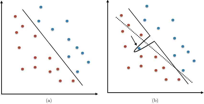
of a spiked-smooth decision surface would lead us too far astray. It may be helpful instead to consider the types of classifiers that do not produce a spiked-smooth decision surface, such as a logistic regression. Logistic regression separates the input space into two regions with a hyperplane, making a constant prediction on each region. This surface is not spiked-smooth because it does not allow for local variations: in large regions (namely, half-spaces), the classifier’s predictions are constrained to be the same sign. Figure 2 provides a graphical illustration of this intuition.
(a) (b)
Figure 2: An illustration of the robustness to noise of interpolating classifiers. In 2a a classifier (such as a logistic regression) is fit to a set of training data, and the decision boundary produced by this classifier is shown as a solid line. In 2b, the same type of classifier is fit to the training data, except a noise point is added to the data (the blue point marked by the arrow). The one noise point shifts the entire decision boundary, which is shown as the dotted line. On the other hand, the decision boundary produced by a classifier which interpolates very locally is shown as a solid line. It is clear that this classifier is able to adapt locally to the noise point, and the overall fit does not get corrupted.
the same way. Classically smooth classifiers—such as logistic regression or pruned CART trees—are forced to produce fits that are locally constant. It is harder for such classifiers to “recover” from making a mistake at a noise point since the surface of the fit will affect the fit at nearby points. Interpolating classifiers are flexible enough to make mistakes in “small regions.” When averaged over many such classifiers, the influence of the noise point can be easily smoothed out. Later examples in the paper will visualize this process, and will demonstrate that the later iterations of AdaBoost have a smoothing effect which shrinks down the influence of noise points on the overall fit of the classifier.
With this discussion in mind, let us consider another conceptual example, this time
in the classification setting. Suppose we have have two predictors x1 and x2 distributed
independently and uniformly on [0,1]2 and y ∈ {−1,+1}. Further suppose that the true
conditional class probability function is
P(x) =P(y= 1|x) =p=.75
for allx. This is a pure noise model with no signal, but in general one could view this as a
subspace of a more complex model in which the P(x) function is approximately constant.
Since the Bayes decision rule is to classify every point as a “+1”, we would desire an algorithm that will match the Bayes rule as close as possible. Again, we stress that this closeness should be judged with respect to the population or a hold-out sample. On this training data, any interpolating classifier will necessarily differ from the Bayes rule for
1−p= 25% of the points on average.
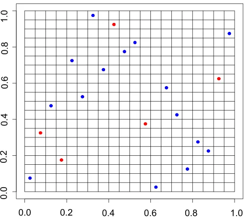
Figure 3 shows a possible sample of training data from this model of size n = 20.
The blue points represent the “+1”’s and the red points represent the “-1”’s. There are
5/20 = 25% red points. The training data was sampled according to a Latin Hypercube
design using the midpoints of the squares so that the points would be evenly spaced, but that is not essential.
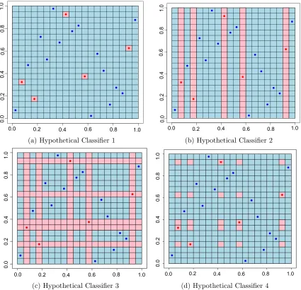
Figure 4 shows four hypothetical classifiers that could result from fitting boosted decision tree models to the training data in Figure 3. When decision trees are used as base learners for data with continuous predictors, it is a common convention to restrict the split points of the trees to be the midpoints of the predictors in the training data. Consequently, the classifier in each small square shown in Figure 3 will necessarily be constant throughout; this is the finest resolution of the classifier resulting from boosting decision tress assuming no sub-sampling. Thus, Figure 4a represents the interpolating classifier closest to the Bayes rule. (In these plots, pink squares represent “-1”’s and light blue squares represent “+1”’s.) Note that the interpolation is in fact quite local; the estimated function varies rapidly in the small neighborhoods of the pink squares. For such a classification rule the percentage of points in a hold-out sample that would differ from the Bayes rule (in expectation over
training sets) would be (1−p)n/nd where p =P(y= 1|x) and dis the dimensionality of
the predictor space (for our example, d= 2). We will present evidence later that in noisy
environments boosting sufficiently large trees does actually tend to find such rules as that in Figure 4a. Interestingly, since
lim
n→∞(1−p)n/n
d= 0
Figure 3: Training Data
vanishing measure, it is possible to obtain consistency in the limit as n→ ∞, even while
classifying every training point correctly. This stands in direct contrast to the conclusion of others such as Bickel et al. (2006) who have observed that the “empirical optimization problem necessarily led to rules which would classify every training set observation correctly
and hence not approach the Bayes rule whatever be n.”
While a classifier such as that in Figure 4a would preform well and is even consistent, many possible interpolators exist, such as the others displayed in Figure 4. Figure 4b shows
the (hypothetical) result of allowing the boosting algorithm to use trees involving only x1
and notx2. It is interesting to note that this classifier has severely overfit, even though it is
a simpler model, depending on only one of the two predictors. The classifier in Figure 4c has an even worse error rate, while the classifier in Figure 4d differs from the Bayes rule with
rate ((1−p)n)2/n2. This final example illustrates the type of structure and error rate that
occurs when stumps are used as the weak learner. In fact, Mease and Wyner (2008) show that the additive nature of stumps results in boosted classifiers that differ from the Bayes
rule at a rate of at least (1−p)d(1−1/d)dand hence is not consistent. The reason for this is
that using linear combinations of stumps does not provide enough flexibility to interpolate locally around points for which the observed class differs from the Bayes rule. In contrast, boosting larger trees, such as those grown in random forests interpolating with spikes of
increasingly smaller size. Some simulations demonstrating the superior performance of
larger trees over stumps are given in Mease and Wyner (2008) and here in Section 4.3.
1.0 0.8 0.6
0.4 0.2
0.0
0.0
0.2
0.4
0
.6
1
.0
0
.8
(a) Hypothetical Classifier 1
1.0 0.8
0.6 0.4
0.2 0.0
0.0
0.2
0
.4
0
.6
0
.8
1
.0
(b) Hypothetical Classifier 2
(c) Hypothetical Classifier 3 (d) Hypothetical Classifier 4
Figure 4: Four different hypothetical classifiers on a pure noise response surface where
many individually overfit classifiers, similar to the one in Figure 4b. The final result is a robust classifier, that is spiked-smooth; it fits the noise but only extremely locally.
3.3 A Two-Dimensional Example with Pure Noise
We will begin with an easy to visualize example that demonstrates how fine interpolation can provide robustness in a noisy setting. In particular, we compare the performance of AdaBoost, random forests and one-nearest neighbors, which are all interpolating classifiers. We will see see graphically that AdaBoost and random forests interpolate more locally around error points in the training data than the one-NN classifier. Consequently, AdaBoost and random forests are less affected by noise points as one-NN and have lower generalization error. We will show that the self-averaging property of AdaBoost and random forests is crucial. This property will be discussed in subsequent sections.
The implementation of AdaBoost is carried out according to the algorithm described
earlier. The base learners used are trees fit by therpartpackage (Therneau and Atkinson,
1997) inR. The trees are grown to a maximum depth of 8, meaning they may have at most
28 = 256 terminal nodes. This will be the implementation of AdaBoost we will consider
throughout the remainder of this paper.
We will consider again the “pure noise” model as described in the previous section,
where the probability that y is equal to +1 for every xis some constant value p > .5. For
the training data we will take n= 400 points uniformly sampled on [0,1]2 according to a
Latin Hypercube using the midpoints as before. For the correspondingy values in training
data we will randomly choose 80 points to be −1’s so that P(y= 1|x) =.8.
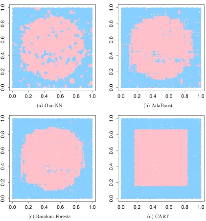
Figure 5 displays the results for the following: (a) one-NN, (b) AdaBoost , and (c) random forests. Regions classified as +1 are colored light blue and regions classified as
−1 are colored pink. The training data is displayed with blue points for y = +1 and
red points for y = −1. Since the Bayes’ rule would be to classify every point as +1, we
judge the performance of the classifiers by the fraction of the unit square that matches the Bayes’ rule. The nearest neighbor rule in this example classifies 79% of the region as +1
(we expect p = 80% on average for the one-NN) while AdaBoost performs substantially
better classifying 87% of the square as +1 after 100 iterations (which is long after the training error equals zero). This is evidence of boosting’s robustness to noise discussed in the previous section. The random forests (with 500 trees) does even better, classifying 94% of the figure as +1. Visually, it is obvious that the random forests and AdaBoost classifier is more spiked-smooth than one-nearest neighbors, which allows it to be less sensitive to noise points. AdaBoost and random forests do in fact overfit the noise—but only the noise. They do not allow the overfit to metastasize to modestly larger neighborhoods around the errors. It is interesting to note that there seems to be a large degree of overlap between the regions classified as -1 by both the random forests and AdaBoost; one-NN does not seem to visually follow a similar pattern.
(a) one-NN (b) AdaBoost
(c) Random Forests
Figure 5: Performance of one-NN, AdaBoost, and random forests on a pure noise response
3.4 A Visualization of Spiked-Smoothing
We have argued that local interpolation such as in Figure 4c is desirable, and we have demonstrated that AdaBoost and random forest classifiers can achieve such a fit in the previous simulation. Now, we turn to the crucial point of how these classifiers achieve such a fit. To this end, we will graphically display the process of spiked-smoothing in the case of the random forest classifier from the previous simulation. Each of the first six plots in Figure 6 shows the classification rule fit by different decision trees in the random forest. We have restricted each plot to a subset of the unit square to aide in visual ease. The bottom plot, Figure 6g shows the classifier created from a majority vote of each of the six random forest decision trees. As in the previous sections, the light blue regions indicate where a
classifier returnsy= +1, and the pink regions indicate where a classifier returns y=−1.
As before, we remark that the Bayes rule in this case would be to classify every point as
y = +1, and so agreement with the Bayes rule in the plots below can be visualized as the
proportion of the figure that is light blue. The first thing to notice is that each decision tree fails to reproduce the Bayes rule. Indeed, since each tree interpolates its bootstrap sample, each figure is bound to contain regions of pink, since most bootstrap samples will contain at least a few noise points. However, one will also notice that these regions of pink tend to be localized into thin strips (this is especially apparent in trees one, three, five, and six). In other words, noise points tend not to ruin the fit of the decision tree at nearby points.. The magic of spiked-smoothing is revealed in the classifier 6g created by a majority vote of the six decision trees. By itself, each decision tree is a poor classifier (evinced by relatively large regions of pink). However, when voted these regions of pink get shrunk down into smaller regions, indicating better agreement with the Bayes rule. One can easily imagine that if these “thin strips” were actually much wider, as in the case of fitting stumps, averaging would not be able to reduce the influence of these noise points enough. The end effect of averaging is to create a decision surface which is affected only very minimally by the noise points in the training set. A simulation in Section 4 will demonstrate that the additional iterations of AdaBoost serve to “shrink” the fit around noise points, much as the regions of pink in this example became more localized after averaging.
3.5 A Two-Dimensional Example with Signal
In light of the example in the previous section, one might note that certain non-interpolating algorithms, such as a pruned CART tree, would recover the Bayes error rate exactly. In this section, we consider an example where a much more complex classifier is required to recover the signal, yet the self-averaging property is still needed to prevent over-fitting to noise.
We consider n = 1000 training points sampled uniformly on [0,1]2 with the Latin
Hy-percube design. In this simulation, there is signal present. Inside of a circle of radius 0.4
centered in the square, the probability that y= +1 is set to 0.1, while the probability that
y= +1 outside the circle is set to 0.9.
This simulation setting is similar to the previous one, except that the probability that
y = +1 varies at different points over the unit square. One can see in Figure 7 that the
Bayes rule in this setting is just to label every point inside the circle y = +1 and every
●
● ●
● ●
●
● ●
●
● ●
● ●
●
(a) Tree 1
●
● ●
● ●
●
● ●
●
● ●
● ●
●
(b) Tree 2
●
● ●
● ●
●
● ●
●
● ●
● ●
●
(c) Tree 3
●
● ●
● ●
●
● ●
●
● ●
● ●
●
(d) Tree 4
●
● ●
● ●
●
● ●
●
●
●
● ●
●
(e) Tree 5
●
● ●
● ●
●
● ●
●
● ●
● ●
●
(f) Tree 6
●
● ●
● ●
●
● ●
●
● ●
● ●
●
(g) Majority Tree Vote
the performance of AdaBoost, random forests, and CART as in the previous section by
examining how much of the circle gets classified as y = +1 and how much of the outer
region is classified as y = −1. We run AdaBoost for 500 iterations, fit a random forests
model with 500 trees, and build a CART tree that is pruned using cross-validation. Note that we prune the CART tree in order to show how a “classical” statistical model of limited complexity performs on the classification task.
We find that AdaBoost and random forests have an overall error rate of around 0.13,
one-nearest neighbor has an overall error rate of 0.20, and CART has an error rate of 0.18.
CART fails to perform well in this example because it is not allowed enough complexity to capture the circular pattern. To do so via only the splits parallel to the axes allowed by the algorithm would require a very deep tree (as allowed in random forests and AdaBoost), which pruning does not afford. Rather, a shallow tree can only recover a simple rectangular pattern due to its shallow depth. One-NN, on the other hand, again suffers from its inability to keep the interpolation localized. Outside of the circle, one can observe small “islands” of pink surrounding noise points: by failing to localize the fit, test points near these noise points get classified incorrectly. Again, one finds that random forests and AdaBoost have superior performance because they tend to finely interpolate the training data, and the process of spiked-smoothing shrinks down the influence of noise points.
3.6 A Twenty-Dimensional Example
We now repeat the simulation in Section 3.3 with a larger sample size and in 20 dimensions
instead of 2. Specifically, the training data now hasn= 5000 observations sampled
accord-ing to the midpoints of a Latin Hypercube design uniformly on [0,1]20. We again randomly
select 20% or 1000 of these points to be−1’s with the remaining 4000 to be +1’s.
Since in 20 dimensions it is difficult to display the resulting classification rules graphically we instead examine the rules on a hold out sample of 10,000 points sampled uniformly and
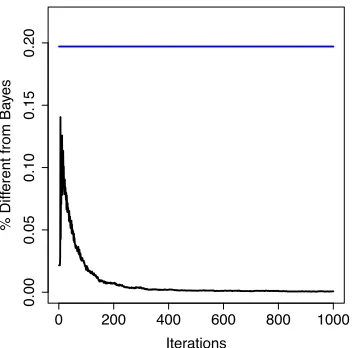
independently on [0,1]20. Figure 8 plots the proportion of points in the hold out sample
classified by AdaBoost as +1 as a function of the number of iterations. This proportion
peaks at.1433 at nine iterations but then gradually decreases to.0175 by 100 iterations and
is equal to .0008 by 1,000 iterations. The fact that by 1,000 iterations only 8 of the 10,000
points in the hold out sample are classified as +1 means there is very little overfitting. The large number of iterations has the effect of smoothing out the classifier resulting in a rule
that agrees with the Bayes rule for 99.92% of the points. Recall that AdaBoost fits the
(a) One-NN (b) AdaBoost
(c) Random Forests (d) CART
Figure 7: Performance of AdaBoost, random forests, and CART on a response surface where
P(y= 1|x) = 0.10 inside the circle and P(y= 1|x)) = 0.90 outside of the circle. There are
0 200 400 600 800 1000
0.00
0.05
0.10
0.15
0.20
Iterations
% Diff
erent from Ba
yes
Figure 8: This plot shows the proportion of points in a test set for which the predictions made by AdaBoost and the Bayes rule differ, as a function of the number of boosting rounds (black). The blue line shows this proportion for the one nearest neighbor classifier. Note that the agreement of AdaBoost and the Bayes rule increases with the number of boosting rounds.
4. Self-Averaging Property of Boosting
4.1 Boosting is Self-Smoothing
In the previous sections, we have demonstrated simple examples where random forests and AdaBoost yield the strongest performance with respect to the Bayes rule. We have argued that these algorithms are successful classifiers due to the fact that they fit initially complex models by interpolating the training data but also exhibit smoothing properties via self-averaging that stabilizes the fit in regions with signal, while continuing to keep localized the effect of noise points on the overall fit. While this smoothing mechanism is obvious for random forests via the averaging over decision trees, it is less obvious for AdaBoost. In this section we explain why the additional iterations in boosting way beyond the point at which perfect classification of the training data (i.e interpolation) has occurred actually has the effect of smoothing out the effects of noise rather than leading to more and more overfitting. To the best of our knowledge, this is a novel perspective on the algorithm. To
explain our key idea, we will recall the pure noise example from before with p=.8,d= 20
and n= 5000.
Recall that the classifier produced by AdaBoost corresponds to I[fM(x)>0] where
fM(x) = M
X
m=1
αmGm(x)
as defined earlier. TakingM = 1000 which was successful in our example let us rewrite
f1000(x) = 1000
X
m=1
αmGm(x) = 10
X
j=1 100
X
k=1
α100(j−1)+kG100(j−1)+k(x) = 10
X
j=1 100
X
k=1 hjk(x)
where
hjk(x)≡α100(j−1)+kG100(j−1)+k(x).
Now define
hjK(x)≡ K
X
k=1 hjk(x)
and note that for every j ∈ {1, ...,10} and every K ∈ {1, ...100} that I[hjK(x) > 0] is
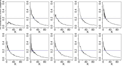
itself a classifier made by linear combinations of classification trees. The ten plots in Figure 9 display the performance on the hold-out sample for these ten classifiers corresponding to
the ten different values forjas a function ofK. Interestingly, each of these 10 classifiers by
itself displays the characteristic of boosting: the agreement with the Bayes rule increases
as more terms are added (for instance, as K is increased).
A second interesting fact about these 10 individual classifiers in the decomposition is that each one achieves perfect separation of the training data and thus each one is an interpolating classifier. This result can be expected in general, provided the total number of iterations for each classifier in the decomposition is sufficiently large. This is clear for the first classifier, since it is simply AdaBoost itself and will necessarily achieve zero training error under some standard conditions as discussed in Jiang (2002). The second classifier in the decomposition is simply AdaBoost weight carried over from the first classifier. Since re-weighting the training data does not prevent AdaBoost from obtaining zero training error, the second classifier also interpolates eventually, as does the third, and so on.
Decomposing boosting in this way offers an explanation of why the additional iterations lead to robustness and better performance in noisy environments rather than severe over-fitting. In this example, AdaBoost for 100 iterations is an interpolating classifier. It makes some errors, mostly near the points in the training data for which the label differs from the Bayes rule, although these are localized. Boosting for 1000 iterations is thus a point-wise weighted average of 10 interpolating classifiers. The random errors near the points in the training data for which the label differ from the Bayes’ rule cancel out in the ensemble av-erage and become even more localized. Of course, the final classifier is still an interpolating classifier as it is an average of 10 interpolating classifiers. In this way, boosting is self-smoothing, self-averaging or self-bagging process that reduces overfitting as the number of iterations increase. The additional iterations provide averaging and smoothing—not over-fitting. Empirically this is very similar to random forests and provides evidence that both algorithms, which perform well in our examples, actually do so using the same mechanism. We further illustrate this phenomenon of increasing localization of the interpolating resulting from this averaging through the following simulation. We take the same training data as before but this time we form the hold out sample by taking a point a (Euclidean)
distance of .1 from each of the 1000 points labeled as−1 in the training data in a random
0 40 80
0.0
0.2
0.4
0.6
K
% Diff
erent from Ba
y
es
0 40 80
0.0
0.2
0.4
0.6
K 0 40 80
0.0
0.2
0.4
0.6
K 0 40 80
0.0
0.2
0.4
0.6
K 0 40 80
0.0
0.2
0.4
0.6
K
0 40 80
0.0
0.2
0.4
0.6
K 0 40 80
0.0
0.2
0.4
0.6
K 0 40 80
0.0
0.2
0.4
0.6
K 0 40 80
0.0
0.2
0.4
0.6
K 0 40 80
0.0
0.2
0.4
0.6
K
Figure 9: A decomposition of boosting
to training set deviations from the Bayes’ rule (points with −1 labels), the error rate is
much higher than it would be for a random sample. However, the interpolation continues to become more localized as the iterations proceed (see Figure 10) so even points that are
quite close to the label errors (the−1 points) eventually become classified correctly as +1.
Comparison to Figure 8 shows that this localization continues at a steady rate even after the error on the random hold-out sample is practically zero. In contrast, the nearest neighbor interpolator this simulation yielded 100% disagreement with the Bayes’ rule.
4.2 A Five-Dimensional Example
We will now consider a second simulation to further illustrate how this self-averaging prop-erty of AdaBoost helps prevent overfitting and improves performance. In this simulation
we add signal while retaining significant random noise. Let n= 400,d= 5 and sample xi
distributed iiduniform on [0,1]5. The true model from for the simulation is
P(y= 1|x) =.2 +.6
I
2
X
j=1 xj >1
.
The Bayes’ error is 0.20 and the optimal Bayes’ decision boundary is the diagonal of the
unit square in x1 and x2. Even with this small sample size, AdaBoost interpolates the
0 200 400 600 800 1000
0.00
0.05
0.10
0.15
0.20
0.25
0.30
0.35
Iterations
% Diff
erent from Ba
y
es
Figure 10: This plot shows the proportion of points in a test set for which the predictions made by AdaBoost and the Bayes rule differ, as a function of the number of boosting rounds (black). The test set has been chosen to contain excess points near the error points in the training set.
sets of ten (which is analogous to the 10 sets of 100 from the 20 dimensional example in the previous section).
The ten plots in the first two rows in Figure 11 show the performance of the ten classifiers corresponding to this decomposition with respect to a hold out sample of 1000 points. Each point in the figure represents a point classified differently from the Bayes rule. While each of the ten classifiers in the decomposition classifies a number of these 1000 points incorrectly especially along the Bayes boundary, exactly which points are classified incorrectly varies considerably from one classifier to the next. The final classifier (displayed in the last plot), which corresponds to AdaBoost after 100 iterations, makes fewer mistakes than each of the ten individual classifiers. Since AdaBoost is a point-wise weighted average of the 10 classifiers, the averaging over the highly variable error locations made by each classifier reduces substantially the number of errors made by the ensemble. The percentage of points classified differently from the Bayes’ rule by the final classifier is 118/1000=0.118 while after the first ten there were still 162/1000=0.162 classified differently from the Bayes rule. Averaged over 200 repetitions of this simulation these numbers are .19 after the first ten iterations and .15 after 100 iterations confirming that the performance does improve by running beyond the point at which interpolation initially occurs as (a result of this self-smoothing).
In this example, we also have evidence that AdaBoost takes some measure to decorrelate the errors made by its base classifiers, as hypothesized in Amit et al. (2000) and suggested in
Figure 11. To this end, we computed the correlation betweenI[h110(X) =Y], . . . ,I[h1010(X) =
Y] over a large test set. The correlations ranged from 0.4 to 0.56, with an average value
● ● ● ● ● ● ● ● ● ● ● ● ● ● ● ● ● ● ● ● ● ● ● ● ● ● ● ● ● ● ● ● ● ● ● ● ● ● ● ● ● ● ● ● ● ● ● ● ● ● ● ● ● ● ● ● ● ● ● ● ● ● ● ● ● ● ● ● ● ● ● ● ● ● ● ● ● ● ● ● ● ● ● ● ● ● ● ● ● ● ● ● ● ● ● ● ● ● ● ● ● ● ● ● ● ● ● ● ● ● ● ● ● ● ● ● ● ● ● ● ● ● ● ● ● ● ● ● ● ● ● ● ● ● ● ● ● ● ● ● ● ● ● ● ● ● ● ● ● ● ● ● ● ● ● ● ● ● ● ● ● ●
0.0 0.4 0.8
0.0 0.4 0.8 ● ● ● ● ● ● ● ● ● ● ● ● ● ● ● ● ● ● ● ● ● ● ● ● ● ● ● ● ● ● ● ● ● ● ● ● ● ● ● ● ● ● ● ● ● ● ● ● ● ● ● ● ● ● ● ● ● ● ● ● ● ● ● ● ● ● ● ● ● ● ● ● ● ● ● ● ● ● ● ● ● ● ● ● ● ● ● ● ● ● ● ● ● ● ● ● ● ● ● ●● ● ● ● ● ● ● ● ● ● ● ● ● ● ● ● ● ● ●● ● ● ● ● ● ● ● ● ● ● ● ● ● ● ● ● ● ● ● ● ● ● ● ● ● ● ● ● ● ● ● ● ● ● ● ● ● ● ● ● ● ● ● ● ● ●
0.0 0.4 0.8
0.0 0.4 0.8 ● ● ● ● ● ● ● ● ● ● ● ● ● ● ● ● ● ● ● ● ● ● ● ● ● ● ● ● ● ● ● ● ● ● ● ● ● ● ● ● ● ● ● ● ● ● ● ● ● ● ● ● ● ● ● ● ● ● ● ● ● ● ● ● ● ● ● ● ● ● ● ● ● ● ● ● ● ● ● ● ● ● ● ● ● ● ● ● ● ● ● ● ● ● ● ● ● ● ● ● ● ● ● ● ● ● ● ● ● ● ● ● ● ● ● ● ● ● ● ● ● ● ● ● ● ● ● ● ● ● ●● ● ● ● ● ● ● ● ● ● ● ● ● ● ● ● ● ● ● ● ● ● ● ● ● ● ● ● ● ● ● ● ● ● ● ● ● ● ● ●
0.0 0.4 0.8
0.0 0.4 0.8 ● ● ● ● ● ● ● ● ● ● ● ● ● ● ● ● ● ● ● ● ● ● ● ● ● ● ● ● ● ● ● ● ● ● ● ● ● ● ● ● ● ● ● ● ● ● ● ● ● ● ● ● ● ● ● ● ● ● ● ● ● ● ● ● ● ● ● ● ● ● ● ● ● ● ● ● ● ● ● ● ● ● ● ● ● ● ● ●● ●● ● ● ● ● ● ● ● ● ● ● ● ● ● ● ● ● ● ● ● ● ● ● ● ● ● ● ● ● ● ● ● ● ● ● ● ● ● ● ● ● ● ● ● ● ● ● ● ● ● ● ● ● ● ● ● ● ● ● ● ● ● ● ● ● ● ● ● ● ● ● ● ● ● ● ● ● ● ● ● ● ● ● ● ●
0.0 0.4 0.8
0.0 0.4 0.8 ● ● ● ● ● ● ● ● ● ● ● ● ● ● ● ● ● ● ● ● ● ● ● ● ● ● ● ● ● ● ● ● ● ● ● ● ● ● ● ● ● ● ● ● ● ● ● ● ● ● ● ● ● ● ● ● ● ● ● ● ● ● ● ● ● ● ● ● ● ● ● ● ● ● ● ● ● ● ● ● ● ● ● ● ● ● ● ● ● ● ● ●● ● ● ● ● ● ● ● ● ● ● ● ● ● ● ● ● ● ● ● ● ● ● ● ● ●● ● ● ● ● ● ● ● ● ● ● ● ● ● ● ● ● ● ● ● ● ● ● ● ● ● ● ● ● ● ● ● ● ● ● ● ● ● ● ● ● ● ● ● ● ● ● ● ● ● ● ● ● ● ● ●● ● ● ● ● ● ● ● ● ● ● ● ● ● ● ●
0.0 0.4 0.8
0.0 0.4 0.8 ● ● ● ● ● ● ● ● ● ● ● ● ● ● ● ● ● ● ● ● ● ● ● ● ● ● ● ● ● ● ● ● ● ● ● ● ● ● ● ● ● ● ● ● ● ● ● ● ● ● ● ● ●● ● ● ● ● ● ● ● ● ● ● ● ● ● ● ● ● ● ● ● ● ● ● ● ● ● ● ● ● ● ● ● ● ● ● ● ● ● ● ● ● ● ● ● ● ● ● ● ● ● ● ● ● ● ● ● ● ● ● ● ● ● ● ● ● ● ● ● ● ● ● ● ● ● ● ● ● ● ● ● ● ● ● ● ● ● ● ● ● ● ● ● ● ● ● ● ● ● ● ● ● ● ● ● ● ● ● ● ● ● ● ● ● ● ● ● ● ● ● ● ● ● ● ● ● ● ● ● ● ● ● ● ● ● ● ● ● ● ● ● ● ● ● ● ● ● ● ● ● ● ● ● ● ● ● ● ● ● ● ● ● ● ● ● ● ● ● ● ● ● ● ● ●● ● ● ● ● ● ● ●
0.0 0.4 0.8
0.0 0.4 0.8 ● ● ● ● ● ● ● ● ● ● ● ● ● ● ● ● ● ● ● ● ● ● ● ● ● ● ● ● ● ● ● ● ● ● ● ● ● ● ● ● ● ● ● ● ● ● ● ● ● ● ● ● ● ● ● ● ● ● ● ● ● ● ● ● ● ● ● ● ● ● ● ● ● ● ● ● ● ● ● ● ● ● ● ● ● ● ● ● ● ● ● ● ● ● ● ● ● ● ● ● ● ● ● ● ● ● ● ● ● ● ● ● ● ● ● ● ● ● ● ● ●● ● ● ● ● ● ● ● ● ● ● ● ● ● ● ● ● ● ● ● ● ● ● ● ● ● ● ● ● ● ● ● ● ● ● ● ● ● ● ● ● ● ● ● ● ● ● ● ● ● ● ● ● ● ● ● ● ● ● ● ● ● ● ● ● ● ● ● ● ● ● ● ● ● ● ● ● ● ●
0.0 0.4 0.8
0.0 0.4 0.8 ● ● ● ● ● ● ● ● ● ● ● ● ● ● ● ● ● ● ● ● ● ● ● ● ● ● ● ● ● ● ● ● ● ● ● ● ● ● ● ● ● ● ● ● ● ● ● ● ● ● ● ● ● ● ● ● ● ● ● ● ● ● ● ● ● ● ● ● ● ● ● ● ● ● ● ● ● ● ● ● ● ● ● ● ● ● ● ● ● ● ● ● ● ● ● ● ● ● ● ● ● ● ● ● ● ● ● ● ● ● ● ● ● ● ● ● ● ● ● ● ● ● ● ● ● ● ● ● ● ● ● ● ● ● ● ● ● ● ● ● ● ● ● ● ● ● ● ● ●● ● ● ● ● ● ● ● ● ● ● ● ● ● ● ● ● ● ● ● ● ● ● ● ● ● ● ● ● ● ● ● ● ● ● ● ● ● ● ● ● ● ● ● ● ● ●
0.0 0.4 0.8
0.0 0.4 0.8 ● ● ● ● ● ● ● ● ● ● ● ● ● ● ● ● ● ● ● ● ● ● ● ● ● ● ● ● ● ● ● ● ● ● ● ● ● ● ● ● ● ● ● ● ● ● ● ● ● ● ● ● ● ● ● ● ● ● ● ● ● ● ● ● ● ● ● ● ● ● ● ● ● ● ● ● ● ● ● ● ● ● ● ● ● ● ● ● ● ● ● ● ● ● ● ● ● ● ● ● ● ● ● ● ● ● ● ● ● ● ● ● ● ● ● ● ● ● ● ● ● ● ● ● ● ● ● ● ● ● ● ● ● ● ● ● ● ● ● ● ● ● ● ● ● ● ● ● ● ● ● ● ● ● ● ● ● ● ● ● ● ● ● ●● ● ● ● ●
0.0 0.4 0.8
0.0 0.4 0.8 ● ● ● ● ● ● ● ● ● ● ● ● ● ● ● ● ● ● ● ● ● ● ● ● ● ● ● ● ● ● ● ● ● ● ● ● ● ● ● ● ● ● ● ● ● ● ● ● ● ● ● ● ● ● ● ● ● ● ● ● ● ● ● ● ● ● ● ● ● ● ● ● ● ● ● ● ● ● ● ● ● ● ● ● ● ● ● ● ● ● ● ● ● ● ● ● ● ● ● ● ● ● ● ● ● ● ● ● ● ● ● ● ● ● ● ● ● ● ● ● ● ● ● ● ● ● ● ● ● ● ● ● ● ● ● ● ● ● ● ● ● ● ● ● ● ● ● ● ● ● ● ● ● ● ● ● ● ● ● ● ● ● ● ● ● ● ●● ● ● ● ● ● ● ● ● ● ● ● ● ● ● ● ● ● ● ● ● ● ● ● ● ● ● ● ● ● ● ● ● ● ● ● ● ● ● ● ● ● ● ● ● ● ● ● ● ● ● ● ●
0.0 0.4 0.8
0.0 0.4 0.8 ● ● ● ● ● ● ● ● ● ● ● ● ● ● ● ● ● ● ● ● ● ● ● ● ● ● ● ● ● ● ● ● ● ● ● ● ● ● ● ● ● ● ● ● ● ● ● ● ● ● ● ●● ● ● ● ● ● ● ● ● ● ● ● ● ● ● ● ● ● ● ● ● ● ● ● ● ● ● ● ● ● ● ● ● ● ● ● ● ● ● ● ● ● ● ● ● ● ● ● ● ● ● ● ● ● ● ● ● ● ● ● ● ● ●
0.0 0.4 0.8
0.0
0.4
0.8
sub-ensembles of 20 trees in the case of the random forest, and 10 sub-ensembles of trees in the case of bagged trees. The interpolating classifiers produced by the random forest had error correlations ranging from 0.75 to 0.87, with an average of 0.81, while the correlations for the bagged trees ranged from 0.9 to 0.94, with an average value of 0.92. In other words, the sub-ensembles produced by random forests and AdaBoost are less correlated than the bagged trees, with AdaBoost being markedly less so. When voting across constituents in its decomposition, it is clear that such a decorrelating effect would help to increase the effectiveness of the voting mechanism to cancel out error points. While we observed this phenomenon in a few data sets, we cannot state under what conditions it happens more generally. However, it is know that boosting generally outperforms bagging, and that bagged trees will be much more correlated.
4.3 Comparison to Boosted Stumps
Throughout this paper we have considered AdaBoost with large trees of up to 28 terminal
nodes. We have shown that AdaBoost with such large trees is a classifier which interpolates the data in such a way that it performs well out of sample for problems in which the Bayes’ error rate is substantially larger than zero. In this section we will consider the performance of AdaBoost with stumps as the base learner. The statistical theory predicts that AdaBoost with stumps will overfit less than AdaBoost with larger trees, as expressed, for instance, in Jiang (2002). It is also thought that stumps should be preferable when the Bayes’ decision rule is additive in the original predictors. For instance the seminal book by Hastie et al. (2009, chapter 10) advocates using trees of a depth one greater than the dominant level of interaction, which is generally quite low.
AdaBoost with stumps does not self-smooth nearly as well as with larger trees, likely because the the classifiers in the decomposition are more highly correlated, and the “rough” fits from stumps fail to interpolate the training data locally enough; the fit is not spiked-smooth around the training set error points. Consequently, AdaBoost with stumps as base learners is outperformed by AdaBoost with large trees as base learners, when the Bayes error rate is high. This is the case even when the Bayes rule is additive. This result is matched by random forests which works best with large trees. Its randomly chosen predictors at each splitting opportunity lowers the correlation among the trees and the resulting fit is more spiked-smooth.
To illustrate this with an example, we return to the five dimensional simulation from Section 4.2 which has an additive Bayes decision rule. Figure 12 displays the percentage of points that are classified differently from the Bayes rule in the hold out sample of 1000, as a function of the number of iterations. It can be seen that the stumps (left panel) do
not perform as well as the 28 node trees (right panel). After 250 iterations, AdaBoost
with stumps yields 141/1000 points in the hold out sample classified differently from the
Bayes rule, compared to 116/1000 for this same data set using instead AdaBoost with 28
node trees. In fact, the stumps seems to suffer from overfitting when run beyond only
25 iterations, while the 28 trees do not have a problem with overfitting as the number of
iterations are increased.
0 50 100 150 200 250
0.10
0.15
0.20
0.25
0.30
Iterations
% Diff
erent from Ba
yes
(a) Stump
0 50 100 150 200 250
0.10
0.15
0.20
0.25
0.30
Iterations
% Diff
erent from Ba
yes
(b) 28 Node Trees
Figure 12: Comparison of AdaBoost with stumps (a) and 28 node trees (b) for the five
dimensional simulation. The blue line corresponds to One-NN.
good out-of-sample performance of AdaBoost using large trees resulting from the local in-terpolation of noise points is not shared by AdaBoost using stumps. The idea that stumps will perform better in noisy environments because they overfit less is not supported by this simulation. While the stumps do overfit less on the training data, as evidenced by the fact that they did not give zero training error, they actually overfit worse than the larger trees out of sample. Again, we attribute this to boosting with stumps lacking the self-smoothing property and not being flexible enough to interpolate the noise locally.
5. Real Data Example
In previous sections, we explored the mechanism of spiked smoothing in simulation exper-iments where it was easy for us to identify noise points. Recall that with a fully specified probability model, noise points are simply sample points whose sign differs from the Bayes’ rule. While simulated examples are certainly good for illustration, one may wonder whether these settings are overly simplistic. Data in the real world is typically generated by more complicated—and unknown—probability models with heteroskedastic noise components. Since boosted trees have been empirically successful in such settings, it pays to move our discussion to the context of a data set arising in the real world.
5.1 Phoneme Data
language 2. For a collection of 5404 examples of spoken vowels, this data set contains the amplitudes of the first 5 harmonic frequencies as collected by a cochlea spectra (hearing aid), along with a label of either nasal or oral (n=5404, p=5). The goal is then to use these harmonic frequencies to correctly identify the type of vowel. While there are many potential data sets we could have considered, this one is convenient to analyze since it consists of a relatively small number of real valued covariates. This makes it easier to talk about “neighborhoods” of points later in our discussion.
We begin by dividing the phoneme data set up into a training set consisting of 70% of the samples, and a testing set consisting of 30% of the examples. Depth eight decision trees boosted for 1000 rounds and a random forest classifier both achieve comparable test error
rates of 9.0% and 9.4%, respectively 3. Figure 13 demonstrates that boosting deep trees is
preferable to shallow trees in this data set. Each frame in the figure shows the testing error in black and the training error in red as a function of the number of boosting iterations for different depth trees. One can readily observe that test error steadily decreases with the depth of tree used in AdaBoost. It is interesting to note that boosting trees of all depths are slow to overfit the data, even with boosted stumps after 1000 iterations. It is also worth noting that boosted depth 8 trees quickly interpolate the training data, as indicated by the sharply decreasing red line. This raises the often asked question: what is AdaBoost doing after it achieves a perfect fit on the training set?
Any discussion of spiked smoothing on real data is complicated by the reality that it is impossible to identify noise points without knowing the underlying probability model. As a substitute for noise points, we flipped the signs of 100 randomly chosen points in our training data set (about 2% of the data) and analyzed the fits of boosted trees and a random forest classifier around these points. After refitting the models to the perturbed data, we find the the testing errors are 10.2% and 10.0% for boosted depth eight trees and a random forest, respectively. Figure 14 illustrates that even after thousands of rounds of boosting, test error continues to decrease. The punchline is that both algorithms are able to achieve fits with comparable test set error even after flipping the sign of a large number of points in the training set.
As a comparison with another interpolating classifier, we also repeated the same experi-ment with a one nearest-neighbors classifier. We found the one nearest neighbor achieved a test error rate of 10.5% when fit on the original training set, and a test error rate of 12.6% when fit on the noisy training set. The increase in error rate when noise is added to the training set is larger than that of AdaBoost or a random forest, which coincides with the results form the simulated example in section 3.3. Furthermore, two sample t-tests reveal that the increase in error rate for one nearest-neighbors is significant at the 0.01 level in
both cases (p-values less than 1e−16 in both cases).
We will argue that additional rounds of boosting are helping to “smooth out” and “localize” the influence of the 100 noise points that we introduced into our training set. In section 3.3, we illustrated the action of spiked smoothing in diagrams which showed AdaBoost’s fit on a two dimensional plane. In this slightly higher dimensional example,
2. The original data can be found at the following address:
https://www.elen.ucl.ac.be/neural-nets/Research/Projects/ELENA/databases/REAL/phoneme/phoneme.txt.
0.05 0.10 0.15 0.20 0.25
0 250 500 750 1000 Iterations
Error
Tree Depth: 1
0.05 0.10 0.15 0.20 0.25
0 250 500 750 1000
Tree Depth: 5
0.05 0.10 0.15 0.20 0.25
0 250 500 750 1000
Tree Depth: 2
0.05 0.10 0.15 0.20 0.25
0 250 500 750 1000
Tree Depth: 6
0.05 0.10 0.15 0.20 0.25
0 250 500 750 1000
Tree Depth: 3
0.05 0.10 0.15 0.20 0.25
0 250 500 750 1000
Tree Depth: 7
0.05 0.10 0.15 0.20 0.25
0 250 500 750 1000
Tree Depth: 4
0.05 0.10 0.15 0.20 0.25
0 250 500 750 1000
Tree Depth: 8
Figure 13: Plots of testing and training error as a function of number of boosting iterations for trees of different depths. The black lines show the test error rates while the red lines show training error rates. Notice that depth seven and eight boosted trees quickly fit the training data, as depicted by the rapidly decreasing red lines.
0.12 0.14 0.16
0 1000 2000 3000
Iterations
T
est Error
Figure 14: Plot of testing error for depth 8 boosted trees fit to a training set which has flipped labels for 100 randomly selected examples.