Data Structures
and Algorithm
Analysis in
Data Structures
and Algorithm
Analysis in
C
++
M a r k A l l e n W e i s s
Florida International University
Boston Columbus Indianapolis New York San Francisco
Upper Saddle River Amsterdam Cape Town Dubai London
Madrid Milan Munich Paris Montreal Toronto Delhi
Mexico City Sao Paulo Sydney Hong Kong Seoul Singapore
Editorial Assistant: Jenah Blitz-Stoehr Permissions Administrator: Jenell Forschler Director of Marketing: Christy Lesko Cover Image: cDe-kay | Dreamstime.com Marketing Manager: Yez Alayan Media Project Manager: Renata Butera
Senior Marketing Coordinator: Kathryn Ferranti Full-Service Project Management: Integra Software Marketing Assistant: Jon Bryant Services Pvt. Ltd.
Director of Production: Erin Gregg Composition: Integra Software Services Pvt. Ltd. Senior Managing Editor: Scott Disanno Text and Cover Printer/Binder: Courier Westford Senior Production Project Manager: Marilyn Lloyd
Manufacturing Buyer: Linda Sager Art Director: Jayne Conte
Copyright c2014, 2006, 1999 Pearson Education, Inc., publishing as Addison-Wesley. All rights reserved. Printed in the United States of America. This publication is protected by Copyright, and permission should be obtained from the publisher prior to any prohibited reproduction, storage in a retrieval system, or transmission in any form or by any means, electronic, mechanical, photocopying, recording, or likewise. To obtain permission(s) to use material from this work, please submit a written request to Pearson Education, Inc., Permissions Department, One Lake Street, Upper Saddle River, New Jersey 07458, or you may fax your request to 201-236-3290.
Many of the designations by manufacturers and sellers to distinguish their products are claimed as trademarks. Where those designations appear in this book, and the publisher was aware of a trademark claim, the designations have been printed in initial caps or all caps.
Library of Congress Cataloging-in-Publication Data
Weiss, Mark Allen.
Data structures and algorithm analysis in C++ / Mark Allen Weiss, Florida International University. — Fourth edition.
pages cm
ISBN-13: 978-0-13-284737-7 (alk. paper) ISBN-10: 0-13-284737-X (alk. paper)
1. C++ (Computer program language) 2. Data structures (Computer science) 3. Computer algorithms. I. Title. QA76.73.C153W46 2014
005.73—dc23
2013011064
10 9 8 7 6 5 4 3 2 1
www.pearsonhighered.com
Preface xv
Chapter 1 Programming: A General Overview
1
1.1 What’s This Book About? 11.2 Mathematics Review 2 1.2.1 Exponents 3 1.2.2 Logarithms 3 1.2.3 Series 4
1.2.4 Modular Arithmetic 5 1.2.5 ThePWord 6
1.3 A Brief Introduction to Recursion 8 1.4 C++ Classes 12
1.4.1 BasicclassSyntax 12
1.4.2 Extra Constructor Syntax and Accessors 13 1.4.3 Separation of Interface and Implementation 16 1.4.4 vectorandstring 19
1.5 C++ Details 21 1.5.1 Pointers 21
1.5.2 Lvalues, Rvalues, and References 23 1.5.3 Parameter Passing 25
1.5.4 Return Passing 27
1.5.5 std::swapandstd::move 29
1.5.6 The Big-Five: Destructor, Copy Constructor, Move Constructor, Copy Assignmentoperator=, Move Assignmentoperator= 30
1.5.7 C-style Arrays and Strings 35 1.6 Templates 36
1.6.1 Function Templates 37 1.6.2 Class Templates 38
1.6.3 Object,Comparable, and an Example 39 1.6.4 Function Objects 41
1.6.5 Separate Compilation of Class Templates 44 1.7 Using Matrices 44
1.7.1 The Data Members, Constructor, and Basic Accessors 44 1.7.2 operator[] 45
1.7.3 Big-Five 46 Summary 46 Exercises 46 References 48
Chapter 2 Algorithm Analysis
51
2.1 Mathematical Background 51 2.2 Model 54
2.3 What to Analyze 54
2.4 Running-Time Calculations 57 2.4.1 A Simple Example 58 2.4.2 General Rules 58
2.4.3 Solutions for the Maximum Subsequence Sum Problem 60
2.4.4 Logarithms in the Running Time 66 2.4.5 Limitations of Worst-Case Analysis 70 Summary 70
Exercises 71 References 76
Chapter 3 Lists, Stacks, and Queues
77
3.1 Abstract Data Types (ADTs) 773.2 The List ADT 78
3.2.1 Simple Array Implementation of Lists 78 3.2.2 Simple Linked Lists 79
3.3 vectorandlistin the STL 80
3.3.1 Iterators 82
3.3.2 Example: Usingeraseon a List 83 3.3.3 const_iterators 84
3.4 Implementation ofvector 86 3.5 Implementation oflist 91 3.6 The Stack ADT 103
3.6.1 Stack Model 103
3.6.2 Implementation of Stacks 104 3.6.3 Applications 104
3.7 The Queue ADT 112 3.7.1 Queue Model 113
3.7.2 Array Implementation of Queues 113 3.7.3 Applications of Queues 115
Chapter 4 Trees
121
4.1 Preliminaries 1214.1.1 Implementation of Trees 122
4.1.2 Tree Traversals with an Application 123 4.2 Binary Trees 126
4.2.1 Implementation 128
4.2.2 An Example: Expression Trees 128 4.3 The Search Tree ADT—Binary Search Trees 132
4.3.1 contains 134
4.3.2 findMinandfindMax 135 4.3.3 insert 136
4.3.4 remove 139
4.3.5 Destructor and Copy Constructor 141 4.3.6 Average-Case Analysis 141
4.4 AVL Trees 144
4.4.1 Single Rotation 147 4.4.2 Double Rotation 149 4.5 Splay Trees 158
4.5.1 A Simple Idea (That Does Not Work) 158 4.5.2 Splaying 160
4.6 Tree Traversals (Revisited) 166 4.7 B-Trees 168
4.8 Sets and Maps in the Standard Library 173 4.8.1 Sets 173
4.8.2 Maps 174
4.8.3 Implementation ofset and map 175 4.8.4 An Example That Uses Several Maps 176 Summary 181
Exercises 182 References 189
Chapter 5 Hashing
193
5.1 General Idea 193 5.2 Hash Function 194 5.3 Separate Chaining 196
5.4 Hash Tables without Linked Lists 201 5.4.1 Linear Probing 201
5.4.2 Quadratic Probing 202 5.4.3 Double Hashing 207 5.5 Rehashing 208
5.7 Hash Tables with Worst-CaseO(1) Access 212 5.7.1 Perfect Hashing 213
5.7.2 Cuckoo Hashing 215 5.7.3 Hopscotch Hashing 227 5.8 Universal Hashing 230 5.9 Extendible Hashing 233
Summary 236 Exercises 237 References 241
Chapter 6 Priority Queues (Heaps)
245
6.1 Model 2456.2 Simple Implementations 246 6.3 Binary Heap 247
6.3.1 Structure Property 247 6.3.2 Heap-Order Property 248 6.3.3 Basic Heap Operations 249 6.3.4 Other Heap Operations 252 6.4 Applications of Priority Queues 257
6.4.1 The Selection Problem 258 6.4.2 Event Simulation 259 6.5 d-Heaps 260
6.6 Leftist Heaps 261
6.6.1 Leftist Heap Property 261 6.6.2 Leftist Heap Operations 262 6.7 Skew Heaps 269
6.8 Binomial Queues 271
6.8.1 Binomial Queue Structure 271 6.8.2 Binomial Queue Operations 271
6.8.3 Implementation of Binomial Queues 276 6.9 Priority Queues in the Standard Library 282
Summary 283 Exercises 283 References 288
Chapter 7 Sorting
291
7.1 Preliminaries 291 7.2 Insertion Sort 292
7.2.1 The Algorithm 292
7.2.2 STL Implementation of Insertion Sort 293 7.2.3 Analysis of Insertion Sort 294
7.4 Shellsort 296
7.4.1 Worst-Case Analysis of Shellsort 297 7.5 Heapsort 300
7.5.1 Analysis of Heapsort 301 7.6 Mergesort 304
7.6.1 Analysis of Mergesort 306 7.7 Quicksort 309
7.7.1 Picking the Pivot 311 7.7.2 Partitioning Strategy 313 7.7.3 Small Arrays 315
7.7.4 Actual Quicksort Routines 315 7.7.5 Analysis of Quicksort 318
7.7.6 A Linear-Expected-Time Algorithm for Selection 321 7.8 A General Lower Bound for Sorting 323
7.8.1 Decision Trees 323
7.9 Decision-Tree Lower Bounds for Selection Problems 325 7.10 Adversary Lower Bounds 328
7.11 Linear-Time Sorts: Bucket Sort and Radix Sort 331 7.12 External Sorting 336
7.12.1 Why We Need New Algorithms 336 7.12.2 Model for External Sorting 336 7.12.3 The Simple Algorithm 337 7.12.4 Multiway Merge 338 7.12.5 Polyphase Merge 339 7.12.6 Replacement Selection 340 Summary 341
Exercises 341 References 347
Chapter 8 The Disjoint Sets Class
351
8.1 Equivalence Relations 3518.2 The Dynamic Equivalence Problem 352 8.3 Basic Data Structure 353
8.4 Smart Union Algorithms 357 8.5 Path Compression 360
8.6 Worst Case for Union-by-Rank and Path Compression 361 8.6.1 Slowly Growing Functions 362
8.6.2 An Analysis by Recursive Decomposition 362 8.6.3 AnO(Mlog *N) Bound 369
Summary 374 Exercises 375 References 376
Chapter 9 Graph Algorithms
379
9.1 Definitions 379
9.1.1 Representation of Graphs 380 9.2 Topological Sort 382
9.3 Shortest-Path Algorithms 386 9.3.1 Unweighted Shortest Paths 387 9.3.2 Dijkstra’s Algorithm 391
9.3.3 Graphs with Negative Edge Costs 400 9.3.4 Acyclic Graphs 400
9.3.5 All-Pairs Shortest Path 404 9.3.6 Shortest Path Example 404 9.4 Network Flow Problems 406
9.4.1 A Simple Maximum-Flow Algorithm 408 9.5 Minimum Spanning Tree 413
9.5.1 Prim’s Algorithm 414 9.5.2 Kruskal’s Algorithm 417
9.6 Applications of Depth-First Search 419 9.6.1 Undirected Graphs 420
9.6.2 Biconnectivity 421 9.6.3 Euler Circuits 425 9.6.4 Directed Graphs 429
9.6.5 Finding Strong Components 431 9.7 Introduction to NP-Completeness 432
9.7.1 Easy vs. Hard 433 9.7.2 The Class NP 434
9.7.3 NP-Complete Problems 434 Summary 437
Exercises 437 References 445
Chapter 10 Algorithm Design Techniques
449
10.1 Greedy Algorithms 44910.1.1 A Simple Scheduling Problem 450 10.1.2 Huffman Codes 453
10.1.3 Approximate Bin Packing 459 10.2 Divide and Conquer 467
10.2.3 The Selection Problem 475
10.2.4 Theoretical Improvements for Arithmetic Problems 478 10.3 Dynamic Programming 482
10.3.1 Using a Table Instead of Recursion 483 10.3.2 Ordering Matrix Multiplications 485 10.3.3 Optimal Binary Search Tree 487 10.3.4 All-Pairs Shortest Path 491 10.4 Randomized Algorithms 494
10.4.1 Random-Number Generators 495 10.4.2 Skip Lists 500
10.4.3 Primality Testing 503 10.5 Backtracking Algorithms 506
10.5.1 The Turnpike Reconstruction Problem 506 10.5.2 Games 511
Summary 518 Exercises 518 References 527
Chapter 11 Amortized Analysis
533
11.1 An Unrelated Puzzle 53411.2 Binomial Queues 534 11.3 Skew Heaps 539 11.4 Fibonacci Heaps 541
11.4.1 Cutting Nodes in Leftist Heaps 542 11.4.2 Lazy Merging for Binomial Queues 544 11.4.3 The Fibonacci Heap Operations 548 11.4.4 Proof of the Time Bound 549 11.5 Splay Trees 551
Summary 555 Exercises 556 References 557
Chapter 12 Advanced Data Structures
and Implementation
559
12.1 Top-Down Splay Trees 559 12.2 Red-Black Trees 566
12.4 Suffix Arrays and Suffix Trees 579 12.4.1 Suffix Arrays 580
12.4.2 Suffix Trees 583
12.4.3 Linear-Time Construction of Suffix Arrays and Suffix Trees 586 12.5k-d Trees 596
12.6 Pairing Heaps 602 Summary 606 Exercises 608 References 612
Appendix A Separate Compilation of
Class Templates
615
A.1 Everything in the Header 616 A.2 Explicit Instantiation 616
Purpose/Goals
The fourth edition ofData Structures and Algorithm Analysis in C++describesdata structures, methods of organizing large amounts of data, andalgorithm analysis,the estimation of the running time of algorithms. As computers become faster and faster, the need for programs that can handle large amounts of input becomes more acute. Paradoxically, this requires more careful attention to efficiency, since inefficiencies in programs become most obvious when input sizes are large. By analyzing an algorithm before it is actually coded, students can decide if a particular solution will be feasible. For example, in this text students look at specific problems and see how careful implementations can reduce the time constraint for large amounts of data from centuries to less than a second. Therefore, no algorithm or data structure is presented without an explanation of its running time. In some cases, minute details that affect the running time of the implementation are explored.
Once a solution method is determined, a program must still be written. As computers have become more powerful, the problems they must solve have become larger and more complex, requiring development of more intricate programs. The goal of this text is to teach students good programming and algorithm analysis skills simultaneously so that they can develop such programs with the maximum amount of efficiency.
This book is suitable for either an advanced data structures course or a first-year graduate course in algorithm analysis. Students should have some knowledge of inter-mediate programming, including such topics as pointers, recursion, and object-based programming, as well as some background in discrete math.
Approach
Although the material in this text is largely language-independent, programming requires the use of a specific language. As the title implies, we have chosen C++ for this book.
C++ has become a leading systems programming language. In addition to fixing many of the syntactic flaws of C, C++ provides direct constructs (the class and template) to implement generic data structures as abstract data types.
The most difficult part of writing this book was deciding on the amount of C++ to include. Use too many features of C++ and one gets an incomprehensible text; use too few and you have little more than a C text that supports classes.
The approach we take is to present the material in anobject-based approach.As such, there is almost no use of inheritance in the text. We use class templates to describe generic data structures. We generally avoid esoteric C++ features and use thevectorand string classes that are now part of the C++ standard. Previous editions have implemented class templates by separating the class template interface from its implementation. Although
difficult for readers to actually use the code. As a result, in this edition the online code represents class templates as a single unit, with no separation of interface and implementa-tion. Chapter 1 provides a review of the C++ features that are used throughout the text and describes our approach to class templates. Appendix A describes how the class templates could be rewritten to use separate compilation.
Complete versions of the data structures, in both C++ and Java, are available on the Internet. We use similar coding conventions to make the parallels between the two languages more evident.
Summary of the Most Significant Changes in the Fourth Edition
The fourth edition incorporates numerous bug fixes, and many parts of the book have undergone revision to increase the clarity of presentation. In addition,
r Chapter 4 includes implementation of the AVL tree deletion algorithm—a topic often requested by readers.
r Chapter 5 has been extensively revised and enlarged and now contains material on two newer algorithms: cuckoo hashing and hopscotch hashing. Additionally, a new section on universal hashing has been added. Also new is a brief discussion of the unordered_setandunordered_mapclass templates introduced in C++11.
r Chapter 6 is mostly unchanged; however, the implementation of the binary heap makes use of move operations that were introduced in C++11.
r Chapter 7 now contains material on radix sort, and a new section on lower-bound proofs has been added. Sorting code makes use of move operations that were introduced in C++11.
r Chapter 8 uses the new union/find analysis by Seidel and Sharir and shows the O(Mα(M,N) ) bound instead of the weakerO(Mlog∗N) bound in prior editions. r Chapter 12 adds material on suffix trees and suffix arrays, including the linear-time
suffix array construction algorithm by Karkkainen and Sanders (with implementation). The sections covering deterministic skip lists and AA-trees have been removed. r Throughout the text, the code has been updated to use C++11. Notably, this means
use of the new C++11 features, including theautokeyword, the rangeforloop, move construction and assignment, and uniform initialization.
Overview
Chapter 1 contains review material on discrete math and recursion. I believe the only way to be comfortable with recursion is to see good uses over and over. Therefore, recursion is prevalent in this text, with examples in every chapter except Chapter 5. Chapter 1 also includes material that serves as a review of basic C++. Included is a discussion of templates and important constructs in C++ class design.
Chapter 3 covers lists, stacks, and queues. This chapter includes a discussion of the STL vectorandlistclasses, including material on iterators, and it provides implementations of a significant subset of theSTL vector and listclasses.
Chapter 4 covers trees, with an emphasis on search trees, including external search trees (B-trees). TheUNIXfile system and expression trees are used as examples. AVL trees and splay trees are introduced. More careful treatment of search tree implementation details is found in Chapter 12. Additional coverage of trees, such as file compression and game trees, is deferred until Chapter 10. Data structures for an external medium are considered as the final topic in several chapters. Included is a discussion of the STLsetandmapclasses, including a significant example that illustrates the use of three separate maps to efficiently solve a problem.
Chapter 5 discusses hash tables, including the classic algorithms such as sepa-rate chaining and linear and quadratic probing, as well as several newer algorithms, namely cuckoo hashing and hopscotch hashing. Universal hashing is also discussed, and extendible hashing is covered at the end of the chapter.
Chapter 6 is about priority queues. Binary heaps are covered, and there is additional material on some of the theoretically interesting implementations of priority queues. The Fibonacci heap is discussed in Chapter 11, and the pairing heap is discussed in Chapter 12. Chapter 7 covers sorting. It is very specific with respect to coding details and analysis. All the important general-purpose sorting algorithms are covered and compared. Four algorithms are analyzed in detail: insertion sort, Shellsort, heapsort, and quicksort. New to this edition is radix sort and lower bound proofs for selection-related problems. External sorting is covered at the end of the chapter.
Chapter 8 discusses the disjoint set algorithm with proof of the running time. This is a short and specific chapter that can be skipped if Kruskal’s algorithm is not discussed.
Chapter 9 covers graph algorithms. Algorithms on graphs are interesting, not only because they frequently occur in practice but also because their running time is so heavily dependent on the proper use of data structures. Virtually all of the standard algorithms are presented along with appropriate data structures, pseudocode, and analysis of running time. To place these problems in a proper context, a short discussion on complexity theory (includingNP-completeness and undecidability) is provided.
Chapter 10 covers algorithm design by examining common problem-solving tech-niques. This chapter is heavily fortified with examples. Pseudocode is used in these later chapters so that the student’s appreciation of an example algorithm is not obscured by implementation details.
Chapter 11 deals with amortized analysis. Three data structures from Chapters 4 and 6 and the Fibonacci heap, introduced in this chapter, are analyzed.
Chapter 12 covers search tree algorithms, the suffix tree and array, thek-d tree, and the pairing heap. This chapter departs from the rest of the text by providing complete and careful implementations for the search trees and pairing heap. The material is structured so that the instructor can integrate sections into discussions from other chapters. For example, the top-down red-black tree in Chapter 12 can be discussed along with AVL trees (in Chapter 4).
is far too brief to be used in such a course. You might find it useful to use an additional work onNP-completeness to augment this text.
Exercises
Exercises, provided at the end of each chapter, match the order in which material is pre-sented. The last exercises may address the chapter as a whole rather than a specific section. Difficult exercises are marked with an asterisk, and more challenging exercises have two asterisks.
References
References are placed at the end of each chapter. Generally the references either are his-torical, representing the original source of the material, or they represent extensions and improvements to the results given in the text. Some references represent solutions to exercises.
Supplements
The following supplements are available to all readers at http://cssupport.pearsoncmg.com/
r Source code for example programs r Errata
In addition, the following material is available only to qualified instructors at Pearson Instructor Resource Center (www.pearsonhighered.com/irc). Visit the IRC or contact your Pearson Education sales representative for access.
r Solutions to selected exercises r Figures from the book r Errata
Acknowledgments
Many, many people have helped me in the preparation of books in this series. Some are listed in other versions of the book; thanks to all.
As usual, the writing process was made easier by the professionals at Pearson. I’d like to thank my editor, Tracy Johnson, and production editor, Marilyn Lloyd. My wonderful wife Jill deserves extra special thanks for everything she does.
Finally, I’d like to thank the numerous readers who have sent e-mail messages and pointed out errors or inconsistencies in earlier versions. My website www.cis.fiu.edu/~weiss will also contain updated source code (in C++ and Java), an errata list, and a link to submit bug reports.
C H A P T E R
1
Programming: A General
Overview
In this chapter, we discuss the aims and goals of this text and briefly review programming concepts and discrete mathematics. We will. . .
r See that how a program performs for reasonably large input is just as important as its performance on moderate amounts of input.
r Summarize the basic mathematical background needed for the rest of the book. r Briefly reviewrecursion.
r Summarize some important features of C++ that are used throughout the text.
1.1 What’s This Book About?
Suppose you have a group ofNnumbers and would like to determine thekth largest. This is known as theselection problem. Most students who have had a programming course or two would have no difficulty writing a program to solve this problem. There are quite a few “obvious” solutions.
One way to solve this problem would be to read theNnumbers into an array, sort the array in decreasing order by some simple algorithm such as bubble sort, and then return the element in positionk.
A somewhat better algorithm might be to read the firstkelements into an array and sort them (in decreasing order). Next, each remaining element is read one by one. As a new element arrives, it is ignored if it is smaller than thekth element in the array. Otherwise, it is placed in its correct spot in the array, bumping one element out of the array. When the algorithm ends, the element in thekth position is returned as the answer.
Both algorithms are simple to code, and you are encouraged to do so. The natural ques-tions, then, are: Which algorithm is better? And, more important, Is either algorithm good enough? A simulation using a random file of 30 million elements and k =15,000,000 will show that neither algorithm finishes in a reasonable amount of time; each requires several days of computer processing to terminate (albeit eventually with a correct answer). An alternative method, discussed in Chapter 7, gives a solution in about a second. Thus,
1 2 3 4
1 t h i s
2 w a t s
3 o a h g
[image:21.503.107.202.61.148.2]4 f g d t
Figure 1.1 Sample word puzzle
because they are entirely impractical for input sizes that a third algorithm can handle in a reasonable amount of time.
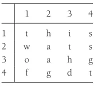
A second problem is to solve a popular word puzzle. The input consists of a two-dimensional array of letters and a list of words. The object is to find the words in the puzzle. These words may be horizontal, vertical, or diagonal in any direction. As an example, the puzzle shown in Figure 1.1 contains the wordsthis, two, fat,andthat.The wordthisbegins at row 1, column 1, or (1,1), and extends to (1,4);twogoes from (1,1) to (3,1);fatgoes from (4,1) to (2,3); andthatgoes from (4,4) to (1,1).
Again, there are at least two straightforward algorithms that solve the problem. For each word in the word list, we check each ordered triple (row, column, orientation) for the pres-ence of the word. This amounts to lots of nestedforloops but is basically straightforward. Alternatively, for each ordered quadruple (row, column, orientation, number of characters) that doesn’t run off an end of the puzzle, we can test whether the word indicated is in the word list. Again, this amounts to lots of nestedforloops. It is possible to save some time if the maximum number of characters in any word is known.
It is relatively easy to code up either method of solution and solve many of the real-life puzzles commonly published in magazines. These typically have 16 rows, 16 columns, and 40 or so words. Suppose, however, we consider the variation where only the puzzle board is given and the word list is essentially an English dictionary. Both of the solutions proposed require considerable time to solve this problem and therefore might not be acceptable. However, it is possible, even with a large word list, to solve the problem very quickly.
An important concept is that, in many problems, writing a working program is not good enough. If the program is to be run on a large data set, then the running time becomes an issue. Throughout this book we will see how to estimate the running time of a program for large inputs and, more important, how to compare the running times of two programs without actually coding them. We will see techniques for drastically improving the speed of a program and for determining program bottlenecks. These techniques will enable us to find the section of the code on which to concentrate our optimization efforts.
1.2 Mathematics Review
1.2.1 Exponents
XAXB=XA+B XA
XB =X A−B
(XA)B=XAB XN+XN=2XN=X2N
2N+2N=2N+1
1.2.2 Logarithms
In computer science, all logarithms are to the base 2 unless specified otherwise.
Definition 1.1
XA=Bif and only if logXB=A
Several convenient equalities follow from this definition.
Theorem 1.1
logAB= logCB
logCA; A,B,C>0,A=1 Proof
Let X = logCB, Y = logCA, and Z = logAB. Then, by the definition of loga-rithms, CX = B, CY = A, and AZ = B. Combining these three equalities yields
B=CX=(CY)Z. Therefore,X=YZ,which impliesZ=X/Y, proving the theorem. Theorem 1.2
logAB=logA+logB; A,B>0 Proof
LetX = logA,Y = logB, and Z = logAB. Then, assuming the default base of 2, 2X = A, 2Y = B, and 2Z = AB. Combining the last three equalities yields 2X2Y =AB=2Z. Therefore,X+Y=Z, which proves the theorem.
Some other useful formulas, which can all be derived in a similar manner, follow.
logA/B=logA−logB log(AB)=BlogA logX<X for allX>0
1.2.3 Series
The easiest formulas to remember are
N
i=0
2i=2N+1−1 and the companion,
N
i=0 Ai=A
N+1−1 A−1 In the latter formula, if 0<A<1, then
N
i=0
Ai≤ 1 1−A
and asN tends to ∞, the sum approaches 1/(1−A). These are the “geometric series” formulas.
We can derive the last formula for∞i=0Ai(0<A<1) in the following manner. Let Sbe the sum. Then
S=1+A+A2+A3+A4+A5+ · · · Then
AS=A+A2+A3+A4+A5+ · · ·
If we subtract these two equations (which is permissible only for a convergent series), virtually all the terms on the right side cancel, leaving
S−AS=1 which implies that
S= 1 1−A
We can use this same technique to compute∞i=1i/2i, a sum that occurs frequently.
We write
S= 1 2+
2 22 +
3 23 +
4 24 +
5 25+ · · · and multiply by 2, obtaining
2S=1+2 2+
3 22 +
4 23 +
5 24 +
6 25 + · · · Subtracting these two equations yields
S=1+1 2+
1 22 +
1 23 +
1 24 +
Another type of common series in analysis is the arithmetic series. Any such series can be evaluated from the basic formula:
N
i=1
i=N(N+1)
2 ≈
N2 2
For instance, to find the sum 2+5+8+ · · · +(3k−1), rewrite it as 3(1+2+3+
· · ·+k)−(1+1+1+· · ·+1), which is clearly 3k(k+1)/2−k. Another way to remember this is to add the first and last terms (total 3k+1), the second and next-to-last terms (total 3k+1), and so on. Since there arek/2 of these pairs, the total sum isk(3k+1)/2, which is the same answer as before.
The next two formulas pop up now and then but are fairly uncommon.
N
i=1
i2=N(N+1)(2N+1)
6 ≈
N3 3
N
i=1 ik≈ N
k+1
|k+1| k= −1
Whenk = −1, the latter formula is not valid. We then need the following formula, which is used far more in computer science than in other mathematical disciplines. The numbersHNare known as the harmonic numbers, and the sum is known as a harmonic
sum. The error in the following approximation tends toγ ≈0.57721566, which is known asEuler’s constant.
HN= N
i=1 1
i ≈logeN These two formulas are just general algebraic manipulations:
N
i=1
f(N)=Nf(N)
N
i=n0 f(i)=
N
i=1 f(i)−
n0−1
i=1 f(i)
1.2.4 Modular Arithmetic
Often,Nis a prime number. In that case, there are three important theorems:
First, if N is prime, then ab ≡ 0 (mod N) is true if and only if a ≡ 0 (mod N) orb ≡ 0 (mod N). In other words, if a prime number N divides a product of two numbers, it divides at least one of the two numbers.
Second, if N is prime, then the equation ax ≡ 1 (mod N) has a unique solution (modN) for all 0<a<N. This solution, 0<x<N, is themultiplicative inverse. Third, if N is prime, then the equation x2 ≡ a (mod N) has either two solutions (modN) for all 0<a<N, or it has no solutions.
There are many theorems that apply to modular arithmetic, and some of them require extraordinary proofs in number theory. We will use modular arithmetic sparingly, and the preceding theorems will suffice.
1.2.5 The
P
Word
The two most common ways of proving statements in data-structure analysis are proof by induction and proof by contradiction (and occasionally proof by intimidation, used by professors only). The best way of proving that a theorem is false is by exhibiting a counterexample.
Proof by Induction
A proof by induction has two standard parts. The first step is proving abase case,that is, establishing that a theorem is true for some small (usually degenerate) value(s); this step is almost always trivial. Next, aninductive hypothesisis assumed. Generally this means that the theorem is assumed to be true for all cases up to some limitk. Using this assumption, the theorem is then shown to be true for the next value, which is typicallyk+1. This proves the theorem (as long askis finite).
As an example, we prove that the Fibonacci numbers,F0=1,F1=1,F2=2,F3=3, F4=5, . . . ,Fi=Fi−1+Fi−2, satisfyFi<(5/3)i, fori≥1. (Some definitions haveF0=0, which shifts the series.) To do this, we first verify that the theorem is true for the trivial cases. It is easy to verify thatF1 =1 <5/3 andF2 =2< 25/9; this proves the basis. We assume that the theorem is true fori=1, 2,. . .,k; this is the inductive hypothesis. To prove the theorem, we need to show thatFk+1<(5/3)k+1. We have
Fk+1=Fk+Fk−1
by the definition, and we can use the inductive hypothesis on the right-hand side, obtaining
Fk+1<(5/3)k+(5/3)k−1
Fk+1<(3/5+9/25)(5/3)k+1 <(24/25)(5/3)k+1 <(5/3)k+1
proving the theorem.
As a second example, we establish the following theorem.
Theorem 1.3
IfN≥1, thenNi=1i2= N(N+1)(26 N+1) Proof
The proof is by induction. For the basis, it is readily seen that the theorem is true when N=1. For the inductive hypothesis, assume that the theorem is true for 1≤k≤N. We will establish that, under this assumption, the theorem is true forN+1. We have
N+1
i=1 i2=
N
i=1
i2+(N+1)2 Applying the inductive hypothesis, we obtain
N+1
i=1
i2= N(N+1)(2N+1)
6 +(N+1)
2
=(N+1)
N(2N+1)
6 +(N+1)
=(N+1)2N
2+7N+6 6
= (N+1)(N+2)(2N+3)
6 Thus,
N+1
i=1
i2= (N+1)[(N+1)+1][2(N+1)+1] 6
proving the theorem.
Proof by Counterexample
The statement Fk ≤ k2 is false. The easiest way to prove this is to compute F11 = 144>112.
Proof by Contradiction
Proof by contradiction proceeds by assuming that the theorem is false and showing that this assumption implies that some known property is false, and hence the original assumption was erroneous. A classic example is the proof that there is an infinite number of primes. To prove this, we assume that the theorem is false, so that there is some largest primePk. Let
N=P1P2P3· · ·Pk+1
Clearly, N is larger than Pk, so, by assumption, N is not prime. However, none of
P1,P2,. . .,PkdividesNexactly, because there will always be a remainder of 1. This is a
con-tradiction, because every number is either prime or a product of primes. Hence, the original assumption, thatPkis the largest prime, is false, which implies that the theorem is true.
1.3 A Brief Introduction to Recursion
Most mathematical functions that we are familiar with are described by a simple formula. For instance, we can convert temperatures from Fahrenheit to Celsius by applying the formula
C=5(F−32)/9
Given this formula, it is trivial to write a C++ function; with declarations and braces removed, the one-line formula translates to one line of C++.
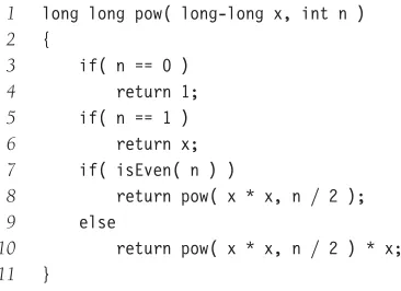
Mathematical functions are sometimes defined in a less standard form. As an example, we can define a function f, valid on nonnegative integers, that satisfies f(0) = 0 and f(x) = 2f(x−1)+x2. From this definition we see thatf(1) =1,f(2) =6,f(3) =21, andf(4)=58. A function that is defined in terms of itself is calledrecursive. C++ allows functions to be recursive.1It is important to remember that what C++ provides is merely an attempt to follow the recursive spirit. Not all mathematically recursive functions are efficiently (or correctly) implemented by C++’s simulation of recursion. The idea is that the recursive functionf ought to be expressible in only a few lines, just like a nonrecursive function. Figure 1.2 shows the recursive implementation off.
Lines 3 and 4 handle what is known as the base case, that is, the value for which the function is directly known without resorting to recursion. Just as declaring f(x) = 2f(x−1)+x2 is meaningless, mathematically, without including the fact that f(0)=0, the recursive C++ function doesn’t make sense without a base case. Line 6 makes the recursive call.
1 int f( int x ) 2 {
3 if( x == 0 )
4 return 0;
5 else
6 return 2 * f( x - 1 ) + x * x;
7 }
Figure 1.2 A recursive function
1Using recursion for numerical calculations is usually a bad idea. We have done so to illustrate the basic
There are several important and possibly confusing points about recursion. A common question is: Isn’t this just circular logic? The answer is that although we are defining a function in terms of itself, we are not defining a particular instance of the function in terms of itself. In other words, evaluatingf(5) by computingf(5) would be circular. Evaluating f(5) by computingf(4) is not circular—unless, of course,f(4) is evaluated by eventually computingf(5). The two most important issues are probably thehowandwhyquestions. In Chapter 3, thehowand whyissues are formally resolved. We will give an incomplete description here.
It turns out that recursive calls are handled no differently from any others. Iffis called with the value of 4, then line 6 requires the computation of 2∗f(3)+4∗4. Thus, a call is made to computef(3). This requires the computation of 2∗f(2)+3∗3. Therefore, another call is made to computef(2). This means that 2∗f(1)+2∗2 must be evaluated. To do so, f(1) is computed as 2∗f(0)+1∗1. Now,f(0) must be evaluated. Since this is a base case, we know a priori thatf(0)=0. This enables the completion of the calculation forf(1), which is now seen to be 1. Thenf(2),f(3), and finallyf(4) can be determined. All the bookkeeping needed to keep track of pending function calls (those started but waiting for a recursive call to complete), along with their variables, is done by the computer automatically. An important point, however, is that recursive calls will keep on being made until a base case is reached. For instance, an attempt to evaluatef(−1) will result in calls tof(−2),f(−3), and so on. Since this will never get to a base case, the program won’t be able to compute the answer (which is undefined anyway). Occasionally, a much more subtle error is made, which is exhibited in Figure 1.3. The error in Figure 1.3 is thatbad(1)is defined, by line 6, to bebad(1). Obviously, this doesn’t give any clue as to whatbad(1) actually is. The computer will thus repeatedly make calls to bad(1) in an attempt to resolve its values. Eventually, its bookkeeping system will run out of space, and the program will terminate abnormally. Generally, we would say that this function doesn’t work for one special case but is correct otherwise. This isn’t true here, sincebad(2)callsbad(1). Thus,bad(2)cannot be evaluated either. Furthermore,bad(3),bad(4), andbad(5)all make calls tobad(2). Since bad(2)is not evaluable, none of these values are either. In fact, this program doesn’t work for any nonnegative value ofn, except 0. With recursive programs, there is no such thing as a “special case.”
These considerations lead to the first two fundamental rules of recursion:
1. Base cases. You must always have some base cases, which can be solved without recursion.
2. Making progress. For the cases that are to be solved recursively, the recursive call must always be to a case that makes progress toward a base case.
1 int bad( int n ) 2 {
3 if( n == 0 )
4 return 0;
5 else
6 return bad( n / 3 + 1 ) + n - 1; 7 }
Throughout this book, we will use recursion to solve problems. As an example of a nonmathematical use, consider a large dictionary. Words in dictionaries are defined in terms of other words. When we look up a word, we might not always understand the definition, so we might have to look up words in the definition. Likewise, we might not understand some of those, so we might have to continue this search for a while. Because the dictionary is finite, eventually either (1) we will come to a point where we understand all of the words in some definition (and thus understand that definition and retrace our path through the other definitions) or (2) we will find that the definitions are circular and we are stuck, or that some word we need to understand for a definition is not in the dictionary. Our recursive strategy to understand words is as follows: If we know the meaning of a word, then we are done; otherwise, we look the word up in the dictionary. If we understand all the words in the definition, we are done; otherwise, we figure out what the definition means byrecursivelylooking up the words we don’t know. This procedure will terminate if the dictionary is well defined but can loop indefinitely if a word is either not defined or circularly defined.
Printing Out Numbers
Suppose we have a positive integer,n, that we wish to print out. Our routine will have the headingprintOut(n). Assume that the only I/O routines available will take a single-digit number and output it. We will call this routineprintDigit; for example,printDigit(4)will output a 4.
Recursion provides a very clean solution to this problem. To print out 76234, we need to first print out 7623 and then print out 4. The second step is easily accomplished with the statementprintDigit(n%10), but the first doesn’t seem any simpler than the original problem. Indeed it is virtually the same problem, so we can solve it recursively with the statementprintOut(n/10).
This tells us how to solve the general problem, but we still need to make sure that the program doesn’t loop indefinitely. Since we haven’t defined a base case yet, it is clear that we still have something to do. Our base case will beprintDigit(n) if 0 ≤ n <10. NowprintOut(n)is defined for every positive number from 0 to 9, and larger numbers are defined in terms of a smaller positive number. Thus, there is no cycle. The entire function is shown in Figure 1.4.
We have made no effort to do this efficiently. We could have avoided using the mod routine (which can be very expensive) because n%10 = n − n/10 ∗10 is true for positiven.2
1 void printOut( int n ) // Print nonnegative n 2 {
3 if( n >= 10 )
4 printOut( n / 10 );
5 printDigit( n % 10 ); 6 }
Figure 1.4 Recursive routine to print an integer
Recursion and Induction
Let us prove (somewhat) rigorously that the recursive number-printing program works. To do so, we’ll use a proof by induction.
Theorem 1.4
The recursive number-printing algorithm is correct forn≥0. Proof(By induction on the number of digits inn)
First, if nhas one digit, then the program is trivially correct, since it merely makes a call toprintDigit. Assume then thatprintOutworks for all numbers ofkor fewer digits. A number ofk+1 digits is expressed by its firstkdigits followed by its least significant digit. But the number formed by the firstkdigits is exactlyn/10, which, by the inductive hypothesis, is correctly printed, and the last digit isn mod 10, so the program prints out any (k+1)-digit number correctly. Thus, by induction, all numbers are correctly printed.
This proof probably seems a little strange in that it is virtually identical to the algorithm description. It illustrates that in designing a recursive program, all smaller instances of the same problem (which are on the path to a base case) may beassumedto work correctly. The recursive program needs only to combine solutions to smaller problems, which are “mag-ically” obtained by recursion, into a solution for the current problem. The mathematical justification for this is proof by induction. This gives the third rule of recursion:
3. Design rule. Assume that all the recursive calls work.
This rule is important because it means that when designing recursive programs, you generally don’t need to know the details of the bookkeeping arrangements, and you don’t have to try to trace through the myriad of recursive calls. Frequently, it is extremely difficult to track down the actual sequence of recursive calls. Of course, in many cases this is an indication of a good use of recursion, since the computer is being allowed to work out the complicated details.
The main problem with recursion is the hidden bookkeeping costs. Although these costs are almost always justifiable, because recursive programs not only simplify the algo-rithm design but also tend to give cleaner code, recursion should not be used as a substitute for a simpleforloop. We’ll discuss the overhead involved in recursion in more detail in Section 3.6.
When writing recursive routines, it is crucial to keep in mind the four basic rules of recursion:
1. Base cases. You must always have some base cases, which can be solved without recursion.
2. Making progress. For the cases that are to be solved recursively, the recursive call must always be to a case that makes progress toward a base case.
3. Design rule. Assume that all the recursive calls work.
The fourth rule, which will be justified (along with its nickname) in later sections, is the reason that it is generally a bad idea to use recursion to evaluate simple mathematical func-tions, such as the Fibonacci numbers. As long as you keep these rules in mind, recursive programming should be straightforward.
1.4 C++ Classes
In this text, we will write many data structures. All of the data structures will be objects that store data (usually a collection of identically typed items) and will provide functions that manipulate the collection. In C++ (and other languages), this is accomplished by using aclass. This section describes the C++ class.
1.4.1 Basic
class
Syntax
A class in C++ consists of itsmembers. These members can be either data or functions. The functions are calledmember functions. Each instance of a class is anobject. Each object contains the data components specified in the class (unless the data components are static, a detail that can be safely ignored for now). A member function is used to act on an object. Often member functions are calledmethods.
As an example, Figure 1.5 is the IntCell class. In the IntCell class, each instance of the IntCell—an IntCell object—contains a single data member named storedValue. Everything else in this particular class is a method. In our example, there are four methods. Two of these methods arereadand write. The other two are special methods known as constructors. Let us describe some key features.
First, notice the two labelspublic and private. These labels determine visibility of class members. In this example, everything except thestoredValuedata member ispublic. storedValueisprivate. A member that ispublicmay be accessed by any method in any class. A member that isprivatemay only be accessed by methods in its class. Typically, data members are declaredprivate, thus restricting access to internal details of the class, while methods intended for general use are madepublic. This is known asinformation hiding. By usingprivatedata members, we can change the internal representation of the object without having an effect on other parts of the program that use the object. This is because the object is accessed through thepublicmember functions, whose viewable behavior remains unchanged. The users of the class do not need to know internal details of how the class is implemented. In many cases, having this access leads to trouble. For instance, in a class that stores dates using month, day, and year, by making the month, day, and yearprivate, we prohibit an outsider from setting these data members to illegal dates, such as Feb 29, 2013. However, some methods may be for internal use and can beprivate. In a class, all members areprivateby default, so the initialpublicis not optional.
1 /**
2 * A class for simulating an integer memory cell. 3 */
4 class IntCell 5 {
6 public:
7 /**
8 * Construct the IntCell. 9 * Initial value is 0.
10 */
11 IntCell( )
12 { storedValue = 0; }
13
14 /**
15 * Construct the IntCell.
16 * Initial value is initialValue.
17 */
18 IntCell( int initialValue ) 19 { storedValue = initialValue; } 20
21 /**
22 * Return the stored value.
23 */
24 int read( )
25 { return storedValue; } 26
27 /**
28 * Change the stored value to x.
29 */
30 void write( int x )
31 { storedValue = x; }
32
33 private:
34 int storedValue; 35 };
Figure 1.5 A complete declaration of anIntCellclass
1.4.2 Extra Constructor Syntax and Accessors
Although the class works as written, there is some extra syntax that makes for better code. Four changes are shown in Figure 1.6 (we omit comments for brevity). The differences are as follows:
Default Parameters
constructor, which is implied because the one-parameter constructor says that initialValue is optional. The default value of 0 signifies that 0 is used if no para-meter is provided. Default parapara-meters can be used in any function, but they are most commonly used in constructors.
Initialization List
TheIntCellconstructor uses aninitialization list(Figure 1.6, line 8) prior to the body of the constructor. The initialization list is used to initialize the data members directly. In Figure 1.6, there’s hardly a difference, but using initialization lists instead of an assignment statement in the body saves time in the case where the data members are class types that have complex initializations. In some cases it is required. For instance, if a data member is const(meaning that it is not changeable after the object has been constructed), then the data member’s value can only be initialized in the initialization list. Also, if a data member is itself a class type that does not have a zero-parameter constructor, then it must be initialized in the initialization list.
Line 8 in Figure 1.6 uses the syntax
: storedValue{ initialValue } { }
instead of the traditional
: storedValue( initialValue ) { }
The use of braces instead of parentheses is new in C++11 and is part of a larger effort to provide a uniform syntax for initialization everywhere. Generally speaking, anywhere you can initialize, you can do so by enclosing initializations in braces (though there is one important exception, in Section 1.4.4, relating to vectors).
1 /**
2 * A class for simulating an integer memory cell. 3 */
4 class IntCell 5 {
6 public:
7 explicit IntCell( int initialValue = 0 ) 8 : storedValue{ initialValue } { } 9 int read( ) const
10 { return storedValue; } 11 void write( int x )
12 { storedValue = x; }
13
14 private:
15 int storedValue; 16 };
explicit
Constructor
The IntCell constructor is explicit. You should make all one-parameter constructors explicit to avoid behind-the-scenes type conversions. Otherwise, there are somewhat lenient rules that will allow type conversions without explicit casting operations. Usually, this is unwanted behavior that destroys strong typing and can lead to hard-to-find bugs. As an example, consider the following:
IntCell obj; // obj is an IntCell
obj = 37; // Should not compile: type mismatch
The code fragment above constructs anIntCell objectobjand then performs an assign-ment stateassign-ment. But the assignassign-ment stateassign-ment should not work, because the right-hand side of the assignment operator is not another IntCell.obj’s writemethod should have been used instead. However, C++ has lenient rules. Normally, a one-parameter constructor defines animplicit type conversion, in which a temporary object is created that makes an assignment (or parameter to a function) compatible. In this case, the compiler would attempt to convert
obj = 37; // Should not compile: type mismatch
into
IntCell temporary = 37; obj = temporary;
Notice that the construction of the temporary can be performed by using the one-parameter constructor. The use ofexplicitmeans that a one-parameter constructor cannot be used to generate an implicit temporary. Thus, sinceIntCell’s constructor is declared explicit, the compiler will correctly complain that there is a type mismatch.
Constant Member Function
A member function that examines but does not change the state of its object is anaccessor. A member function that changes the state is amutator(because it mutates the state of the object). In the typical collection class, for instance,isEmptyis an accessor, whilemakeEmpty is a mutator.
In C++, we can mark each member function as being an accessor or a mutator. Doing so is an important part of the design process and should not be viewed as simply a com-ment. Indeed, there are important semantic consequences. For instance, mutators cannot be applied to constant objects. By default, all member functions are mutators. To make a member function an accessor, we must add the keywordconstafter the closing parenthesis that ends the parameter type list. The const-ness is part of the signature.constcan be used with many different meanings. The function declaration can haveconstin three different contexts. Only theconstafter a closing parenthesis signifies an accessor. Other uses are described in Sections 1.5.3 and 1.5.4.
is marked as an accessor but has an implementation that changes the value of any data member, a compiler error is generated.3
1.4.3 Separation of Interface and Implementation
The class in Figure 1.6 contains all the correct syntactic constructs. However, in C++ it is more common to separate the class interface from its implementation. The interface lists the class and its members (data and functions). The implementation provides implementations of the functions.
Figure 1.7 shows the class interface forIntCell, Figure 1.8 shows the implementation, and Figure 1.9 shows amainroutine that uses theIntCell. Some important points follow.
Preprocessor Commands
The interface is typically placed in a file that ends with .h. Source code that requires knowledge of the interface must#includethe interface file. In our case, this is both the implementation file and the file that containsmain. Occasionally, a complicated project will have files including other files, and there is the danger that an interface might be read twice in the course of compiling a file. This can be illegal. To guard against this, each header file uses the preprocessor to define a symbol when the class interface is read. This is shown on the first two lines in Figure 1.7. The symbol name,IntCell_H, should not appear in any other file; usually, we construct it from the filename. The first line of the interface file
1 #ifndef IntCell_H 2 #define IntCell_H 3
4 /**
5 * A class for simulating an integer memory cell. 6 */
7 class IntCell 8 {
9 public:
10 explicit IntCell( int initialValue = 0 ); 11 int read( ) const;
12 void write( int x ); 13
14 private:
15 int storedValue; 16 };
17
18 #endif
Figure 1.7 IntCellclass interface in fileIntCell.h
1 #include "IntCell.h" 2
3 /**
4 * Construct the IntCell with initialValue 5 */
6 IntCell::IntCell( int initialValue ) : storedValue{ initialValue } 7 {
8 } 9 10 /**
11 * Return the stored value. 12 */
13 int IntCell::read( ) const 14 {
15 return storedValue; 16 }
17 18 /** 19 * Store x. 20 */
21 void IntCell::write( int x ) 22 {
23 storedValue = x; 24 }
Figure 1.8 IntCellclass implementation in fileIntCell.cpp
1 #include <iostream> 2 #include "IntCell.h" 3 using namespace std; 4
5 int main( ) 6 {
7 IntCell m;
8
9 m.write( 5 );
10 cout << "Cell contents: " << m.read( ) << endl; 11
12 return 0;
13 }
tests whether the symbol is undefined. If so, we can process the file. Otherwise, we do not process the file (by skipping to the#endif), because we know that we have already read the file.
Scope Resolution Operator
In the implementation file, which typically ends in.cpp,.cc, or.C, each member function must identify the class that it is part of. Otherwise, it would be assumed that the function is in global scope (and zillions of errors would result). The syntax isClassName::member. The::is called thescope resolution operator.
Signatures Must Match Exactly
The signature of an implemented member function must match exactly the signature listed in the class interface. Recall that whether a member function is an accessor (via theconst at the end) or a mutator is part of the signature. Thus an error would result if, for example, the constwas omitted from exactly one of the read signatures in Figures 1.7 and 1.8. Note that default parameters are specified in the interface only. They are omitted in the implementation.
Objects Are Declared Like Primitive Types
In classic C++, an object is declared just like a primitive type. Thus the following are legal declarations of anIntCellobject:
IntCell obj1; // Zero parameter constructor IntCell obj2( 12 ); // One parameter constructor
On the other hand, the following are incorrect:
IntCell obj3 = 37; // Constructor is explicit IntCell obj4( ); // Function declaration
The declaration ofobj3is illegal because the one-parameter constructor isexplicit. It would be legal otherwise. (In other words, in classic C++ a declaration that uses the one-parameter constructor must use the parentheses to signify the initial value.) The declaration forobj4states that it is a function (defined elsewhere) that takes no parameters and returns anIntCell.
The confusion ofobj4is one reason for the uniform initialization syntax using braces. It was ugly that initializing with zero parameter in a constructor initialization list (Fig. 1.6, line 8) would require parentheses with no parameter, but the same syntax would be illegal elsewhere (forobj4). In C++11, we can instead write:
IntCell obj1; // Zero parameter constructor, same as before IntCell obj2{ 12 }; // One parameter constructor, same as before IntCell obj4{ }; // Zero parameter constructor
1 #include <iostream> 2 #include <vector> 3 using namespace std; 4
5 int main( ) 6 {
7 vector<int> squares( 100 ); 8
9 for( int i = 0; i < squares.size( ); ++i )
10 squares[ i ] = i * i;
11
12 for( int i = 0; i < squares.size( ); ++i ) 13 cout << i << " " << squares[ i ] << endl; 14
15 return 0;
16 }
Figure 1.10 Using thevectorclass: stores 100 squares and outputs them
1.4.4
vector
and
string
The C++ standard defines two classes: thevectorandstring.vectoris intended to replace the built-in C++ array, which causes no end of trouble. The problem with the built-in C++ array is that it does not behave like a first-class object. For instance, built-in arrays cannot be copied with=, a built-in array does not remember how many items it can store, and its indexing operator does not check that the index is valid. The built-in string is simply an array of characters, and thus has the liabilities of arrays plus a few more. For instance,== does not correctly compare two built-in strings.
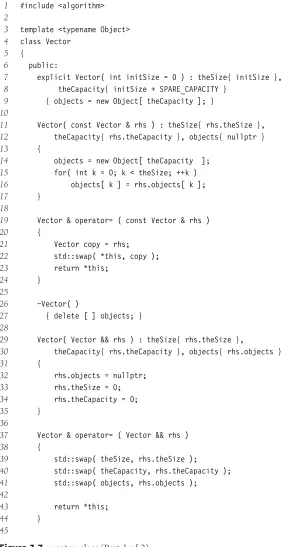
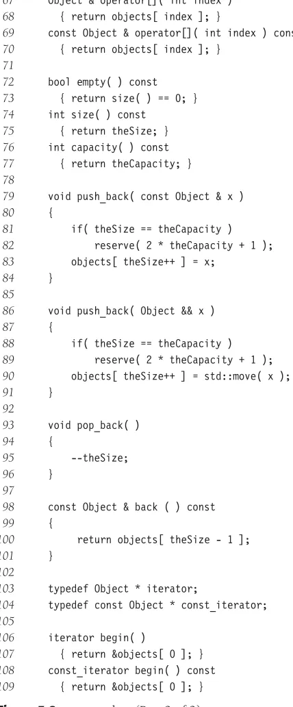
Thevectorandstringclasses in the STL treat arrays and strings as first-class objects. Avector knows how large it is. Twostringobjects can be compared with==,<, and so on. Bothvectorandstringcan be copied with=. If possible, you should avoid using the built-in C++ array and string. We discuss the built-in array in Chapter 3 in the context of showing howvectorcan be implemented.
vectorandstringare easy to use. The code in Figure 1.10 creates avectorthat stores one hundred perfect squares and outputs them. Notice also that size is a method that returns the size of thevector. A nice feature of thevectorthat we explore in Chapter 3 is that it is easy to change its size. In many cases, the initial size is 0 and thevectorgrows as needed.
C++ has long allowed initialization of built-in C++ arrays:
int daysInMonth[ ] = { 31, 28, 31, 30, 31, 30, 31, 31, 30, 31, 30, 31 };
vector<int> daysInMonth( 12 ); // No {} before C++11
daysInMonth[ 0 ] = 31; daysInMonth[ 1 ] = 28; daysInMonth[ 2 ] = 31; daysInMonth[ 3 ] = 30; daysInMonth[ 4 ] = 31; daysInMonth[ 5 ] = 30; daysInMonth[ 6 ] = 31; daysInMonth[ 7 ] = 31; daysInMonth[ 8 ] = 30; daysInMonth[ 9 ] = 31; daysInMonth[ 10 ] = 30; daysInMonth[ 11 ] = 31;
Certainly this leaves something to be desired. C++11 fixes this problem and allows:
vector<int> daysInMonth = { 31, 28, 31, 30, 31, 30, 31, 31, 30, 31, 30, 31 };
Requiring the=in the initialization violates the spirit of uniform initialization, since now we would have to remember when it would be appropriate to use=. Consequently, C++11 also allows (and some prefer):
vector<int> daysInMonth { 31, 28, 31, 30, 31, 30, 31, 31, 30, 31, 30, 31 };
With syntax, however, comes ambiguity, as one sees with the declaration
vector<int> daysInMonth { 12 };
Is this avector of size 12, or is it a vector of size 1 with a single element 12 in position 0? C++11 gives precedence to the initializer list, so in fact this is avector of size 1 with a single element 12 in position 0, and if the intention is to initialize avector of size 12, the old C++ syntax using parentheses must be used:
vector<int> daysInMonth( 12 ); // Must use () to call constructor that takes size
stringis also easy to use and has all the relational and equality operators to compare the states of two strings. Thusstr1==str2istrueif the value of the strings are the same. It also has alengthmethod that returns the string length.
As Figure 1.10 shows, the basic operation on arrays is indexing with []. Thus, the sum of the squares can be computed as:
int sum = 0;
for( int i = 0; i < squares.size( ); ++i ) sum += squares[ i ];
The pattern of accessing every element sequentially in a collection such as an array or a vectoris fundamental, and using array indexing for this purpose does not clearly express the idiom. C++11 adds arangeforsyntax for this purpose. The above fragment can be written instead as:
int sum = 0;
for( int x : squares ) sum += x;
In many cases, the declaration of the type in the range for statement is unneeded; ifsquares is avector<int>, it is obvious thatxis intended to be anint. Thus C++11 also allows the use of the reserved word auto to signify that the compiler will automatically infer the appropriate type:
int sum = 0;
The rangeforloop is appropriate only if every item is being accessed sequentially and only if the index is not needed. Thus, in Figure 1.10 the two loops cannot be rewritten as range forloops, because the indexiis also being used for other purposes. The rangeforloop as shown so far allows only the viewing of items; changing the items can be done using syntax described in Section 1.5.4.
1.5 C++ Details
Like any language, C++ has its share of details and language features. Some of these are discussed in this section.
1.5.1 Pointers
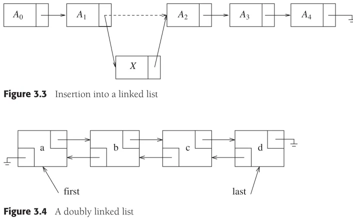
Apointer variableis a variable that stores the address where another object resides. It is the fundamental mechanism used in many data structures. For instance, to store a list of items, we could use a contiguous array, but insertion into the middle of the contiguous array requires relocation of many items. Rather than store the collection in an array, it is common to store each item in a separate, noncontiguous piece of memory, which is allocated as the program runs. Along with each object is a link to the next object. This link is a pointer variable, because it stores a memory location of another object. This is the classic linked list that is discussed in more detail in Chapter 3.
To illustrate the operations that apply to pointers, we rewrite Figure 1.9 to dynamically allocate the IntCell. It must be emphasized that for a simple IntCell class, there is no good reason to write the C++ code this way. We do it only to illustrate dynamic memory allocation in a simple context. Later in the text, we will see more complicated classes, where this technique is useful and necessary. The new version is shown in Figure 1.11.
Declaration
Line 3 illustrates the declaration ofm. The*indicates thatmis a pointer variable; it is allowed to point at anIntCellobject. Thevalueofmis the address of the object that it points at.
1 int main( ) 2 {
3 IntCell *m;
4
5 m = new IntCell{ 0 }; 6 m->write( 5 );
7 cout << "Cell contents: " << m->read( ) << endl; 8
9 delete m;
10 return 0;
11 }
m is uninitialized at this point. In C++, no such check is performed to verify that m is assigned a value prior to being used (however, several vendors make products that do additional checks, including this one). The use of uninitialized pointers typically crashes programs, because they result in access of memory locations that do not exist. In general, it is a good idea to provide an initial value, either by combining lines 3 and 5, or by initializingmto thenullptrpointer.
Dynamic Object Creation
Line 5 illustrates how objects can be created dynamically. In C++ newreturns a pointer to the newly created object. In C++ there are several ways to create an object using its zero-parameter constructor. The following would be legal:
m = new IntCell( ); // OK m = new IntCell{ }; // C++11
m = new IntCell; // Preferred in this text
We generally use the last form because of the problem illustrated byobj4in Section 1.4.3.
Garbage Collection and
delete
In some languages, when an object is no longer referenced, it is subject to automatic garbage collection; the programmer does not have to worry about it. C++ does not have garbage collection. When an object that is allocated by new is no longer referenced, the deleteoperation must be applied to the object (through a pointer). Otherwise, the mem-ory that it consumes is lost (until the program terminates). This is known as amemory leak. Memory leaks are, unfortunately, common occurrences in many C++ programs. Fortunately, many sources of memory leaks can be automatically removed with care. One important rule is to not usenewwhen anautomatic variablecan be used instead. In the original program, theIntCellis not allocated bynewbut instead is allocated as a local vari-able. In that case, the memory for theIntCellis automatically reclaimed when the function in which it is declared returns. Thedeleteoperator is illustrated at line 9 of Figure 1.11.
Assignment and Comparison of Pointers
Assignment and comparison of pointer variables in C++ is based on the value of the pointer, meaning the memory address that it stores. Thus two pointer variables are equal if they point at the same object. If they point at different objects, the pointer variables are not equal, even if the objects being pointed at are themselves equal. Iflhsandrhsare pointer variables (of compatible types), thenlhs=rhsmakeslhspoint at the same object thatrhs points at.4
Accessing Members of an Object through a Pointer
If a pointer variable points at a class type, then a (visible) member of the object being pointed at can be accessed via the -> operator. This is illustrated at lines 6 and 7 of Figure 1.11.