A Tutorial on Graph-Based SLAM

A Tutorial on Graph-Based SLAM

Giorgio Grisetti

Rainer K¨ummerle

Cyrill Stachniss

Wolfram Burgard

Abstract—Being able to build a map of the environment and to simultaneously localize within this map is an essential skill for mobile robots navigating in unknown environments in absence of external referencing systems such as GPS. This so-called simultaneous localization and mapping (SLAM) problem has been one of the most popular research topics in mobile robotics for the last two decades and efficient approaches for solving this task have been proposed. One intuitive way of formulating SLAM is to use a graph whose nodes correspond to the poses of the robot at different points in time and whose edges represent constraints between the poses. The latter are obtained from observations of the environment or from movement actions carried out by the robot. Once such a graph is constructed, the map can be computed by finding the spatial configuration of the nodes that is mostly consistent with the measurements modeled by the edges. In this paper, we provide an introductory description to the graph-based SLAM problem. Furthermore, we discuss a state-of-the-art solution that is based on least-squares error minimization and exploits the structure of the SLAM problems during optimization. The goal of this tutorial is to enable the reader to implement the proposed methods from scratch.

I. INTRODUCTION

To efficiently solve many tasks envisioned to be carried out by mobile robots including transportation, search and rescue, or automated vacuum cleaning robots need a map of the environment. The availability of an accurate map allows for the design of systems that can operate in complex environments only based on their on-board sensors and without relying on external reference system like, e.g., GPS. The acquisition of maps of indoor environments, where typically no GPS is available, has been a major research focus in the robotics community over the last decades. Learning maps under pose uncertainty is often referred to as the simultaneous localization and mapping (SLAM) problem. In the literature, a large variety of solutions to this problem is available. These approaches can be classified either as filtering or smoothing. Filtering approaches model the problem as an on-line state estimation where the state of the system consists in the current robot po-sition and the map. The estimate is augmented and refined by incorporating the new measurements as they become available. Popular techniques like Kalman and information filters [28], [3], particle filters [22], [12], [9], or information filters [7], [31] fall into this category. To highlight their incremental nature, the filtering approaches are usually referred to as on-line SLAM methods. Conversely, smoothing approaches estimate the full trajectory of the robot from the full set of measurements [21], [5], [27]. These approaches address the so-called full SLAM problem, and they typically rely on least-square error minimization techniques.

Figure 1 shows three examples of real robotic systems that use SLAM technology: an autonomous car, a tour-guide robot, and an industrial mobile manipulation robot. Image

(a) shows the autonomous car Junior as well as a model of a parking garage that has been mapped with that car. Thanks to the acquired model, the car is able to park itself autonomously at user selected locations in the garage. Image (b) shows the TPR-Robina robot developed by Toyota which is also used in the context of guided tours in museums. This robot uses SLAM technology to update its map whenever the environment has been changed. Robot manufacturers such as KUKA, recently presented mobile manipulators as shown in Image (c). Here, SLAM technology is needed to operate such devices in flexible way in changing industrial environments. Figure 2 illustrates 2D and 3D maps that can be estimated by the SLAM algorithm discussed in this paper.

An intuitive way to address the SLAM problem is via its so-called graph-based formulation. Solving a graph-based SLAM problem involves to construct a graph whose nodes represent robot poses or landmarks and in which an edge between two nodes encodes a sensor measurement that con-strains the connected poses. Obviously, such constraints can be contradictory since observations are always affected by noise. Once such a graph is constructed, the crucial problem is to find a configuration of the nodes that is maximally consistent with the measurements. This involves solving a large error minimization problem.

The graph-based formulation of the SLAM problem has been proposed by Lu and Milios in 1997 [21]. However, it took several years to make this formulation popular due to the comparably high complexity of solving the error minimization problem using standard techniques. Recent insights into the structure of the SLAM problem and advancements in the fields of sparse linear algebra resulted in efficient approaches to the optimization problem at hand. Consequently, graph-based SLAM methods have undergone a renaissance and currently belong to the state-of-the-art techniques with respect to speed and accuracy. The aim of this tutorial is to introduce the SLAM problem in its probabilistic form and to guide the reader to the synthesis of an effective and state-of-the-art graph-based SLAM method. To understand this tutorial a good knowledge of linear algebra, multivariate minimization, and probability theory are required.

II. PROBABILISTICFORMULATION OFSLAM

(a) (b) (c)

Fig. 1. Applications of SLAM technology. (a) An autonomous instrumented car developed at Stanford. This car can acquire maps by utilizing only its on-board sensors. These maps can be subsequently used for autonomous navigation. (b) The museum guide robot TPR-Robina developed by Toyota (picture courtesy of Toyota Motor Company). This robot acquires a new map every time the museum is reconfigured. (c) The KUKA Concept robot “Omnirob”, a mobile manipulator designed autonomously navigate and operate in the environment with the sole use of its on-board sensors (picture courtesy of KUKA Roboter GmbH).

and perceptions of the environment z1:T = {z1, . . . ,zT}. Solving the full SLAM problem consists of estimating the posterior probability of the robot’s trajectory x1:T and the map m of the environment given all the measurements plus an initial positionx0:

p(x1:T,m|z1:T,u1:T,x0). (1)

The initial position x0 defines the position of the map and can be chosen arbitrarily. For convenience of notation, in the remainder of this document we will omitx0. The poses x1:T and the odometry u1:T are usually represented as 2D or 3D transformations inSE(2)or inSE(3), while the map can be represented in different ways. Maps can be parametrized as a set of spatially located landmarks, by dense representations like occupancy grids, surface maps, or by raw sensor measure-ments. The choice of a particular map representation depends on the sensors used, on the characteristics of the environment, and on the estimation algorithm. Landmark maps [28], [22] are often preferred in environments where locally distinguishable features can be identified and especially when cameras are used. In contrast, dense representations [33], [12], [9] are usually used in conjunction with range sensors. Independently of the type of the representation, the map is defined by the measurements and the locations where these measurements have been acquired [17], [18]. Figure 2 illustrates three typical dense map representations for 3D and 2D: multilevel surface maps, point clouds and occupancy grids. Figure 3 shows a typical 2D landmark based map.

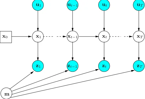
Estimating the posterior given in (1) involves operating in high dimensional state spaces. This would not be tractable if the SLAM problem would not have a well defined structure. This structure arises from certain and commonly done assump-tions, namely the static world assumption and the Markov assumption. A convenient way to describe this structure is via the dynamic Bayesian network (DBN) depicted in Figure 4. A Bayesian network is a graphical model that describes a stochastic process as a directed graph. The graph has one node for each random variable in the process, and a directed edge (or arrow) between two nodes models a conditional dependence between them.

-20 -10 0 10 20 30

-50 -40 -30 -20 -10 0 10 20 landmarks

trajectory

Fig. 3. Landmark based maps acquired at the German Aerospace Center. In this setup the landmarks consist in white circles painted on the ground that are detected by the robot through vision, as shown in the left image. The right image illustrates the trajectory of the robot and the estimated positions of the landmarks. These images are courtesy of Udo Frese and Christoph Hertzberg.

x0 x1 xt−1 xt xT

u1 ut−1 ut uT

z1 z_t−1 zt zT

m

Fig. 4. Dynamic Bayesian Network of the SLAM process.

(a) (b) (c)

Fig. 2. (a) A 3D map of the Stanford parking garage acquired with an instrumented car (bottom), and the corresponding satellite view (top). This map has been subsequently used to realize an autonomous parking behavior. (b) Point cloud map acquired at the university of Freiburg (courtesy of Kai. M. Wurm) and relative satellite image. (c) Occupancy grid map acquired at the hospital of Freiburg. Top: a bird’s eye view of the area, bottom: the occupancy grid representation. The gray areas represent unobserved regions, the white part represents traversable space while the black points indicate occupied regions.

represented by the two edges leading toxtand represents the probability that the robot at timet is inx_tgiven that at time

t−1 it was in x_tand it acquired an odometry measurement

u_t.

The observation modelp(zt|xt,mt)models the probabil-ity of performing the observationztgiven that the robot is at locationxtin the map. It is represented by the arrows entering in zt. The exteroceptive observation zt depends only on the current location xt of the robot and on the (static) map m. Expressing SLAM as a DBN highlights its temporal structure, and therefore this formalism is well suited to describe filtering processes that can be used to tackle the SLAM problem.

An alternative representation to the DBN is via the so-called “graph-based” or “network-based” formulation of the SLAM problem, that highlights the underlying spatial structure. In graph-based SLAM, the poses of the robot are modeled by nodes in a graph and labeled with their position in the environment [21], [18]. Spatial constraints between poses that result from observations zt or from odometry measurements

ut are encoded in the edges between the nodes. More in detail, a graph-based SLAM algorithm constructs a graph out of the raw sensor measurements. Each node in the graph represents a robot position and a measurement acquired at that position. An edge between two nodes represents a spatial constraint relating the two robot poses. A constraint consists in a probability distribution over the relative transformations between the two poses. These transformations are either odom-etry measurements between sequential robot positions or are determined by aligning the observations acquired at the two robot locations. Once the graph is constructed one seeks to find the configuration of the robot poses that best satisfies the constraints. Thus, in graph-based SLAM the problem is decoupled in two tasks: constructing the graph from the raw measurements (graph construction), determining the most likely configuration of the poses given the edges of the graph (graph optimization). The graph construction is usually called front-end and it is heavily sensor dependent, while the second part is called back-end and relies on an abstract representation

Fig. 5. Pose-graph corresponding to a data-set recorded at MIT Killian Court (courtesy of Mike Bosse and John Leonard) (left) and after (right) optimization. The maps are obtained by rendering the laser scans according to the robot positions in the graph.

of the data which is sensor agnostic. A short example of a front-end for 2D laser SLAM is described in Section V-A. In this tutorial we will describe an easy-to-implement but efficient back-end for graph-based SLAM. Figure 5 depicts an uncorrected pose-graph and the corresponding corrected one.

III. RELATEDWORK

There is a large variety of SLAM approaches available in the robotics community. Throughout this tutorial we focus on graph-based approaches and therefore will consider such ap-proaches in the discussion of related work. Lu and Milios [21] were the first to refine a map by globally optimizing the system of equations to reduce the error introduced by constraints. Gutmann and Konolige [11] proposed an effective way for constructing such a network and for detecting loop closures while running an incremental estimation algorithm. Since then, many approaches for minimizing the error in the constraint network have been proposed. For example, Howard et al. [15] apply relaxation to localize the robot and build a map. Frese

et al. [8] propose a variant of Gauss-Seidel relaxation called

resolutions. Dellaert and Kaess [5] were the first to exploit sparse matrix factorizations to solve the linearized problem in off-line SLAM. Subsequently Kaess et al. [16] presented iSAM, an on-line version that exploits partial reorderings to compute the sparse factorization.

Recently, Konolige et al. [19] proposed an open-source implementation of a pose-graph method that constructs the linearized system in an efficient way. Olson et al. [27] pre-sented an efficient optimization approach which is based on the stochastic gradient descent and can efficiently correct even large pose-graphs. Grisetti et al. proposed an extension of Olson’s approach that uses a tree parametrization of the nodes in 2D and 3D. In this way, they increase the convergence speed [10].

GraphSLAM [32] applies variable elimination techniques to reduce the dimensionality of the optimization problem. The ATLAS framework [2] constructs a two-level hierarchy of graphs and employs a Kalman filter to construct the bottom level. Then, a global optimization approach aligns the local maps at the second level. Similar to ATLAS, Estrada et al. proposed Hierarchical SLAM [6] as a technique for using independent local maps.

Most optimization techniques focus on computing the best map given the constraints and are called SLAM back-ends. In contrast to that, SLAM front-ends seek to interpret the sensor data to obtain the constraints that are the basis for the optimization approaches. Olson [25], for example, pre-sented a front-end with outlier rejection based on spectral clustering. For making data associations in the SLAM front-ends statistical tests such as theχ2 test or joint compatibility test [23] are often applied. The work of N¨uchter et al. [24] aims at building an integrated SLAM system for 3D mapping. The main focus lies on the SLAM front-end for finding constraints. For optimization, a variant of the approach of Lu and Milios [21] for 3D settings is applied. The methods proposed in this paper can be effectively applied to all these front-ends.

IV. GRAPH-BASEDSLAM

A graph-based SLAM approach constructs a simplified esti-mation problem by abstracting the raw sensor measurements. These raw measurements are replaced by the edges in the graph which can then be seen as “virtual measurements”. More in detail an edge between two nodes is labeled with a probability distribution over the relative locations of the two poses, conditioned to their mutual measurements. In general, the observation model p(zt | xt,mt) is multi-modal and therefore the Gaussian assumption does not hold. This means that a single observationztmight result in multiple potential edges connecting different poses in the graph and the graph connectivity needs itself to be described as a probability distribution. Directly dealing with this multi-modality in the estimation process would lead to a combinatorial explosion of the complexity. As a result of that, most practical approaches restrict the estimate to the most likely topology. Thus, one needs to determine the most likely constraint resulting from an observation. This decision depends on the probability

x1

x2 x3

x_i x_j

x_t−1 x_t

x_T

heij,Ω_iji

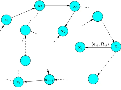
Fig. 6. A pose-graph representation of a SLAM process. Every node in the graph corresponds to a robot pose. Nearby poses are connected by edges that model spatial constraints between robot poses arising from measurements. Edges e_t−1t between consecutive poses model odometry measurements,

while the other edges represent spatial constraints arising from multiple observations of the same part of the environment.

distribution over the robot poses. This problem is known as data association and is usually addressed by the SLAM front-end. To compute the correct data-association, a front-end usually requires a consistent estimate of the conditional prior over the robot trajectory p(x1:T | z1:T,u1:T). This requires to interleave the execution of the front-end and of the back-end while the robot explores the environment. Therefore, the accuracy and the efficiency of the back-end is crucial to the design of a good SLAM system. In this tutorial, we will not describe sophisticated approaches to the data association problem. Such methods tackle association by means of spectral clustering [27], joint compatibility branch and bound [23], or backtracking [13]. We rather assume that the given front-end provides consistent estimates.

If the observations are affected by (locally) Gaussian noise and the data association is known, the goal of a graph-based mapping algorithm is to compute a Gaussian approximation of the posterior over the robot trajectory. This involves computing the mean of this Gaussian as the configuration of the nodes that maximizes the likelihood of the observations. Once this mean is known the information matrix of the Gaussian can be obtained in a straightforward fashion, as explained in Section IV-B. In the following we will characterize the task of finding this maximum as a constraint optimization problem. We will also introduce parts of the notation illustrated in Figure 6.

Let x= (x1, . . . ,xT)T be a vector of parameters, where

xidescribes the pose of nodei. LetzijandΩijbe respectively the mean and the information matrix of a virtual measurement between the nodeiand the nodej. This virtual measurement is a transformation that makes the observations acquired from

imaximally overlap with the observation acquired fromj. Let

ˆ

log-x_i

x_j z_ij

ˆ

z_ij

Ω_ij

e_ij(xi,x_j)

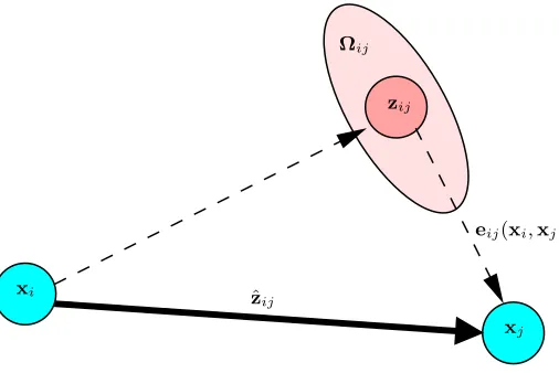
Fig. 7. Aspects of an edge connecting the vertex x_{i and the vertex}x_j. This edge originates from the measurementz_{ij. From the relative position} of the two nodes, it is possible to compute the expected measurementˆz_ij that representsx_{jseen in the frame of}x_{i. The error}e_ij(x_i

,xj)depends on

the displacement between the expected and the real measurement. An edge is fully characterized by its error functione_ij(x_i

,xj)and by the information

matrixΩ_{ijof the measurement that accounts for its uncertainty.}

likelihood lij of a measurement zij is therefore

lij ∝[zij−ˆzij(xi,xj)]TΩij[zij−ˆzij(xi,xj)]. (2)

Lete(x_i,x_j,z_ij)be a function that computes a difference between the expected observationzˆij and the real observation

zij gathered by the robot. For simplicity of notation, we will encode the indices of the measurement in the indices of the error function

eij(xi,xj) = zij−ˆzij(xi,xj). (3)

Figure 7 illustrates the functions and the quantities that play a role in defining an edge of the graph. Let C be the set of pairs of indices for which a constraint (observation)zexists. The goal of a maximum likelihood approach is to find the configuration of the nodesx∗that minimizes the negative log likelihood F(x)of all the observations

F(x) = X

hi,ji∈C

eT_ijΩ_ije_ij | {z }

F_ij

, (4)

thus, it seeks to solve the following equation:

x∗ = argmin x

F(x). (5)

In the remainder of this section we will describe an approach to solve Eq. 5 and to compute a Gaussian approximation of the posterior over the robot trajectory. Whereas the pro-posed approach utilizes standard optimization methods, like the Gauss-Newton or the Levenberg-Marquardt algorithms, it is particularly efficient because it effectively exploits the structure of the problem.

We first describe a direct implementation of traditional non-linear least-squares optimization. Subsequently, we introduce a workaround that allows to deal with the singularities in the representation of the robot poses in an elegant manner.

A. Error Minimization via Iterative Local Linearizations

If a good initial guessx˘ of the robot’s poses is known, the numerical solution of Eq. (5) can be obtained by using the popular Gauss-Newton or Levenberg-Marquardt algorithms. The idea is to approximate the error function by its first order Taylor expansion around the current initial guessx˘

e_ij(˘x_i+∆x_i,x˘_j+∆x_j) = e_ij(˘x+∆x) (6)

≃ eij+Jij∆x. (7)

Here,Jij is the Jacobian ofeij(x)computed inx˘ andeij

def. = e_ij(˘x). Substituting Eq. (7) in the error termsF_ij of Eq. (4), we obtain:

F_ij(˘x+∆x)

= eij(˘x+∆x)TΩijeij(˘x+∆x) (8)

≃ (e_ij+J_ij∆x)T_Ω

ij(eij+Jij∆x) (9)

= eT_ijΩ_ije_ij

| {z }

c_ij

+2eT_ijΩ_ijJ_ij

| {z } b_ij

∆x₊∆xTJT_ijΩ_ijJ_ij

| {z } H_ij

∆x₍₁₀₎

= cij+ 2bij∆x+∆xTHij∆x (11)

With this local approximation, we can rewrite the function

F(x)in Eq. (4) as

F(˘x+∆x) = X

hi,ji∈C

F_ij(˘x+∆x) (12)

≃ X

hi,ji∈C

cij+ 2bij∆x+∆xTHij∆x (13)

= c + 2bT∆x+∆xTH∆x. (14)

The quadratic form in Eq. (14) is obtained from Eq. (13) by setting c = Pcij, b =Pbij, andH =PHij. It can be minimized in∆x by solving the linear system

H ∆x∗ = −b. (15)

The matrix H is the information matrix of the system, since it is obtained by projecting the measurement error in the space of the trajectories via the Jacobians. It is sparse by construction, having non-zeros between poses connected by a constraint. Its number of non-zero blocks is twice the number of constrains plus the number of nodes. This allows to solve Eq. (15) by sparse Cholesky factorization. An efficient yet compact implementation of sparse Cholesky factorization can be found in the library CSparse [4].

The linearized solution is then obtained by adding to the initial guess the computed increments

x∗ = ˘x+∆x∗. (16)

The popular Gauss-Newton algorithm iterates the linearization in Eq. (14), the solution in Eq. (15), and the update step in Eq. (16). In every iteration, the previous solution is used as the linearization point and the initial guess.

B. Considerations about the Structure of the Linearized Sys-tem

According to Eq. (14), the matrix H and the vector bare obtained by summing up a set of matrices and vectors, one for every constraint. Every constraint will contribute to the system with an addend term. The structure of this addend depends on the Jacobian of the error function. Since the error function of a constraint depends only on the values of two nodes, the Jacobian in Eq. (7) has the following form:

Jij =





0· · ·0 Aij

|{z} nodei

0· · ·0 Bij

|{z} nodej

0· · ·0 

 . (17)

HereAijandBijare the derivatives of the error function with respect to xi andxj. From Eq. (10) we obtain the following structure for the block matrixHij:

H_ij =          . ..

AT_ijΩijAij · · · ATijΩijBij ..

. . .. ...

BT

ijΩijAij · · · BTijΩijBij . ..          (18)

b_ij =          .. .

AT_ijΩijeij .. .

BT ijΩijeij

.. .          (19)

For simplicity of notation we omitted the zero blocks. Algorithm 1 summarizes an iterative Gauss-Newton proce-dure to determine both the mean and the information matrix of the posterior over the robot poses. Since most of the structures in the system are sparse, we recommend to use memory efficient representations to store the Hessian H of the system. Since the structure of the Hessian is known in advance from the connectivity of the graph, we recommend to pre-allocate the Hessian once at the beginning of the iterations and to update it in place by looping over all edges whenever a new linearization is required. Each edge contributes to the blocks H_[ii], H_[ij], H_[ji], and H_[jj] and to the blocks b_[i]

andb_[j] of the coefficient vector. An additional optimization is to compute only the upper triangular part of H, since it is symmetric. Note that the error of a constraint eij depends only on the relative position of the connected poses xi and

xj. Accordingly, the error F(x)of a particular configuration of the posesx is invariant under a rigid transformation of all the poses. This results in Eq. 15 being under determined. To numerically solve this system it is therefore common practice to constrain one of the increments∆xkto be zero. This can be done by adding the identity matrix to the kth diagonal block

H[kk]. Without loss of generality in Algorithm 1 we fix the first node x1. An alternative way to fix a particular node of the pose-graph consists in suppressing thekth _{block row and}

thekth _{block column of the linear system in Eq. 15.}

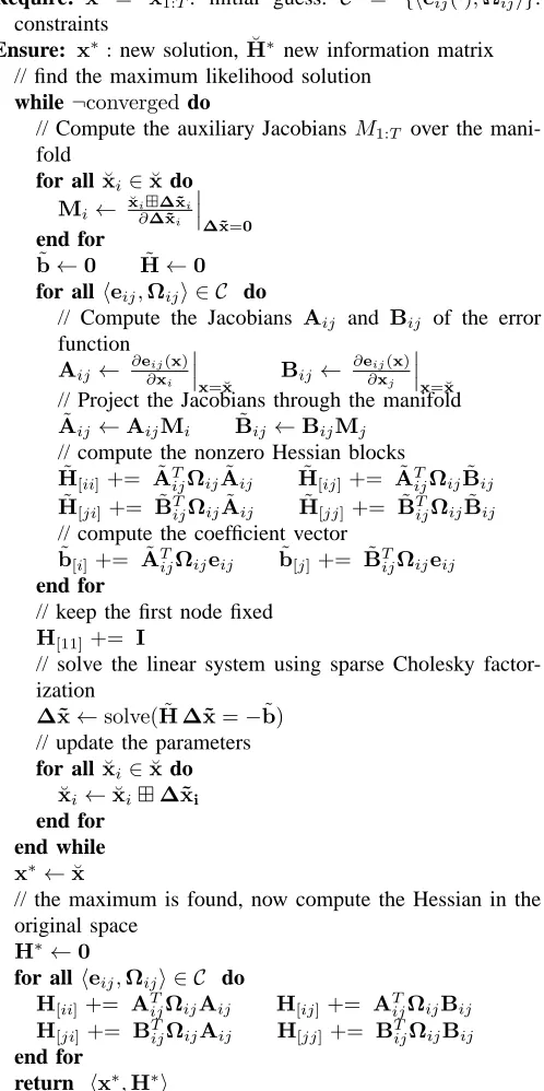
Algorithm 1 Computes the mean x∗ and the information matrix H∗ of the multivariate Gaussian approximation of the robot pose posterior from a graph of constraints.

Require: x˘ = ˘x1:T: initial guess. C = {heij(·),Ωiji}: constraints

Ensure: x∗: new solution,H∗ new information matrix // find the maximum likelihood solution

while ¬convergeddo

b←0 H←0

for all he_ij,Ω_iji ∈ C do

// Compute the Jacobians A_ij and B_ij of the error function

Aij ← ∂

e_ij(x)

∂x_{i x}

=˘x

Bij ← ∂

e_ij(x)

∂x_{j x}

=˘x

// compute the contribution of this constraint to the linear system

H[ii]+= ATijΩijAij H[ij]+= ATijΩijBij

H[ji]+= BTijΩijAij H[jj]+= BTijΩijBij // compute the coefficient vector

b[i] += ATijΩijeij b[j] += BTijΩijeij end for

// keep the first node fixed

H[11]+= I

// solve the linear system using sparse Cholesky factor-ization

∆x←solve(H ∆x=−b)

// update the parameters

˘

x+= ∆x

end while

x∗_←˘x H∗←H

// release the first node

H∗_[11]−= I

return hx∗,H∗i

C. Least Squares on a Manifold

A common approach in numeric to deal with non-Euclidean spaces is to perform the optimization on a manifold. A mani-fold is a mathematical space that is not necessarily Euclidean on a global scale, but can be seen as Euclidean on a local scale [20]. Note that the manifold-based approach described here is similar to the way of minimizing functions in SO(3)

as described by Taylor and Kriegman [30].

2D case can be easily recovered by normalizing the angle, however in 3D this procedure is not straightforward.

An alternative idea is to consider the underlying space as a manifold and to define an operator ⊞ that maps a local variation ∆x in the Euclidean space to a variation on the manifold,∆x7→x⊞∆x. We refer the reader to the work of Hertzberg [14] for the mathematical details. With this operator, a new error function can be defined as

˘

eij(∆˜xi,∆˜xj)

def.

= eij(˘xi⊞∆˜xi,x˘j⊞∆˜xj) (20)

= eij(˘x⊞∆˜x)≃˘eij+ ˜Jij∆˜x,(21)

where x˘ spans over the original over-parametrized space, for instance quaternions. The term ∆˜x is a small increment around the original positionx˘ and is expressed in a minimal representation.

As an example, in 3D SLAM a good choice of the parametrization of the rotations is the vector part of the unit quaternion. In more detail, one can represent the increments

∆˜x as 6D vectors ∆˜xT = (∆˜tT˜qT_{), where ∆˜t denotes} the translation and ˜qT = (∆qx∆qy∆qz)T is the vector part of the unit quaternion representing the 3D rotation. Conversely,x˘T = (˘tTq˘T) uses a quaternionq˘ to encode the rotational part. Thus, the operator⊞can be expressed by first converting∆˜qto a full quaternion∆qand then applying the transformation ∆xT = (∆tT_∆qT_{) to x˘. In the equations} describing the error minimization, these operations can nicely be encapsulated by the ⊞operator. The Jacobian ˜J_ij can be expressed by

˜ Jij =

∂eij(˘x⊞∆˜x)

∂∆˜x _∆˜x

=0

. (22)

Since in the previous equation e depends only on ∆˜xi and

∆˜xj we can further expand it as follows:

˜

Jij (23)

= 

    

· · · ∂eij(˘x⊞∆˜x)

∂∆˜x_i

∆˜x=0

| {z }

˜

A_ij

· · · ∂eij(˘x⊞∆˜x)

∂∆˜x_j

∆˜x=0

| {z }

˜

B_ij

· · ·



    

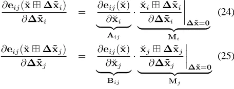
Using the rule for the partial derivatives and exploiting the fact that the Jacobian is evaluated in ∆˜x =0, the non-zero blocks become:

∂eij(˘x⊞∆˜xi)

∂∆˜xi

= ∂eij(˘x) ∂x˘i

| {z } A_ij

· x˘i⊞∆˜xi

∂∆˜xi

_∆˜x

=0 | {z }

M_i

(24)

∂eij(˘x⊞∆˜xj)

∂∆˜x_j =

∂eij(˘x)

∂x˘_j | {z }

B_ij

· x˘j⊞∆˜xj

∂∆˜x_{j ∆˜x}

=0 | {z }

M_j

(25)

Accordingly, one can easily derive from the Jacobian not defined on a manifold of Eq. 17 a Jacobian on a manifold just by multiplying its non-zero blocks with the derivative of the⊞operator computed inx˘i andx˘j.

Fig. 8. A typical robot used in 2D mapping experiments. The platform is a standard ActivMedia Pioneer 2 equipped with a SICK-LMS range finder.

With a straightforward extension of the notation, we can insert Eq. (21) in Eq. (9). This leads to the following linear system:

˜

H ∆˜x∗ = −b˜. (26)

Since the increments∆˜x∗are computed in the local Euclidean surroundings of the initial guessx˘, they need to be re-mapped into the original over-parametrized space by the ⊞operator. Accordingly, the update rule of Eq. (16) becomes

x∗ = ˘x_⊞∆˜x∗. (27)

Thus, formalizing the minimization problem on a manifold consists of first computing a set of increments in a local Euclidean approximation around the initial guess by Eq. (26), and second accumulating the increments in the global non-Euclidean space by Eq. (27). Note that the linear system computed on a manifold representation has the same structure of the linear system computed on an Euclidean space. One can easily derive a manifold version of a graph minimization from a non-manifold version, only by defining an⊞operator and its JacobianMiw.r.t. the corresponding parameter block. Algorithm 2 provides a manifold version of the Gauss-Newton method for SLAM.

The Hessian H˜ of the manifold problem no longer rep-resents the information matrix of the trajectories but of the trajectory increments∆˜x. To obtain the information matrix of the trajectory Algorithm 2 computes H in the original space of the poses x.

V. PRACTICALAPPLICATIONS

In this section we describe some applications of the pro-posed methods. In the first scenario we describe a complete 2D mapping system, and in the second scenario we briefly de-scribe a 3D mapping system and we highlight the advantages of a manifold representation.

A. 2D Laser Based Mapping

Algorithm 2 Manifold version of Algorithm 1. While this al-gorithm has the same computational complexity, it is substan-tially more robust than the non-manifold version, especially in the 3D case.

Require: ˘x = ˘x1:T: initial guess. C = {heij(·),Ωiji}: constraints

Ensure: x∗:new solution,H˘∗ new information matrix // find the maximum likelihood solution

while¬converged do

// Compute the auxiliary JacobiansM1:T over the mani-fold

for allx˘i∈x˘ do

Mi← ˘

x_i⊞∆˜x_i

∂∆˜x_{i ∆˜x}

=0 end for

˜

b←0 H˜ ←0

for allheij,Ωiji ∈ C do

// Compute the Jacobians Aij and Bij of the error function

Aij← ∂

e_ij(x₎

∂x_{i x}

=˘x Bij ←

∂e_ij(x₎

∂x_{j x}

=˘x

// Project the Jacobians through the manifold

˜

Aij←AijMi B˜ij ←BijMj // compute the nonzero Hessian blocks

˜

H[ii]+= ˜ATijΩijA˜ij H˜[ij]+= ˜ATijΩijB˜ij

˜

H[ji] += ˜BTijΩijA˜ij H˜[jj]+= ˜BTijΩijB˜ij // compute the coefficient vector

˜

b[i]+= ˜ATijΩijeij b˜[j]+= ˜BTijΩijeij end for

// keep the first node fixed

H_[11]+= I

// solve the linear system using sparse Cholesky factor-ization

∆˜x←solve( ˜H ∆˜x=−b)˜

// update the parameters for allx˘i∈x˘ do

˘

xi←x˘i⊞∆˜xi end for

end while

x∗←x˘

// the maximum is found, now compute the Hessian in the original space

H∗←0

for allhe_ij,Ω_iji ∈ C do

H_[ii]+= AT

ijΩijAij H[ij] += ATijΩijBij

H[ji] += BTijΩijAij H[jj]+= BTijΩijBij end for

return hx∗,H∗i

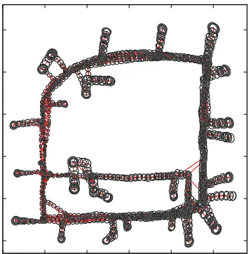
Fig. 9. Intel Research Lab. Left: Unoptimized pose graph overlayed on top of the resulting map. Right: The optimized pose graph and the resulting consistent map.

corresponding to the movements of the platform between consecutive time frames, and 2D laser range data.

The graph is constructed in the following way:

• Whenever the robot moves more than 0.5 meters or

rotates more than 0.5 radians, the algorithm adds a new vertex to the graph and labels it with the current laser observation.

• This laser scan is matched with the previously acquired one to improve the odometry estimate and the corre-sponding edge is added to the graph. We use a variant of the scan-matcher described by Olson [26].

• When the robot reenters a known area after traveling for a long time in a previously unknown region, the algorithm seeks for matches of the current scan with the past measurements (loop closing). If a matching between the current observation and the observation of another node succeeds, the algorithm adds a new edge to the graph. The edge is labeled with the relative transformation that makes the two scans to overlap best. Matching the current measurement with all previous scans would be extremely inefficient and error prone, since it does not consider the known prior about the robot location. Instead, the algorithm selects the candidate nodes in the past as the ones whose3σmarginal covariances contains the current robot pose. These covariances can be obtained as the diagonal blocks of the inverse of a reduced HessianHred.

Hred is obtained from H by removing rows and the

columns of the newly inserted robot pose. Hred is the

information matrix of all the trajectory when assuming fixed the current position.

• The algorithm performs the optimization whenever a loop

closure is detected.

Fig. 10. Pose uncertainty estimate for a real-world data set.

manifolds.

B. 3D Laser Based Mapping

Extending to 3D the SLAM algorithm presented in the previous section is rather straightforward. One has only to replace the 2D scan matching and loop closure detection with their 3D counterparts that operate on 3D point clouds instead than on single laser scans. In our implementation we utilize the popular ICP algorithm [1] and for determining the loop closures we use the algorithm by Steder et al. [29]. Additionally, each node of the graph and each constraint lives inSE(3). Typical outputs of this algorithm are illustrated in Figures 2(a) and (b).

The minimum number of parameters required to represent an element ofSE(3)is 6, a possible choice consists in a 3D translation vector plus the three Euler angles. Utilizing this parametrization leads to Algorithm 1. However, this minimal representation is subject to singularities that can be avoided by utilizing an over-parametrized state space. Alternatively, one can describe the relative perturbations of the optimization problem ∆˜x in a minimal representation while leaving the poses in the original over-parametrized space. This leads to Algorithm 2. In this section we compare these two variants of the optimization algorithm on a pose-graph obtained by a simulated robot. Note that the sparsity pattern of the Hessian is the same in both cases. Furthermore, the time to compute the linear system is negligible compared to the time to solve it. Accordingly, the choice of the parametrization mainly affects the convergence speed, not the time required to perform one iteration. To highlight this effect we show the evolution of the error per iteration during one optimization run by using the two algorithms.

We use a simulated 3D dataset of a robot traveling on the surface of a sphere. The measurements were affected by a significant error, and initializing the system by using the odometry information resulted in the graph illustrated in the left part of Figure 11. Starting from this initial guess we executed the Gauss-Newton Algorithm with and without the manifold linearization, i.e., here by using Euler angles.

Fig. 11. Pose-graph obtained by simulating a robot moving on a sphere. Left: Initial configuration. Right: After optimizing the pose graph the sphere has accurately been recovered by Algorithm 2.

102 103 104 105 106 107 108

0 2 4 6 8 10 12

Iteration

Gauss-Newton (Euler) Gauss-Newton (Manifold)

F

(

x

)

Fig. 12. Evolution of the errorF₍x_{)for Gauss-Newton optimization with} Euler angles and with manifold linearization to the 3D sphere dataset.

Figure 12 shows the evolution of the error during the iterations of the two approaches. First both approaches are able to decrease the error. However, not appropriately considering the singularities leads to a divergence of Algorithm 1 while Algorithm 2 converges to the right solution.

VI. CONCLUSIONS

In this paper we presented a tutorial on graph-based SLAM. Our aim was to provide the reader with sufficient details and insights to allow for an easy implementation of the proposed methods. The algorithms presented in this paper can be used as a building blocks of more sophisticated methods, however optimized implementations of these algorithms can deal with surprisingly large problems.

REFERENCES

[1] Paul J. Besl and Neil D. McKay. A method for registration of 3-d shapes. IEEE Transactions on Pattern Analysis and Machine Intelligence, 14(2):239–256, 1992.

[2] M. Bosse, P. M. Newman, J. J. Leonard, and S. Teller. An ATLAS framework for scalable mapping. In Proc. of the IEEE Int. Conf. on

Robotics & Automation (ICRA), pages 1899–1906, 2003.

[3] J.A. Castellanos, J.M.M. Montiel, J. Neira, and J.D. Tard´os. The SPmap: A probabilistic framework for simultaneous localization and map build-ing. IEEE Transactions on Robotics and Automation, 15(5):948–953, 1999.

[4] T. A. Davis. Direct Methods for Sparse Linear Systems. SIAM, Philadelphia, 2006. Part of the SIAM Book Series on the Fundamentals of Algorithms.

[5] F. Dellaert and M. Kaess. Square root SAM: Simultaneous location and mapping via square root information smoothing. Int. Journal of Robotics

Research, 2006.

[6] C. Estrada, J. Neira, and J.D. Tard´os. Hierachical SLAM: Real-time accurate mapping of large environments. IEEE Transactions on

[7] R. Eustice, H. Singh, and J.J. Leonard. Exactly sparse delayed-state filters. In Proc. of the IEEE Int. Conf. on Robotics & Automation (ICRA), pages 2428–2435, Barcelona, Spain, 2005.

[8] U. Frese, P. Larsson, and T. Duckett. A multilevel relaxation algorithm for simultaneous localisation and mapping. IEEE Transactions on Robotics, 21(2):1–12, 2005.

[9] G. Grisetti, C. Stachniss, and W. Burgard. Improved techniques for grid mapping with rao-blackwellized particle filters. IEEE Transactions on

Robotics, 23(1):34–46, 2007.

[10] G. Grisetti, C. Stachniss, and W. Burgard. Non-linear constraint network optimization for efficient map learning. IEEE Transactions on Intelligent

Transportation Systems, 2009.

[11] J.-S. Gutmann and K. Konolige. Incremental mapping of large cyclic environments. In Proc. of the IEEE Int. Symposium on Computational

Intelligence in Robotics and Automation (CIRA), 1999.

[12] D. H¨ahnel, W. Burgard, D. Fox, and S. Thrun. An efficient FastSLAM algorithm for generating maps of large-scale cyclic environments from raw laser range measurements. In Proc. of the IEEE/RSJ Int. Conf. on

Intelligent Robots and Systems (IROS), pages 206–211, Las Vegas, NV,

USA, 2003.

[13] D. H¨ahnel, W. Burgard, B. Wegbreit, and S. Thrun. Towards lazy data association in slam. In Proc. of the Int. Symposium of Robotics Research

(ISRR), pages 421–431, Siena, Italy, 2003.

[14] C. Hertzberg. A framework for sparse, non-linear least squares problems on manifolds. Master’s thesis, Univ. Bremen, 2008.

[15] A. Howard, M.J. Matari´c, and G. Sukhatme. Relaxation on a mesh: a formalism for generalized localization. In Proc. of the IEEE/RSJ

Int. Conf. on Intelligent Robots and Systems (IROS), 2001.

[16] M. Kaess, A. Ranganathan, and F. Dellaert. iSAM: Fast incremental smoothing and mapping with efficient data association. In Proc. of the

IEEE Int. Conf. on Robotics & Automation (ICRA), Rome, Italy, 2007.

[17] K. Konolige. A gradient method for realtime robot control. In Proc. of

the IEEE/RSJ Int. Conf. on Intelligent Robots and Systems (IROS), 2000.

[18] K. Konolige, J. Bowman, J. D. Chen, P. Mihelich, M. Calonder, V. Lepetit, and P. Fua. View-based maps. International Journal of

Robotics Research (IJRR), 29(10), 2010.

[19] K. Konolige, G. Grisetti, R. K¨ummerle, W. Burgard, B. Limketkai, and R. Vincent. Sparse pose adjustment for 2d mapping. In Proc. of the

IEEE/RSJ Int. Conf. on Intelligent Robots and Systems (IROS), 2010.

[20] J.M. Lee. Introduction to Smooth Manifolds, volume 218 of Graduate

Texts in Mathematics. Springer Verlag, 2003.

[21] F. Lu and E. Milios. Globally consistent range scan alignment for environment mapping. Autonomous Robots, 4:333–349, 1997. [22] M. Montemerlo, S. Thrun, D. Koller, and B. Wegbreit. FastSLAM: A

factored solution to simultaneous localization and mapping. In Proc. of

the National Conference on Artificial Intelligence (AAAI), pages 593–

598, Edmonton, Canada, 2002.

[23] J. Neira and J.D. Tard´os. Data association in stochastic mapping using the joint compatibility test. IEEE Transactions on Robotics and

Automation, 17(6):890–897, 2001.

[24] A. N¨uchter, K. Lingemann, J. Hertzberg, and H. Surmann. 6D SLAM with approximate data association. In Proc. of the Int. Conference on

Advanced Robotics (ICAR), pages 242–249, 2005.

[25] E. Olson. Robust and Efficient Robotic Mapping. PhD thesis, MIT, Cambridge, MA, USA, June 2008.

[26] E. Olson. Real-time correlative scan matching. In Proc. of the IEEE

Int. Conf. on Robotics & Automation (ICRA), 2009.

[27] E. Olson, J. Leonard, and S. Teller. Fast iterative optimization of pose graphs with poor initial estimates. In Proc. of the IEEE Int. Conf. on

Robotics & Automation (ICRA), pages 2262–2269, 2006.

[28] R. Smith, M. Self, and P. Cheeseman. Estimating uncertain spatial realtionships in robotics. In I. Cox and G. Wilfong, editors, Autonomous

Robot Vehicles, pages 167–193. Springer Verlag, 1990.

[29] B. Steder, G. Grisetti, and W. Burgard. Robust place recognition for 3D range data based on point features. In Proc. of the IEEE Int. Conf. on

Robotics & Automation (ICRA), 2010.

[30] C.J. Taylor and D.J. Kriegman. Minimization on the Lie group SO(3) and related manifolds. Technical Report 9405, Yale University, 1994. [31] S. Thrun, Y. Liu, D. Koller, A.Y. Ng, Z. Ghahramani, and H.

Durrant-Whyte. Simultaneous localization and mapping with sparse extended information filters. Int. Journal of Robotics Research, 23(7/8):693–716, 2004.

[32] S. Thrun and M. Montemerlo. The graph SLAM algorithm with applications to large-scale mapping of urban structures. Int. Journal

of Robotics Research, 25(5-6):403, 2006.

[33] R. Triebel, P. Pfaff, and W. Burgard. Multi-level surface maps for outdoor terrain mapping and loop closing. In Proc. of the IEEE/RSJ

Int. Conf. on Intelligent Robots and Systems (IROS), 2006.

APPENDIX

In the following we will provide the definitions and the derivations for the Jacobians to implement the suggested algorithm. Due to space limitations we do not expand the Jacobians in the 3D case. However, these Jacobians can either be computed numerically or by using a computer algebra system.

Error Functions and Jacobians for the 2D case

The basic entities in the 2D case are defined as

x⊤_i = (t⊤_i , θi) (28)

z⊤_ij = (t⊤ij, θij) (29)

where ti andtij are 2D vectors and θi and θij are rotation angles which are normalized to[−π, π). The error function is

eij(x) =

R⊤_ij(R⊤

i (tj−ti)−tij)

θj−θi−θij

, (30)

where Ri and Rij are the 2×2 rotation matrices of θi and

θij with the following structure

Ri =

cos(θi) −sin(θi)

sin(θi) cos(θi)

. (31)

The Jacobians of the error function are

Aij=

∂eij(x)

∂x_i =

−R⊤_ijR⊤_i R⊤_ij∂R⊤i

∂θi (tj−ti)

0⊤ −1

!

(32)

Bij=

∂eij(x)

∂xj

=

R⊤_ijR⊤_i 0

0⊤ 1

. (33)

The ⊞operator is defined as

x⊞∆˜x=x+∆˜x (34)

The angles are normalized to [−π, π) after applying the increments. The Jacobians of the manifold in the 2D case evaluate to the identity matrix:

Mi=

x_i⊞∆˜x_i ∂∆˜xi

_∆˜x

=0

=I3 (35)

Mj=

xj⊞∆˜xj

∂∆˜xj

_∆˜x

=0

=I3 (36)

.

Error Functions for the 3D case

The basic entities in the 3D case are defined as

x⊤_i = (t⊤_i ,q⊤_i ) (37)

z⊤_ij = (t⊤_ij,q⊤_ij), (38)

where q denotes the unit quaternionq⊤ = (qx, qy, qz, qw)⊤, i.e., kqk= 1. The error function is

eij(x) = z−ij1⊕(x

−1

i ⊕xj)

where ⊕is the motion composition operator

x_i⊕x_j =

qi(tj)

qi·qj

(40)

and the operator(·)[1:6]selects the first 6 elements of its vector argument.

The Jacobians of the error function are:

A_ij= ∂eij(x) ∂xi

(41)

Bij=

∂eij(x)

∂xj

. (42)

The ⊞ operator maps ∆˜x⊤_i = (∆˜t⊤_i ,∆˜q⊤_i ) to the original space

xi⊞∆˜xi = xi⊕





∆˜ti

∆˜q_i p

1− k∆˜q_ik2 

, (43)

where ∆˜ti denotes the translation and ∆˜q⊤ =

(∆qx,∆qy,∆qz)⊤ is the vector part of the unit quaternion representing the 3D rotation and thus k∆˜q_ik ≤ 1. The Jacobians of the manifold in the 3D case are given by

Mi=

xi⊞∆˜xi

∂∆˜x_{i ∆˜x}

=0

(44)

Mj=

xj⊞∆˜xj

∂∆˜x_{j ∆˜x}

=0