2003_NZsunsets_AO.pdf

Novaya Zemlya effect and sunsets

Siebren Y. van der Werf, Gu¨nther P. Ko¨nnen, and Waldemar H. Lehn

Systematics of the Novaya Zemlya共NZ兲effect are discussed in the context of sunsets. We distinguish full mirages, exhibiting oscillatory light paths and their onsets, the subcritical mirages. Ray-tracing examples and sequences of solar images are shown. We discuss two historical observations by Fridtjof Nansen and by Vivian Fuchs, and we report a recent South Pole observation of the NZ effect for the Moon. © 2003 Optical Society of America

OCIS code: 010.4030.

1. Introduction

The image of the low Sun that we see depends criti-cally on the temperature profile in the lowest few hundred meters above ground or sea level. For a standard temperature profile, with a constant tem-perature gradient, the Sun just flattens but is not otherwise distorted.

When there is in addition a warm surface layer over the ground or the water, an observer above this layer may see an inferior mirage, the desert mirage: A second image of the Sun appears below the first and looks like its reflection. As the Sun sinks lower, the two images merge together to form the familiar omega shape, and finally the Sun’s last light disap-pears in a green flash.

Cold surface layers can produce various forms of distortion. The most dramatic example is the No-vaya Zemlya共NZ兲effect, an arctic mirage over huge distances, caused by a strong temperature inversion. Here the image of the Sun may be rectangular and can be split into several horizontal pieces.

To understand these effects and to reproduce them by calculation, one has to know how the refraction varies with the apparent altitude. Given a model of the atmosphere that allows the refractive index to be

found for all heights, the refraction can be established by means of tracing the light’s path backwards from the eye of the observer to the object from which it was emitted. In this paper we present such models and the ray-tracing calculations that go with them.

The emphasis of the present analysis will be on the NZ mirage. To show how the NZ mirage fits in the family of sunsets, we shall also discuss the standard atmosphere and the desert mirage.

Ray-tracing calculations are based on the curva-ture of the light’s path, defined as the inverse of its radius of curvature: c ⬅ 1兾r. However, for the sake of discussion we find it convenient to express the curvature in a local Cartesian frame and measure height from the Earth’s surface upwards and the hor-izontal coordinate as distance along it. We show in Section 2 that for near-horizontal rays this terrestrial ray curvature is justcT⫽1兾r⫹1兾RE, whereREis the Earth’s radius.

For a normal atmosphere, the temperature gradi-ent is approximately ⫺0.006 °C兾m, and the light’s radius of curvature is⬃6 times larger than that of the Earth. Upon backward tracing, a ray that is hori-zontal at the observer’s position is bent downwards, but the Earth’s surface curves away faster, and the ray escapes. To the observer,cTis then positive, and he would say that the ray is bent away from the Earth.

When, however, there exists a strong temperature inversion, where in some height interval the vertical temperature gradient exceeds the value of 0.11 °C兾m, cT becomes negative in that interval, and near-horizontal light rays in this region are bent back towards the Earth. This may give rise to oscillatory light paths, which is the characteristic of the NZ mi-rage. In the following we shall use the phrases NZ mirage and NZ effect indiscriminately.

We discuss the NZ mirage for the situation of an S. Y. van der Werf_共[email protected]_兲is with the Kernfysisch

Ver-sneller Instituut, University of Groningen, Zernikelaan 25, 9747AA Groningen, The Netherlands. G. P. Ko¨nnen_共konnen@ knmi.nl_兲is with the Royal Netherlands Meteorological Institute, P.O. Box 201, 3730AE de Bilt, The Netherlands. W. H. Lehn

共[email protected]_兲is with the Department of Electrical and Computer Engineering, University of Manitoba, Winnipeg R3T 5V6, Canada.

Received 29 November 2001; revised manuscript received 20 March 2002.

observer below and above the inversion and distin-guish these two situations as the superior and the inferior NZ mirages, respectively. In addition, we study the onsets to these effects, which we denote as subcritical NZ effects, and finally we investigate their color dispersion. The subcritical inferior mirage has been named the “mock mirage” by Younget al.1

Most of the classical observations 共Barents,2,3

Nansen,4_Shackleton5兲_{were doubtlessly made for an}

overhead inversion and should be classified as supe-rior mirages. In this paper we give a short discus-sion of the observations of Nansen and of the less-known observation of Sir Vivian Fuchs,6_{made on 14}

August 1957 at Shackleton Base. The latter case may well have been an example of an inferior NZ mirage. An extensive analysis of Barents’ observa-tion, made on Novaya Zemlya in 1597, is presented in a separate paper in this issue.7

This paper is organized as follows: Section 2 deals with ray tracing and the description and parametri-zation of the atmosphere. In Section 3 we make a rough classification of the different types of sunset and indicate how the NZ effect fits into this family. Section 4 gives a more detailed analysis of both the superior and the inferior NZ mirages. The observa-tions of Nansen and Fuchs are discussed in Section 5. In Section 6 we present the first recording of the NZ effect for the Moon, an observation made at U.S. Amundsen–Scott South Pole Station on 7– 8 May 1998. Section 7 contains a summary. In order not to interrupt the reading, the derivation of some equa-tions that are less commonly known or used are de-ferred to Appendix A.

2. Model of the Atmosphere and Ray Tracing

The techniques used in this paper are the same as used by Van der Werf.8 _{Here we generalize these}

procedures so that they will be applicable to non-standard atmospheres that also have horizontal tem-perature and pressure gradients. Below we sketch these generalizations. Derivations are given in Ap-pendix A.

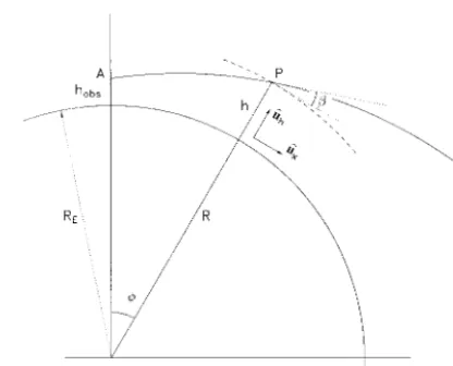
The backward ray-tracing procedure is illustrated in Fig. 1. It requires that one should be able to evaluate the curvature at any arbitrary point P of the ray. The curvature of a light ray in the atmosphere is proportional to the logarithmic gradient of the re-fractive index, n. When this depends not only on height,h, but also onx, the distance along the Earth’s surface, one has at P with polar coordinates 共R, ␾兲 共see Appendix A兲,

1 r⫽

1

n共h,x兲

冋

⳵n共h, x兲

⳵h ⫺sin共␤兲

⳵n共h,x兲 ⳵x

册

(1)

whereris the light ray’s radius and␤ ⫽arctan共dh兾 dx兲is the tilt of the ray relative to the local horizontal. The curve is concave relative to the Earth’s center whenr⬍0, convex whenr⬎ 0.

In a local Cartesian coordinate frame, wherehand

xare distances above and along the Earth’s surface, the light ray’s curvature is given by

cT共h, ␤兲⬅

d2_h兾dx2

关1⫹共dh兾dx兲2_兴3兾2

⫽1

r⫹ 1

Rcos共␤兲关1⫹sin

2共␤兲兴, (2)

where R ⫽ RE ⫹ h. In the following we shall call this the terrestrial ray-curvature. For near-horizontal rays, close to the Earth’s surface the rays obey to a good approximation the relation

d2_h

dx2⬇

1 r⫹

1 RE

⫽cT共h,␤⫽0兲. (3)

In this study we shall be concerned with rays that are always very nearly horizontal, and in the follow-ing we shall often abbreviate the terrestrial ray-curvature’s notation to justc_T, understanding that it still depends on height.

Exact ray-tracing calculations are most easily per-formed in polar coordinates共R,␾兲around the Earth’s center. Any curve obeys8

dR

d␾⫽Rtan共␤兲, (4)

d␤ d␾⫽1⫹

1 r

R

cos共␤兲. (5)

As above,␤is the tilt angle of the ray relative to the local horizontal, or, stated differently, it is the com-plement of the angle between the position vector and the curve at the point共R,␾兲.

Equations共4兲and共5兲form a system of two coupled first-order differential equations forR and␤with␾ as independent variable. They are amenable in this Fig. 1. Illustration of the ray-tracing procedure. The observer is in A at heighthobsabove sea level. The ray enters from the right

and passes through point P, with polar coordinates_共R,_␾兲at height

habove sea level, where its angle with the local horizontal is_␤. At P a local frame of reference is defined with unit vectorsuˆx共

form to numerical integration, e.g., by the fourth-order Runge–Kutta method, under the condition that in every point the radius of curvature,r⫽r共R,␤,␾兲, can be evaluated.

This scheme is more general and flexible than the conventional method of Auer and Standish9 _and

needs no additional provisions to handle negative ap-parent altitudes and oscillatory ray trajectories. Moreover, it may be used without modifications when the atmosphere exhibits horizontal temperature and pressure gradients, such as we shall need in this paper.

The index of refraction,n, follows from共see Appen-dix A兲

n共h,x兲⫽1⫹A共␭兲P共0,x兲 T共h,x兲

⫻exp

冋

兰

0

h_g共_h⬘兲

g共0兲 dh⬘

T共h⬘, x兲

册

Here,T共h,x兲is the temperature profile;P共0,x兲, the atmospheric pressure at sea level; andg共h兲, the grav-itational acceleration at height h. A共␭兲 depends slightly on wavelength. Using the wavelength de-pendence of dry air as given in the Handbook of

Chemistry and Physics,10_{one finds the following}

val-ues for green, yellow, and red light: A共520 nm兲 ⫽ 7.8998 10⫺5K兾hPa共green兲,A共580 nm兲 ⫽7.8686 10⫺5 K兾hPa共yellow兲, andA共650 nm兲 ⫽7.8434 10⫺5_K兾hPa

共red兲. Further,B⫽ 3.4177 10⫺2°C兾m.

To findn共h,x兲, it is necessary to have a functional description of T共h, x兲 that will be suitable for ray tracing and flexible enough to describe the character-istics of the atmospheres that cause the NZ effect and the desert mirage. We use a temperature profile that is based on the U.S. standard atmosphere of 1976 共US1976兲. To allow for a free choice of the temperature at sea level,T0, the height of the

tropo-sphere,H_T, is made variable. Also, the atmospheric pressure at sea level, P0, is made adjustable. The

thus modified US1976 atmosphere has been denoted as MUSA76.8 _{We may append to this MUSA76}

at-mosphere a warm or cold layer, for which we use an analytical form, borrowed from the theory of the elec-tron gas, where it is known as the Fermi distribution. The same function is used in nuclear physics, where it is encountered as the Woods–Saxon potential:

T共h, x兲⫽TMUSA76共h兲⫺⌬T共x兲

⫹ ⌬T共x兲

1⫹exp兵⫺关h⫺hciso共x兲兴兾a共x兲其

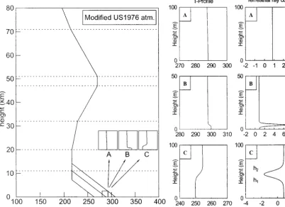
. (7) Fig. 2. Left, the modified US1976 atmosphere, shifted in the troposphere to match the sea-level temperature. At low heights an additional temperature profile may be added, indicated by the insets and shown enlarged in the middle diagrams: A, standard atmosphere, sea-level temperatureT0⫽288.15 K共15 °C兲. B, a warm layer as could produce a desert mirage for an observer above it.

T0⫽300.15 K共27 °C兲,hciso⫽4 m,a⫽0.5 m, and⌬T⫽ ⫺2 °C. C, a cold layer as could produce the NZ effect. T0⫽250.15 K共⫺23 °C兲,

hciso⫽45 m,a⫽4 m, and⌬T⫽ 5 °C. The diagrams on the right show the corresponding terrestrial ray-curvatures in the lower

Here, h_ciso共x兲 is the height of the isotherm about which the added temperature profile is centered. ⌬T共x兲is the temperature jump across the inversion, and the diffuseness parameter a共x兲 determines the width of the jump.

Figure 2 shows the MUSA76 atmosphere. The in-sets, shown enlarged in the second column, indicate the cases of A, no addition; B, an additional warm layer; and C, an additional cold layer. The corre-sponding terrestrial ray-curvatures are shown in the third column.

3. Rough Classification of Sunsets

The image of the Sun can be found when for each true 共geometric兲altitude,␾共⬁兲, the apparent altitude,␤, is known. The functional relationship between them can be named the transformation curve.

A rough classification of sunsets is made in this section, taking as examples the three temperature profiles shown in Fig. 2. For each of them we give an example of ray tracing, the transformation curve, and a sequence of images for the setting Sun. All ray tracings are done up to a height of 85 km.

If there were no atmosphere at all, the path of a light ray would be straight and a light-emitting body would be in the direction in which it is seen. The transformation curve would be simply given by␤ ⫽ ␾共⬁兲. The image of the Sun would be perfectly round, progressively chopped off from below by the horizon as it sinks.

A. Standard US1976 Atmosphere

Ray tracing for the standard US1976 atmosphere is shown in Fig. 3. The observer’s height is 15 m.

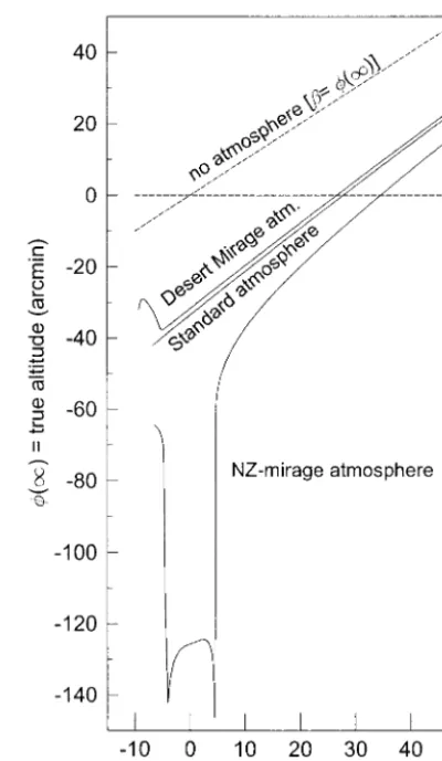
Light paths for different apparent altitudes are shown in the first 100 m. The pattern is quite regular: Rays do not cross, and the higher the apparent altitude, the higher also the true altitude. The transformation curve for the standard atmo-sphere is shown in Fig. 4, along with those for the desert mirage and the NZ effect, discussed in the following subsections. It is depressed relative to the hypothetical case of no atmosphere. The difference between them is the atmospherical refraction, and this increases with decreasing apparent altitude. The latter may become negative because the observer is at a certain height above sea level. The lowest apparent altitude,␤_min, is the one for which the ray just grazes sea level at its lowest height. This de-fines the apparent horizon, and ⫺␤_min is called the horizon dip.

The sequence of the Sun’s images on top of Fig. 3 shows a flattening that gives a nearly perfect ellipti-cal shape. The ratio of the vertical and the horizon-tal axes equals d␤兾d␾共⬁兲, which is the Jacobian of the transformation from the true to the apparent alti-tude. This may in turn be related to the refraction, Fig. 3. Light paths for the standard atmosphere_共inset A of Fig. 2_兲

traced backwards from an observer’s height at 15 m, up to an apparent altitude of 50_⬘. The corresponding images of the Sun are shown along the top, for equidistant steps in altitude. The scale of the horizontal distance along the Earth_共xaxis_兲has been compressed by a factor 500 relative to theyaxis.

which is defined by ␰ ⬅ ␤ ⫺ ␾共⬁兲. It is then conve-nient to introduce the flattening as

flattening⬅hor.axis⫺vert.axis

hor.axis ⫽

d关␾共⬁兲⫺␤兴 d␾共⬁兲

⫽⫺ d␰

d␾共⬁兲. (8)

Since the refraction increases faster than linear with decreasing true altitude, the flattening increases as the Sun sinks. Its approximate value at apparent altitude ␤ ⫽0 can easily be calculated analytically 共see Appendix A兲and gives, expressed in terms of the terrestrial ray-curvature,

flattening共␤⫽0兲⬇1⫺REcT共␤⫽0兲

⫽A共␭兲P0RE

T02

冋冉

dT

dh

冊

册

constant from sea level up to the height of the ob-server, under the condition that 0ⱕREcT共␤ ⫽0兲ⱕ 1. Inserting the parameters for the US1976 stan-dard atmosphere, except the temperature gradient, gives

flattening共␤⫽0兲⬇0.21

冋

冉

dh

冊

册

the flattening has a value of 0.17.

B. Desert Mirage

We now consider a warm layer causing a desert mi-rage. The observer will again be at a height of 15 m above sea level. The parameters are as in Fig. 2, case B: The warm layer has a temperature jump ⌬T ⫽ ⫺2 °C. The diffuseness is a ⫽ 0.5 m, and hence more than 90% of this jump is confined in an interval⌬h⬇6a⫽3 m around the central isotherm at h_ciso ⫽ 4 m关see Eq. 共7兲兴. In the vicinity of this central isotherm the共negative兲temperature gradient is so strong that the ratioP兾T, and hence the density, increases with height: One has a density inversion. The condition for this to occur is

dT

dhⱕ⫺B⫽⫺3.4 10

⫺2

°C兾m. (11)

The curvature, 1兾r, then becomes positive, and for the terrestrial ray-curvature, one hascT⬎1兾RE, as is shown in Fig. 2, case B.

Rays drawn from the observer’s eye at positive ap-parent altitude travel through an altogether normal atmosphere. But rays seen at negative apparent al-titude that come near the density inversion receive an upward sweep in this region, resulting in a smaller refraction. The effect is clear from Fig. 5, which shows that it is possible for rays at negative

apparent altitude to cross other rays at less negative apparent altitude.

The effect of adding a warm surface layer to the 共standard兲atmosphere on the transformation curve is shown in Fig. 4. The refraction does not increase all the way with decreasing apparent altitude, but suddenly bends upwards again. In this region one has d␾共⬁兲兾d␤ ⬍ 0, meaning that the image is mir-rored.

The lowest point of the transformation curve marks the vanishing line where the upright image and the mirrored image merge and finally disap-pear in a point as the Sun sets. This is illustrated by the sequence of images in Fig. 5. The color dispersion is such that the transformation curve for green light lies lower than that for red light. This color dispersion is largest on the vanishing line, and a pronounced green flash may be seen when the air is clean enough.

C. Novaya Zemlya Effect

Next we consider the cold layer as shown in Fig. 2, case C. The observer is again at 15 m above sea level. Overhead for him is a temperature inversion that is centered aroundhciso ⫽ 45 m. The

temper-ature jump is⌬T⫽5 °C, and the diffuseness param-eter isa⫽4 m. Thus, whereas for the desert mirage the observer is above the region of the largest tem-perature gradient, he now is below it.

From Fig. 2, case C, one notes that the terrestrial ray-curvature, cT, is negative on a height interval aroundhciso. For this to occur, the condition is

dT dh⬎

T共h兲2 A共␭兲P共h兲RE

which implies a temperature gradient that is typi-cally larger that 0.11 °C兾m.

Denote ash₁the lowest level in Fig. 2, case C, for which we have cT ⫽ 0, so that at h ⫽ h1: 1兾r ⫽

⫺1兾R_E. Then, by relation共3兲, and expandingc_T共h兲 aroundh1up to first order, we have

d2_共h⫺h 1兲

dx2 ⫽

冉

dcT dh

冊

1

共h⫺h1兲. (13)

Ath⫽h₁,共dc_T兾dh兲is negative so that relation共12兲 allows for harmonic oscillations around the heighth1.

This solution provides the schematic explanation of the NZ effect.

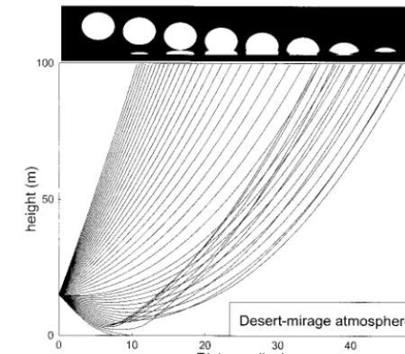
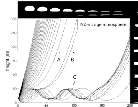
Figure 6 illustrates the ray-tracing results. Rays of sufficiently high apparent altitude, indicated by A, break through the inversion layer, and the higher␤, the less the effect of the inversion. Also rays that, upon backward tracing, start out from the observer on a sufficiently negative altitude will on their up-ward course pass through the inversion with little disturbance共rays indicated by B兲. In between there is an interval of␤values, symmetric around the true horizon, where the rays enter the inversion zone at small enough angles to be trapped 共rays C兲. They then follow oscillatory paths until the inversion weakens sufficiently that it can no longer sustain the oscillations. The methods for achieving this weak-ening of the inversion in the context of the ray-tracing formalism are discussed in Section 4.

In the interval of␤values, for which the NZ effect occurs, the refraction increases dramatically, and the corresponding true altitudes, ␾共⬁兲, are much de-pressed. The transformation curve of the present example is included in Fig. 4.

The images of the sunsets are shown also in Fig. 6. Along the top of the figure one first sees the images of the Sun at positive apparent altitudes 共rays A兲. When ␤ decreases, the part where the rays become oscillatory共rays C兲is missing, and the image strongly flattens at the bottom. Next, when the Sun is low enough to match the rays of strongly negative␤ val-ues共rays B兲, the corresponding共mirrored兲image ap-pears. In between is the gap from which the rays C are missing, which is sometimes called Wegener’s blind band.

But when the Sun has sunk far enough, the situ-ation reverses: The rays from categories A and B are now missing, but those from C, which correspond to a much lower true altitude, ␾共⬁兲, will contribute when the Sun matches these altitudes. This is the depressed part of the transformation curve. The im-ages are highly distorted and pass through a rectan-gular phase and phases where the image is split into several disjunct components. These are shown in Fig. 6 on the right-hand side.

4. Systematics of the Novaya Zemlya Effect

In this section we investigate the NZ effect in more detail. In particular, we study the role of the height of the observer and the strength of the inversion, as embodied in the temperature jump. Also, we study

its color dispersion. To do so, we adopt a tempera-ture inversion appended, as before, from the MUSA76 atmosphere. Its central isotherm will be at a heighth_ciso⫽40 m, with a diffuseness parameter of a⫽ 3 m. The sea-level temperature is taken as T₀⫽260 K in all cases. We shall place the observer below the inversion, ath⫽15 m and above it, ath⫽ 45 m and distinguish these cases as superior and inferior mirages, respectively. When the tempera-ture jump is strong enough to force at least part of the rays into oscillatory paths, we shall speak offull mi-rages. If the temperature jump is 共just兲not strong enough to achieve this, we will denote them as sub-critical mirages.

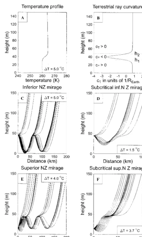
In its top panels Fig. 7 shows the temperature profile and the terrestrial curvature for such an in-version for a temperature jump of⌬T ⫽ 5 °C. The other panels show the tracing examples for the sub-critical and full mirages, both inferior and superior.

As mentioned above, it is necessary for a full mi-rage to let the inversion weaken away from the ob-server such that the backwards traced rays are allowed to escape upwards through the inversion. There are two obvious ways to achieve this: 共1兲by making⌬Tdependent on distance and making it de-crease in a convenient way and 共2兲 by making the diffuseness parameter, a, depend on distance and letting it increase with distance, decreasing in this way the temperature gradient across the inversion. Mathematically, the two methods are rather similar, and we have chosen the second method. For the Fig. 6. Light paths for the NZ mirage atmosphere共inset C of Fig. 2兲, observer’s height at 15 m, and corresponding images of the Sun. The strong temperature inversion is here above the observer共 su-perior mirage兲. For apparent altitudes,␤, larger than a given value, the backwards traced rays共indicated by A兲break through the inversion. Also, rays of sufficient negative␤, which共just兲miss the ground, break through the inversion on their upward course

共indicated by B兲. In a limited range of apparent altitudes, around

dependence of the diffuseness on distance we adopt the following form:

a共x兲⫽a共0兲, xⱕx0, (14)

a共x兲⫽a共0兲关1⫹␣共x⫺x0兲2兴, x⬎x0, (15)

wherex0and␣are parameters that may be adjusted

for each case separately. In all the calculations, shown in this section,x0has been set at 50 km. For

all subcritical mirages the rays escape already before 50 km, and the value of the parameter␣is irrelevant in these cases. However, since␣determines how fast the inversion weakens with distance beyondx0, the ray

tracing for the full mirages depends sensitively on its value. The calculations of the full inferior mirage 共⌬T⫽5.0 °C兲and the full superior mirage共for⌬T⫽ 4.0 °C兲have been made with a value␣ ⫽0.0001. For

the case of the superior mirage with the much stronger inversion共⌬T⫽7.0 °C兲,␣ ⫽0.0004 was used.

For an inferior mirage to show oscillatory paths the observer must be within the region where the terres-trial ray-curvature is negative. With reference to Fig. 7B, he must be abovehcisoto classify the mirage

as inferior, but belowh₂, wherec_T⫽0. If he is above h2, a ray traced backwards starting out at a negative

apparent altitude will on its following upward course reach the observer’s height again but this time with the opposite apparent altitude and thus escape. If he is, however, belowh2, rays within some range of␤

values will have oscillatory paths. This range in-creases as the observer lowers his position.

Also for a superior mirage the height of the ob-server affects the image. When he has a low posi-tion, the ground or sea level limits the range of ␤ values that can be ducted by the inversion to the negative side. But by the same mechanism, also rays at positive apparent altitude are chopped off when, after one oscillation, they return at the observ-er’s height, this time on a downward course. Hence the range of ␤ values that contribute to the image increases with height above the ground.

The transformation curves are shown in Fig. 8 for red 共650 nm兲, yellow 共580 nm兲, and green 共520 nm兲 light. One notes the similarity between the inferior and the superior mirages: For a small temperature jump, such that the mirages are subcritical共Figs. 7D and 7F兲, rays that are horizontal in the region where the temperature gradient is largest tend to stick to this region. In their transformation curves this effect shows up as a narrow depression, deepening and broadening as⌬Tis made to increase. The transfor-mation curves for the subcritical NZ mirages, both superior and inferior, show some similarity to that of the desert mirage共see Fig. 4兲. Also here, the region of positive apparent altitude, to the right of the depres-sion, gives an upright image. Directly to the left of the dip, the transformation curves slope down and pro-duce an inverted image. In the dip itself the color dispersion is large, especially for the subcritical supe-rior mirage. Both the inferior and the superior mi-rages, when just subcritical, can produce a pronounced green flash. Typical sunset sequences are shown in Fig. 9.

The subcritical superior and the subcritical inferior NZ mirages also share with the desert mirage the feature that the transformation curves may exhibit a maximum at negative apparent angles. For this to occur the observer should be at a high enough posi-tion, else this maximum will be chopped off by the horizon. When the sinking Sun just touches this maximum, it will show the red light first, and the satellite image appears as a red flash.

When⌬Tbecomes large enough to force some of the rays into oscillatory paths, the dips in the transfor-mation curves are drastically depressed and widened. The regular sunset now has a blind band, as the top row of images in Fig. 6 shows. When the Sun sinks further, it will reappear when its true alti-tude matches the depressed central part of the Fig. 7. A, Temperature profile of an inversion,⌬T⫽5.0 °C,

cen-tered aroundhciso⫽40 m with a width parametera⫽3 m. B,

Terrestrial ray-curvature, showing the heightsh1andh2, between

which cT is negative. For an observer at h ⫽ 45 m: C, full

inferior NZ mirage,⌬T⫽5.0 °C. D, Subcritical inferior NZ mi-rage,⌬T⫽1.5 °C. For an observer ath⫽15 m: E, full superior NZ mirage,⌬T⫽4.0 °C. F, Subcritical superior NZ mirage,⌬T⫽

transformation curve, and this time it is seen inside what earlier was the blind band. Also for these full mirages sunset sequences are shown in Fig. 9.

5. The Observations of Nansen and Fuchs

On 16 February 1894 Fridtjof Nansen saw the NZ effect, at 80° 01⬘ N and approximately 135° E. A drawing, made by him, is shown in Fig. 10. Nansen described it as follows:

At first the image was a flattened glowing stripe of fire at the horizon. Then two stripes grew out of it, one above the other with a dark space in be-tween. After climbing up the main mast I saw four or even five of such horizontal lines, all equally long such as one would imagine a dull-toned red and square sun, with dark horizontal stripes. 共Ref. 4兲

The true altitude of the Sun at local noon was ⫺2° 22⬘. Nansen’s description comes close to the images of the superior NZ effect, analyzed before for ⌬T ⫽ 7 °C, of which the images are shown in Fig. 9, column 3. The fact that the image grew in width when he climbed up the mast shows that its width was limited by the height of the observer above the ground and, as explained in Section 4, indicates that it must have been a superior mirage.

On 14 August 1957 the NZ effect was observed from Shackleton Base, 77° 57⬘S, 37° 17⬘W. At local noon the Sun’s true altitude was ⫺2° 17⬘. Fuchs6

described the event as follows:

Then a fraction of the sun’s disc appeared again, flickered and disappeared. For some time it came and went, the greatest elevation revealing about one tenth of its orb. Sometimes as it reappeared a red flash seemed to shoot out and pulsate along the horizon. 共Ref. 6兲

Here we possibly have an example of an inferior NZ mirage, at the edge between subcritical and oscillatory. This would explain the small height of the image. See for comparison the images of Fig. 9, fourth column. Further, the observer’s position was rather high: 60 m above sea level. And finally, the red flash, “pulsat-ing along the horizon,” indicates that the light rays within a small apparent altitude range did skim the ice at the lowest point of their path when going from a subcritical into a full mirage. See also the ray tracing for our analysis of an inferior NZ mirage in Fig. 7C. If the inversion had been overhead, then, for a just crit-ical inversion, the rays would never have come much lower than the height of the observer himself, and could not have been reflected off the ice.

6. Observation of the Novaya Zemlaya Effect for the Moon

through a distorted phase and transformed into its normal appearance at approximately 07:30 UT on 8 May, when its true altitude was 1° 03⬘.5.

Warmer air was coming in, and the ground tem-peratures on 8 May were ⫺68 °C 共0 UT兲, ⫺66 °C 共6 UT兲,⫺60 °C共12 UT兲at a pressure of 690 hPa. The

temperature inversion was overhead for the observ-ers, and the mirage was of the superior type.

would be 38⬘.9 for a standard temperature gradient of ⫺0.0065 °C兾m and 43⬘.0 when taken 0 °C兾m. This constitutes the first recording of the NZ effect for the Moon.

7. Summary and Conclusions

The Novaya Zemlya共NZ兲effect is a mirage that finds its origin in a strong temperature inversion. In its full form, light-ray paths are oscillatory, and a celestial body may become visible even when it is geometrically several degrees below the horizon. We distinguish the paths by the location of the observer relative to the height where the vertical temperature gradient is strongest: For an observer below the inversion, it is a superior mirage, and when the observer is above it, the mirage is of the inferior type. In addition, we have studied the onsets to these effects where the inversion is just not strong enough to force the light

rays into oscillation. These mirages have been called subcritical.

It is convenient to discuss sunsets and mirages in terms of the relationship between the true and the apparent altitude, the transformation curve. Knowl-edge of this transformation curve enables a direct calculation of the shape of the Sun’s image. A com-parison is made with the sunset under standard atmo-spheric conditions and with the desert mirage. In all cases the color dispersion has been studied and cases in which the green flash may be expected, identified.

Ray-tracing calculations are at the basis of these transformation curves. We present a general and flexible formalism to perform these calculations and discuss the generalizations that are needed to deal with a nonstandard atmosphere, which also may exhibit horizontal temperature and pressure gradi-ents.

Fig. 10. Drawing by Fridtjof Nansen of the NZ effect as he observed it on 16 February 1894 at 80° 01⬘N and approximately 135° E.

Table 1. Observation of the Novaya Zemlya Effect for the Moon at South Pole Station on 7– 8 May 1998

Time

共UT, dd_兾mm_兲 Declination Parallax

True

Altitudea _Remarksb

06:00 07兾05 2° 05⬘.5 N 54⬘.1 ⫺2° 59⬘.6 Visible 12:00 07兾05 1° 08⬘.5 N 54⬘.1 ⫺2° 02⬘.6 Visible 18:00 07兾05 0° 11⬘.3 N 54⬘.1 ⫺1° 05⬘.4 Visible 00:00 08兾05 0° 45⬘.9 S 54⬘.0 ⫺1° 08⬘.1 Visible

01:30 08兾05 1° 00⬘.2 S 54⬘.0 0° 06⬘.2 Flattened, distorted, rippling Observed elevation,⬇2° 06:00 08兾05 1° 43⬘.0 S 54⬘.0 0° 49⬘.0 Hardly visible

Observed elevation,⬇1°–1°.5 07:30 08兾05 1° 57⬘.3 S 54⬘.0 1° 03⬘.5 Regular shape, gibbous phase

Observed elevation,⬇1°.5–2°

We discuss in some detail the historical observa-tions of the NZ effect of Nansen4 _{from 1894 and of}

Fuchs6_{from 1957. The latter has most likely been}

the only reported observation of an inferior NZ mi-rage. Finally, we present some details on the first reported observation of the NZ effect for the Moon, made on 7 May 1998 at South Pole Station.

Appendix A: Mathematical Details and Derivations

1. Curvature in a Nonspherically Symmetric Atmosphere

In the presence of horizontal temperature and兾or pressure gradients, also the gradient of the index of refraction will have a horizontal component. One may start from the equation of Born and Wolf:11

1 r⫽

1

n ␯ˆ䡠⵱n, (A1)

where␯ˆ is a unit vector that is chosen perpendicular on the ray’s path. In terms of the local unit vectors

uˆ_handuˆ_x, defined at a point P of the path共see Fig. 1兲, one has

␯ˆ⫽cos共␤兲uˆh⫺sin共␤兲uˆx, (A2) ⵱n⫽⳵n

⳵h uˆh⫹ ⳵n

⳵xuˆx, (A3)

and this gives Eq.共1兲of Section 2:

1 r⫽

1

n

冋

⳵h⫺sin共␤兲 ⳵n

⳵x

册

2. Terrestrial Curvature

At a point P on the ray’s path with polar coordinates 共R,␾兲, one finds from Eq.共4兲

␤⫽arctan

冉

dR

d␾

冊

which upon differentiation gives

d␤ d␾⫽

1

1⫹

冉

dR d␾

冊

2

冋

1 R

d2_R

d␾2⫺

1 R2

冉

dR d␾

冊

2

册

d␤

d␾⫽

冋

r 1

cos共␤兲

册

再

r

冋

冉

dR d␾

冊

2

册

冎

Equating these gives

1 R

d2_R

d␾2⫺ 1 R2

冉

dR d␾

冊

2

⫽

再

冋

冉

1 R

dR d␾

冊

2

册

冎

⫻

冋

冉

dR d␾

冊

2

册

Introducing the differentials dR ⫽dhandRd␾ ⫽ dxin a local frame at P, as shown in Fig. 1, with dh vertical and dxhorizontal, one finds

d2_h

dx2⫽

再

1 R⫹

1 r

冋

冉

dh dx

冊

2

册

冎

⫻

冋

冉

冊

2

册

R

冉

冊

2

, (A9)

which, when we use dh兾dx⫽ tan共␤兲 and 关1 ⫹ 共dh兾 dx兲2兴1兾2 ⫽ 1兾cos共␤兲, gives the terrestrial ray-curva-ture:

cT共␤兲⬅

d2_h

dx2

冋

冉

冊

2

册

⫽1

r⫹ 1

R 兵cos共␤兲关1⫹sin

2

共␤兲兴其. (A10)

In all practical cases one may then take R ⬇ RE. When further specializing to near-horizontal rays, for which sin共␤兲 ⬍⬍1, this reduces to

d2_h

dx2⬇

1 r⫹

1 RE

⫽cT共h,␤⫽0兲, (A11)

which is relation共3兲of Section 2.

3. Refractive Index and Temperature Profile

Considering air as an ideal gas, its refractive index is related to the atmospheric temperature,T共h,x兲, and pressure,P共h, x兲, by

n_␭共h,x兲⫽1⫹A共␭兲P共h, x兲

T共h,x兲 , (A12)

whereA共␭兲is the reduced refractivity.8

The pressure is related to the pressure at zero el-evation, P共0,x兲, by

P共h, x兲⫽P共0, x兲exp

冋

兰

0

h_g共_h⬘兲_dh⬘

T共h⬘,x兲

册

wherekis Boltzmann’s constant andmthe molecular mass of dry air. The acceleration of gravity varies as

g共h兲⫽g共0兲

冉

冊

2

. (A14)

Thus the refractive index is found from

n_␭共h,x兲⫽1⫹A共␭兲P共h,x兲 T共h, x兲

⫻exp

冋

兰

0

h_g共_h⬘兲

g共0兲 dh⬘

T共h⬘兲

册

withB⫽mg共0兲兾k⫽3.4177 10⫺2_{K兾m and for yellow}

When we neglect the horizontal components of the gradients ofT,P, andn, and replacenin the denom-inator with 1, the radius of curvature for a near-horizontal ray, close to the Earth’s surface, is given by

1 r⫽

1 n共h兲

dn dh⫽⫺

A共␭兲P共0兲 T共0兲

冋

1 T共h兲

dT共h兲 dh ⫹

B T共h兲

册

(A16)

4. Flattening of the Setting Sun

Let an observer be at a height h₀ above sea level. Consider two rays, traced backwards at initial appar-ent altitudes d␤兾2 and ⫺d␤兾2, hence symmetric around the observer’s horizontal. Denote the terres-trial ray-curvature of near-horizontal rays as c_T ⬅ cT共h⫽0,␤ ⫽0兲.

The light ray at ⫺d␤兾2 will travel an additional distance dx⫽d␤兾cTbefore it emerges again at height

h₀, but now at an angle⫹d␤兾2. This follows directly from relation共A11兲. From there on its path will be identical to that of the ray traced from the observer’s position at the positive angle d␤兾2. Hence in true altitude these rays are separated by an angle d␾共⬁兲 ⫽ dx兾RE.

Taking the terrestrial ray-curvature, c_T ⫽ 1兾r ⫹ 1兾REpositive and constant over the additional path length dx, which is justified because the ray stays close to the Earth’s surface, one finds

d␾共⬁兲⫽dx RE

⫽ d␤ 1⫹RE兾r

. (A17)

Now d␤兾d␾共⬁兲may be identified with the ratio of the apparent vertical and horizontal diameters of the Sun. It is then clear that the Sun appears vertically compressed by a factor 共1 ⫹ RE兾r兲. The flattening may defined as关see Eq.共8兲兴

flattening⫽1⫺ d␤

d␾共⬁兲⫽⫺RE兾r. (A18)

For a constant vertical temperature gradient共dT兾 dh兲0this gives, with Eq.共A16兲,

flattening⬇⫺ RE r共␤⫽0兲

⫽A共␭兲P0RE

T02

冋冉

dT

dh

冊

册

References

1. A. T. Young, G. W. Kattawar, and P. Parvainen, “Sunset sci-ence. I. The mock mirage,” Appl. Opt. 36, 2689 –2700

共1997兲.

2. G. De Veer,Waerachtige Beschryvinge van drie seylagie¨n ter werelt noyt soo vreemt ghehoort, Cornelis Claesz, ed.共 Amster-dam, 1598兲.

3. G. De Veer,The True and Perfect Description of Three Voyages, so Strange and Woonderfull That the Like Hath Never Been Heard of before; translation of Ref. 2 by William Phillip, ed.

共Pauier, London, 1609兲.

4. F. Nansen,Fram over polhavet: den Norske polarfaerd 1893– 1896; med en tillaeg af Otto Sverdrup, H. Aschehoug, ed.共 Kris-tiania, Oslo, 1897兲.

5. E. Shackleton,South: The Story of Shackleton’s Last Expedi-tion 1914 –1917共MacMillan, New York, 1920兲.

6. Sir Vivian Fuchs and Sir Edmund Hillary,The Crossing of Antarctica, The Commonwealth Trans-Antarctic Expedition 1955–1958共Cassel, London, 1958兲.

7. S. Y. van der Werf, G. P. Ko¨nnen, W. H. Lehn, F. Steenhuisen, and W. P. S. Davidson, “Gerrit de Veer’s true and perfect description of the Novaya Zemlya effect, 24 –27 January 1597,” Appl. Opt.42,379 –389 (2003).

8. S. Y. van der Werf, “Ray tracing and refraction in the modified US1976 atmosphere,” Appl. Opt.42,354 –366 (2003). 9. L. H. Auer and E. M. Standish, “Astronomical refraction:

computational method for all zenith angles,” Astron. J.119,

2472–2477共2000兲.

10. D. R. Lide,Handbook of Chemistry and Physics, 81st ed.共CRC Press, Boca Raton, Fla., 2000兲.