Analysis of X-ray Powder Diffraction Data Using the Maximum Likelihood Estimation Method

Analysis of X-ray Powder Diffraction Data Using the

Maximum Likelihood Estimation Method

Yoed Tsur

*

and Clive A. Randall

*

Center for Dielectric Studies, Materials Research Laboratory, The Pennsylvania State University, University Park, Pennsylvania 16802

The details of substitutional chemistries can be deduced with the associated relaxation of the crystal structure. This paper demonstrates the use of the maximum likelihood estimation method (MLE) for X-ray powder diffraction (XRD) analysis. Detailed calculations are performed for cubic and tetragonal systems. Analysis of yittrium-doped BaTiO3prepared under

different conditions is shown as an example. The methodology outlined here gives rise to a correct evaluation of the standard deviations of the lattice parameters. In addition, MLE ap-proaches asymptotically the Cramer–Rao lower bound (CRLB) and, therefore, has an advantage over other estima-tion methods. A link between the output of a commercial software and the standard deviation in the peak position is also suggested.

I. Introduction

O

NEof the most common applications of X-ray powder diffrac-tion is the precise determinadiffrac-tion of lattice constants. For this application, it is very important to have a reliable statistical tool that allows the correct estimate of both the lattice constants and their variances (or standard deviations).

For the most simple case, cubic crystals, it is sufficient to use weighted least squares (WLS) for the estimation of the single lattice constant (a) and its variance⌬a.1

Note, that it is important to use WLS and not least squares, since with different peaks, the determination of both a and⌬a is a function of the peak position

and shape. However, when dealing with lower-symmetry crystal systems, WLS is insufficient. This is primarily because the variances of the different constants are in general correlated. Therefore, for these cases, one has to use a more general method, such as the maximum likelihood estimation (MLE) method.2– 4 This choice is superior to other options, because its variance reaches asymptotically the Cramer–Rao lower bound (CRLB).4

The main goal of this paper is to show how to apply MLE for the calculation of lattice parameters and their standard deviations. The analysis requires as many peaks as possible in the form of (2␪i, ␴i) where 2␪iis the position of the i-th peak and␴iis the standard

deviation in that position (which is not always so easy to evaluate). It is first assumed that all the data are available, and we show how to apply MLE for two different cases, cubic and tetragonal. A formula for the␴ivalues, under the assumptions that diffraction

peaks are Pearson VII functions and the counts in each step of the diffractometer are distributed according to the Poisson distribution function, is then developed. It is also described how to use MLE

along with a simple model to correct systematical errors with a standard material.

In the experimental part of this work, the above analysis is applied to tetragonal BaTiO3with metal tungsten as the standard material. Typical standard deviations of the lattice constants are

⌬a⬇3⫻10⫺4

Å and⌬c⬇5⫻10⫺4

Å. The protocol of finding accurate lattice parameters for BaTiO3is described.

II. Data Analysis of XRD Measurements Using MLE

(1) General

Typical powder XRD data are a list of intensity (counts) versus 2␪. There are peaks and unknowns. The number of unknowns ranges from one for a cubic system (the lattice constant, a) to six for a triclinic system (a, b, c, ␣, ␤, ␥). Suppose one has good estimations for p peak positions. The problem of how to find such “good” estimations of the peak positions, and in particular, how to evaluate the corresponding standard deviations, is addressed in Section II (4). The i-th peak is at␪i⫾␴i. Let us assume that the

probability distribution of finding the measured peak␪iaway from

its true value␪ˆiis normal. This assumption is correct for

diffrac-tion intensities by the statistical law of large numbers. The likelihood function2,3

is, therefore,

ᏸ共u兲⫽

写

i⫽1

p

1

共2␲␴i兲1/ 2

exp

冋

⫺共␪i⫺␪

ˆ_i共u兲兲2 2␴i

2

册

(1)

where u is the vector of the unknowns. It is easier and, therefore, is the common practice to deal with W ⫽ ln (ᏸ(u)). The best estimation for the vector of unknowns is found by the set of equations,

⳵W

⳵uj⫽

冘

i⫽1

p

␪i⫺␪ˆi共uˆ兲

␴i

2

⳵␪ˆ_i共uˆ兲

⳵uj ⫽

0 (2)

Note that this is also exactly the solution of WLS. This similarity is due to the assumption of normal distribution made for large numbers. However, the MLE standard deviations are, in general, different from the results of WLS.

The maximum likelihood standard deviations for this solution are calculated using the covariance matrix, E⫽H⫺1

, where

H_␣␤⫽⫺ ⳵

2

W

⳵u_␣⳵u_␤ (3)

and then the standard deviations related to diagonal terms of the covariance matrix, viz.,

⌬uj⫽共Ejj兲

1/ 2

(4)

For the analytical treatment we use the following approximation:

R. L. Snyder—contributing editor

Manuscript No. 189376. Received May 3, 1999; approved January 13, 2000. Supported by the Center for Dielectric Studies and the National Science Founda-tion I/VCRC program.

*Member, American Ceramic Society.

2062

H_␣␤⫽

冘

i⫽1

p

1

␴i

2

冋

⳵␪ˆ_i共uˆ兲

⳵u_␣

⳵␪ˆ_i共uˆ兲

⳵u_␤ ⫺共␪i⫺␪ˆi共uˆ兲兲

⳵2_␪ˆ

i共uˆ兲

⳵u_␣⳵u_␤

册

⬇

冘

i⫽1

p

1

␴i

2

⳵␪ˆ_i共uˆ兲

⳵u␣

⳵␪ˆ_i共uˆ兲

⳵u␤ (5)

since the neglected term should be close to zero near the solution, uˆ, of Eq. (2). It should be noted that there are specific cases where this approximation does not hold. (As an example, consider a case where␪ˆi(uˆ)⫽ ␥iu1

2

u2 2

, where the neglected terms are required to prevent det(H)⫽0). In the case of X-ray diffraction analysis these specific cases do not occur.

(2) Cubic Systems

In the simple case of cubic systems, there is only one unknown, the lattice constant a, and the peak positions are

␪ˆ_{i共aˆ兲⫽arcsin}

冋

_共hi2_⫹

ki

2_⫹

li

2_兲1/ 2 ␭

2aˆ

册

(6)

The maximum likelihood solution, aˆ, is found by solving the single equation

冘

i⫽1

p

␪i⫺␪ˆi共aˆ兲

␴i

2 tan␪ˆi共aˆ兲⫽0 (7)

The standard deviation can be evaluated using the approximation of Eq. (5), by

⌬aˆ⫽aˆ

冋

冘

i⫽1

p

1

␴i

2 sin2

2␪ˆi共aˆ兲

册

⫺1/ 2

(8)

(3) Tetragonal Systems

In tetragonal systems there are two unknowns, a and c, and the peak positions are

␪ˆ_{i共uˆ兲⫽arcsin}

冋

_共hi2

⫹ki

2

兲

冉

␭

2aˆ

冊

2

⫹li

2

冉

␭ 2cˆ

冊

2

册

1/ 2

(9)

Equation (2) in explicit form for this system is

冦

_i

冘

_⫽p₁

␪i⫺␪ˆi共uˆ兲

␴i 2 hi 2_⫹ ki 2

sin 2␪ˆi共uˆ兲 ⫽0

冘

i⫽1

p

␪i⫺␪ˆi共uˆ兲

␴i

2

li

2

sin 2␪ˆi共uˆ兲 ⫽0

(10)

The actual procedure of finding the best solution can be done numerically, by changing the parameters a and c and finding the values (within the neighborhood defined by the maximum likeli-hood standard deviations, see below) that give the best approxi-mation to Eq. (10).

The standard deviation treatment is much more complicated, because the standard deviations are correlated. This means that the error matrix has nonzero off-diagonal elements. Therefore, one should write explicitly the H matrix and find the covariance matrix by matrix inversion. Using the approximation Eq. (5) one finds,

冦

Haa⬇

␭4 4a6

冘

i⫽1

p

1

␴i

2

共hi

2

⫹ki

2

兲2 sin2_2␪ˆ

i共uˆ兲

Hcc⬇

␭4 4c6

冘

i⫽1

p 1 ␴i 2 li 4 sin2 2␪ˆi共uˆ兲

Hac⬇

␭4 4a3

c3

冘

i⫽1

p

1

␴i

2

li

2_共

hi

2_⫹

ki

2_兲 sin2

2␪ˆi共uˆ兲

(11)

After inverting the H matrix and taking the square root of the diagonal elements of the covariance matrix,

冦

⌬a⬇

冉

Haa⫺ Hac

2

Hcc

冊

⫺1/ 2

⌬c⬇

冉

Hcc⫺ Hac

2

Haa

冊

⫺1/ 2 (12)

In addition, since the errors are correlated, care should be taken while calculating errors in functions of the variables. The general formula for this is,2

共⌬y兲2_⫽

冘

i

冘

j

⳵y

⳵ui

⳵y

⳵uj

Eij (13)

where y is a function of the variables. For instance, the error in the cell volume V⫽a2

c is

⌬V⫽共4a2

c2

Eaa⫹a

4

Ecc⫹4a

3

cEac兲

1/ 2

(14)

Combining Eqs. (14) and (4) gives

⌬V

V ⫽

冋冉

2

⌬a

a

冊

2

⫹

冉

⌬_cc

冊

2

⫹4Eac

ac

册

1/ 2

(15)

(4) Evaluating the Standard Deviation in the Estimated Position of a Single Peak

Normally every software package that comes with modern diffractometers provides estimations for the peak positions. This is usually done by least squares. Regarding the standard deviation of these positions there are basically three options.

(i) The software may give this information and one might count on it “as is.”

(ii) One can print each peak with significant zoom-in and try to evaluate the accuracy of the peak position. This method usually gives rise to over-estimated standard deviations, especially for the bigger (high-intensity) peaks.

(iii) One can calculate the standard deviations of each peak, as we do below for a special system.

In this study, a Scintag machine and software (models PAD V and DMSNT ver. 1.34, respectively, Scintag, Cupertino, CA.) were used. The aim of this section is to relate the parameters given by the software to the accuracy of the peak position.

The software does a fit to Pearson VII function,

I共2␪ 兲⫽ I0

冋

1⫹共2␪⫺2␪0兲 2

mb2

册

m (16)

and returns the parameters: amplitude (I0), position (2␪0), full width at half maximum (FWHM), exponent (m), and peak area. The Pearson function can be written in terms of the above parameters as follows:

I共x兲⫽ I0

关1⫹x2_共 21/m_⫺

1兲兴m

x⬅ 2␪⫺2␪0

FWHM/ 2 (17)

Consider one well-defined peak, and assume that it has the shape of a Pearson VII function. The probability of finding I( x) obeys the Poisson distribution function. In particular, the deviation in I0is (I0)

1/ 2

. Thus, we evaluate the standard deviation in x by the equation

I共⌬x兲⫽I0⫺共I0兲 1/ 2

(18)

which leads, along with Eq. (17), to the formula

⌬共2␪ 兲⫽FWHM

2

冋

共1⫺I0⫺ 1/ 2

兲⫺1/m

⫺1 21/m_⫺1

册

1/ 2

(19)

Note the limiting case for⌬(2␪) when m⫽1 and I0⬎⬎1, Eq. 19 reduces to the simple form⌬(2␪)⬀FWHMI0⫺

1/4

. It is also useful to point out that⌬(2␪) is a weak monotonic increasing function of m, within the regime of interest.

Equation (19) gives a simple, and yet accurate, evaluation of the standard deviation in the ideal case. In practice, it can be used with the following modifications:

(i) After fitting to the Pearson function, it is worth trying to improve the fitting using split-Pearson function. The standard deviation is then evaluated on both sides, and the bigger standard deviation is taken.

(ii) If the result is less than half the step size of the scan, the standard deviation should be set to that value (in the present case, 0.01°).

(5) Correcting Systematic Errors Using a Standard

Instrument and sample factors influence the positions of the diffraction intensity maxima.5

The most important factors are flat sample surface, absorption,6

vertical divergence,7

and misalign-ment. The best way to compensate for such errors is to measure peaks of a known phase along with the phase under investigation. It is then possible to correct the whole diffraction pattern in a way that the peaks of the known phase are standardized. One can then compare lattice parameters from different runs. The objective here is to develop a protocol by which the corrections are consistently made. It is important to keep in mind that the accuracy of the measurement pose limits on the accuracy of this correction. Therefore, it is sufficient to use a simple correction function. In particular, for simplicity with MLE or WLS, it is plausible to write a correction function that is linear in its unknowns.

For simple, but yet accurate, treatment of this problem the correction is written in the following manner:

␪corr.⫽␪⫺A⫺B sin 2␪⫺Cf共␪ 兲⫹LIT (20)

where LIT stands for less-important terms. Examining results of theoretical work of these corrections5

it seems that the most-suitable functions for f(␪) are either cot␪or cot 2␪. However, in this work it was found that, after removing the sin 2␪part, the best fit is to tan␪. In addition, using f(␪)⫽tan␪, reasonable values for

A are obtained (of the order of the machine alignment accuracy of

0.01°), unlike the other options, which give rise to A of the order of 0.02°.

The correction procedure is, therefore, as follows. A standard material is used that fulfills the following conditions:

(i) It is stable and does not interact with the sample, in ambient conditions.

(ii) There are at least four identifiable peaks of the standard that do not overlap with peaks of the material under investigation. These peaks should be taken both from small and large angles.

(iii) There are as many as possible peaks of the material under investigation that do not overlap with peaks of the standard.

Knowledge of the correct positions of the standard’s peaks,␪ˆi,

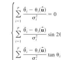
is assumed. The vector of unknowns is now uˆ⫽( A, B, C) and Eq. (2) is used to find it:

冦

_i

冘

_⫽p₁

␪ˆ_{i⫺␪i共uˆ兲}

␴i

2 ⫽0

冘

i⫽1

p

␪ˆ_{i⫺␪i共uˆ兲}

␴i

2 sin 2␪i⫽0

冘

i⫽1

p

␪ˆ_{i⫺␪i共uˆ兲}

␴i

2 tan␪i⫽0

(21)

Once the vector of unknowns is found one can check that A is of the order of 0.01° and all the corrected positions are within an interval of 0.005° from the theoretical ones. All the peaks of the material under investigation are then corrected by

␪corr.⫽␪⫺A⫺B sin 2␪⫺C tan␪ (22)

III. Experimental Procedure

In order to demonstrate the methodology we measured samples of BaTiO3 doped with yttrium and fired under reducing atmo-sphere. The samples were prepared with different stoichiometry of Ba/Ti ratio. Since the yttrium cation can occupy both the barium and the titanium sites, it is expected that for lower titanium chemical potential (barium-rich samples) more yttrium occupies the titanium site, and the lattice expands. A more detailed paper of the specifics of this defect and crystal chemistry is to be published soon.8

The data collection was done with fixed slits using step scan, 0.02° per step, 10 or 20 s/step, as described in Table I. The total time of the measurement is⬃8.7 h.

Our standard material was tungsten (99.9%, Strem Chemicals, Newburyport, MA.), which is cubic with lattice parameter of 3.16524 Å.1

Approximately 1:6 weight tungsten was added, in accordance with the electron density of the two materials. Four peaks of the standard were measured, and typically errors in 2␪of 0.002° or less were obtained after correction.

IV. Results and Discussion

[image:3.612.340.445.59.163.2]

Table II presents the results for one of the samples. As explained above, FWHM and the exponent of the Pearson VII formula (m) are fitted. In cases were split Pearson VII was used, only the pair which generates the larger calculated standard deviation is presented.

Table III presents the lattice parameters of five different samples. Note that the volume difference between barium-rich and

Table I. Measurement Protocol

2_␪range (deg) Peaks covered† Step scan (s/step)

38.4–39.5 1 10

40–40.8 2 10

44.5–46 3, 4 10

55.5–57 5, 6 10

58–59 7 20

65–67 8, 9 10

72.8–73.8 10 20

78–80.4 11, 12 20

83–84.2 13 20

90.3–93.3 14–16 20

116.4–120.7 17–19 20

122–125.3 20–22 20

127–133 23–25 20

138–143 26, 27 20

[image:3.612.327.567.583.736.2]

titanium-rich is significant, taking into account the likelihood standard deviations. Different measurements on samples prepared under the same conditions yielded the same lattice parameters, within the standard deviations.

Table IV presents the results of the analysis of one of the samples, where some of the peaks are omitted. This was done in order to check the sensitivity of the method. It can be seen that less peaks means higher standard deviation, while the lattice parame-ters remain in agreement with those calculated for 23 peaks.

V. Conclusions

(1) MLE was applied for XRD analysis. Under the assumption of a normal distribution of the measured peak position about its true position, the lattice parameters are found by solving the same

equations as in WLS analysis. However, the estimated standard deviations of the lattice parameters are different and can be more accurately determined with the MLE.

(2) Two systems were investigated: cubic and tetragonal. A complete analysis was applied to yttrium-doped BaTiO3 in the tetragonal phase, at room temperature.

(3) A link between the diffractometer’s software output and the standard deviation in the peak position is suggested (Eq. 19). This, along with some restrictions described in Section II (4) is used to evaluate the␴ivalues that are needed for MLE or WLS

analysis.

(4) A protocol for measuring the lattice constants of BaTiO3is described (Table I). It should be possible to compare results from different laboratories if this protocol is to be followed. The authors can also supply a program for the MLE analysis in the form of an MSExcel template on request.

Table II. Results of Sample No. 1.

Peak No. I (counts) 2␪(deg) FWHM (deg) m ⌬2␪(deg) hkl† Corrected␪(deg) Calculated␪(deg)

1 5854 38.936 0.0757 1.035 0.010 111 19.445 19.446

2 2196 40.308 0.0742 1.114 0.010 110W 20.130 20.130

3 2791 44.941 0.0864 0.825 0.010 002 22.445 22.442

4 2561 45.418 0.0895 0.971 0.010 200 22.684 22.690

5 2630 56.023 0.0951 0.817 0.010 112 27.983 27.981

6 5946 56.327 0.0839 1.317 0.010 211 28.135 28.140

7 372 58.308 0.1054 1.054 0.012 200W 29.125 29.125

8 2440 65.793 0.1038 0.919 0.010 202 32.867 32.868

9 971 66.183 0.1010 1.453 0.010 220 33.062 33.060

10 1284 73.242 0.1054 0.863 0.010 211W 36.591 36.591

11 571 78.790 0.1441 0.926 0.015 113 39.365 39.366

12 198 79.497 0.1137 1.150 0.016 311 39.718 39.728

13 1874 83.546 0.1160 0.998 0.010 222 41.743 41.746

14 3446 91.649 0.1223 0.988 0.010 213 45.796 45.796

15 2248 92.095 0.1395 1.213 0.011 312 46.019 46.016

16 2454 92.339 0.1129 1.114 0.010 321 46.141 46.147

17 1070 117.643 0.2250 1.317 0.021 204 58.802 58.806

18 1148 118.860 0.2055 0.838 0.017 402 59.412 59.402

19 1573 119.243 0.1620 1.279 0.014 420 59.603 59.603

20 498 122.554 0.1972 1.118 0.022 214 61.261 61.269

21 861 123.838 0.1844 0.816 0.017 412 61.904 61.897

22 420 124.154 0.1856 2.390 0.023 421 62.056 62.056

23 1086 128.554 0.2289 0.802 0.019 323 64.266 64.267

24 976 129.126 0.2101 0.954 0.019 332 64.552 64.548

25 1664 131.183 0.2392 1.043 0.019 321W 65.591 65.591

26 977 139.568 0.3576 1.133 0.033 224 69.783 69.779

27 2629 141.211 0.3005 1.125 0.022 422 70.607 70.603

†W indicates peaks of the tungsten phase.

Table III. Results of the Analysis of Various Samples

Sample No.

Firing Temperature

(°C) Ba/Ti a (Å) ⌬a (Å) c (Å) ⌬c (Å) V (Å3_{) ⌬V (Å}3₎

1 1350 0.99 3.99377 26⫻10⫺5

4.03554 49⫻10⫺5

64.368 14⫻10⫺3

2 1400 0.99 3.99390 29⫻10⫺5

4.03592 60⫻10⫺5

64.378 16⫻10⫺3

3 1400 1.01 3.99665 39⫻10⫺5

4.03532 76⫻10⫺5

64.457 21⫻10⫺3

4 1400 1.01 3.99581 31⫻10⫺5

4.03716 61⫻10⫺5

64.459 17⫻10⫺3

5 1400 1.01 3.99623 34⫻10⫺5

4.03717 57⫻10⫺5

64.473 17⫻10⫺3

Table IV. Results of the Analysis of Sample No. 1 Taking into Account Different Peaks

Peaks omitted a (Å) ⌬a (Å) c (Å) ⌬c (Å) V (Å3_{) ⌬V (Å}3₎

None 3.99377 26⫻10⫺5

4.03554 49⫻10⫺5

64.368 14⫻10⫺3

3, 4 3.99373 27⫻10⫺5

4.03561 52⫻10⫺5

64.368 15⫻10⫺3

11, 12, 17–19 3.99381 32⫻10⫺5

4.03549 60⫻10⫺5

64.368 18⫻10⫺3

20–24, 26, 27 3.99389 33⫻10⫺5

4.03544 60⫻10⫺5

64.370 17⫻10⫺3

3–6, 17–24, 26, 27 3.99399 51⫻10⫺5

4.03547 88⫻10⫺5

64.374 27⫻10⫺3 1, 3–6, 8, 9, 14–24, 26, 27 3.9942 11⫻10⫺4

4.0355 16⫻10⫺4

[image:4.612.66.571.38.307.2] [image:4.612.64.569.349.433.2] [image:4.612.65.566.665.743.2]

Acknowledgments

We would like to thank A. Hitomi for useful discussions throughout this work. We would also like to thank Y. Huang for her comments on the statistical analysis.

References

1_{H. F. McMurdie, M. C. Morris, E. H. Evans, B. Paretzkin, and W. Wong-Ng,}

“Methods of Producing Standard X-ray Diffraction Powder Patterns,” Powder Diffr.,

1, 40 (1986).

2_{J. Orear, “Notes on Statistics for Physicists, Revised,” Preprint of the Cornel}

Laboratory of Nuclear Studies (unpublished), CLNS 82/511, 1982.

3_{W. K. Meeker and L. A. Escobar, “Maximum Likelihood Method for Fitting}

Parametric Statistical Models”; Ch. 8 in Statistical Methods for Physical Science. Edited by J. L. Stanford and S. B. Varderman. Academic Press, New York 1994.

4_{G. Cassela and L. Berger, “Point Estimation”; Ch. 7 in Statistical Inference.}

Duxbury Press, California, 1990.

5_{H. P. Klug and L. E. Alexander, “Spectrometric Powder Technique”; Ch. 5 in}

X-ray Diffraction Procedures for Polycrystalline and Amorphous Materials, 2nd ed.

Wiley, New York, 1974.

6_{A. J. C. Wilson, “Geiger-Counter X-ray Spectrometer—Influence of Size and}

Absorption Coefficient of Specimen on Position and Shape of Powder Diffraction Maxima,” J. Sci. Instrum., 27, 321 (1950).

7_{J. N. Eastabrook, “Effect of Vertical Divergence in the Displacement and Breadth}

of X-ray Powder Diffraction Lines,” Br. J. Appl. Phys., 3, 349 (1952).

8_{Y. Tsur, A. Hitomi, L. Scrymgeour, and C. A. Randall, “Site Occupancy of}