www.ann-geophys.net/28/753/2010/
© Author(s) 2010. This work is distributed under the Creative Commons Attribution 3.0 License.
Annales
Geophysicae
A new technique for determining orientation and motion of a 2-D,
non-planar magnetopause
A. Blagau1,2, B. Klecker1, G. Paschmann1, S. Haaland3,4, O. Marghitu2,1, and M. Scholer1
1Max-Planck-Institute for extraterrestrial Physics, Garching, Germany 2Institute for Space Sciences, Bucharest, Romania
3Max-Planck Institute for Solar System Research, Katlenburg-Lindau, Germany 4Department of Physics, University of Bergen, Norway
Received: 29 December 2008 – Revised: 4 March 2010 – Accepted: 8 March 2010 – Published: 16 March 2010
Abstract. For a four-point mission like Cluster, the
dif-ferences in position and time when the satellites detect the magnetopause or any other discontinuity, can be used to in-fer the discontinuity local orientation, thickness and motion. This timing technique, commonly assuming a planar geome-try, offers an independent check for various single-spacecraft techniques.
In the present paper we propose an extension of the timing method, capable of determining in a self-consistent way the macroscopic parameters of a two-dimensional, non-planar discontinuity. Such a configuration can be produced by a local bulge or indentation in the magnetopause, or by a large amplitude wave traveling on this surface, and is recognized in Cluster data when the single spacecraft techniques pro-vide different individual normals contained roughly in the same plane. The model we adopted for the magnetopause assumes a layer of constant thickness of either cylindrical or parabolic shape, which has one or two degrees of free-dom for the motion in the plane of the individual normals. The method was further improved by incorporating in a self-consistent way the requirement of minimum magnetic field variance along the magnetopause normal. An additional as-sumption, required in a previously proposed non-planar tech-nique, i.e. that the non-planarity has negligible effects on the minimum variance analysis, is thus avoided.
We applied the method to a magnetopause transition for which the various planar techniques provided inconsistent results. By contrast, the solutions obtained from the dif-ferent implementations of the new 2-D method were con-sistent and stable, indicating a convex shape for the
magne-Correspondence to: A. Blagau ([email protected])
topause. These solutions perform better than the planar so-lutions from the normal magnetic field variance perspective. The magnetopause dynamics and the presence of a non-zero normal magnetic field component in the analyzed event are discussed.
Keywords. Magnetospheric physics (Magnetopause, cusp,
and boundary layers; Instruments and techniques) – Space plasma physics (Discontinuities)
1 Introduction
The macroscopic parameters that characterize a plasma dis-continuity like the terrestrial magnetopause (MP), i.e. the ori-entation, motion, and thickness, are rapidly changing and therefore need to be determined for each particular event.
that region, providing an indication on the plasma regime -whether MHD or kinetic. It also allows us to compute, via Amp`ere’s law, the MP current density, an important parame-ter in the study of plasma instabilities.
The earliest methods for determining the MP orientation use data collected by a single satellite and rely on certain sim-plifying assumptions regarding the discontinuity, like pla-nar geometry, time-statiopla-narity, and variations only along the normal direction for all physical quantities. The first such technique, the minimum variance analysis of the magnetic field (MVAB), developed by Sonnerup and Cahill (1967), is based on O·B=0. Under the mentioned assumptions, this law implies a constant magnetic field component along the discontinuity normal. Consequently, using satellite mea-surements taken during the traversal, the MVAB algorithm identifies the direction along which the magnetic variance is minimized and associates it with the MP normal.
In some cases one can combine results from MVAB and from the so-called deHoffmann-Teller (HT) analysis (e.g., Khrabrov and Sonnerup, 1998a; Paschmann and Sonnerup, 2008), to find also the MP normal velocity. In the HT analy-sis, one searches for a specific reference frame where plasma flow becomes aligned with the magnetic field and thus the motional electric field vanishes. If, based on MP data, the HT frame is identified, one can interpret the measurements as caused by a time-stationary structure moving over the point of observation. Then, by projecting the velocity of the HT frame along the MP normal, one obtains the MP normal ve-locity.
Another single-spacecraft method, the Minimum Faraday Residue (MFR), was developed based on magnetic flux con-servation across the discontinuity (Khrabrov and Sonnerup, 1998b). Here the normal direction and the normal veloc-ity (assumed constant) are found by minimizing the Fara-day residue, i.e. the variance of the tangential electric field component in the discontinuity frame. More recently vari-ous other single-spacecraft techniques were proposed, each based on the conservation of some particular physical quan-tity across the discontinuity. A detailed and unified descrip-tion of these techniques is provided in Sonnerup et al. (2006). For a four-spacecraft mission like Cluster, additional methods for determining the orientation and motion of a dis-continuity are available. These are the timing methods, that use the differences between the positions and times of the MP encounter by the satellites. In general, the timing methods assume also a planar geometry and a steady normal orienta-tion. The first such technique, called time of arrival method, was proposed by Russell et al. (1983), and in addition as-sumes a constant velocity for the discontinuity during the en-tire event. Haaland et al. (2004) introduced a four-point, pla-nar timing technique that assumes a constant thickness for the discontinuity at the scale of the inter-spacecraft separa-tion distance, allowing thus for a variable normal velocity. In that paper, arguments in favor of a constant MP thick-ness as opposed to those in favor of a constant velocity, are
provided. One such argument is that, due to its low mass per unit cross-section, the MP will experience high accelera-tions even for small pressure imbalances, while, on the other hand, the compression is relatively small (of the order of a few percent). Experimental evidence (Dunlop et al., 2001, 2002) supports the idea of a MP undergoing rapid changes in the normal velocity over time-periods comparable to the crossing duration, with relative small variation of its thick-ness. A detailed description of these two approaches, termed Constant Velocity Approach (CVA) and Constant Thickness Approach (CTA), can be found in Haaland et al. (2004).
The problem of determining the macroscopic parame-ters of a more realistic, non-planar discontinuity, when four points of measurements are available, was investigated by Mottez and Chanteur (1994) and Dunlop and Woodward (1998, 1999). These authors developed a method which, in the first stage, applies the MVAB technique on each satel-lite to determine the local discontinuity normal, and after-wards combines these results with the information about the position and time of discontinuity encounter by each satel-lite. For a 3-D discontinuity, with a regular geometry at the scale of the inter-spacecraft separation distance, the two prin-cipal radii of curvature that characterize the surface as well as the velocity and acceleration of the structure can thus be obtained. An important assumption of this method is that the individual normals obtained from a planar technique, i.e. MVAB, are not significantly affected by the local curvature and motion of the non-planar discontinuity during the satel-lite traversal. To our knowledge, the technique has not been quantitatively applied to a four-spacecraft crossing event.
In the present paper we developed a method for determin-ing the macroscopic parameters of a two-dimensional (2-D), non-planar discontinuity, assuming that its thickness can be considered as constant. With the new method the disconti-nuity local orientation, motion, thickness and curvature are obtained simultaneously in a self-consistent way, removing thus the need of an additional assumption, required in the above mentioned non-planar technique, i.e. that of negligi-ble effects due to non-planarity on the results provided by MVAB. In the first instance we extend the planar CTA timing technique, by proposing two simple geometries for the dis-continuity layer, i.e. that of either a cylindrical or a parabolic shape. Later on, the method is improved by incorporating the requirement of minimum magnetic field variance along the instantaneous, local normal, therefore relying simultane-ously on the timing information and on theO·B=0 law. The new method was developed to address the needs described at the beginning of this section, when the MP non-planarity ad-versely influences the values of the macroscopic parameters provided by the planar techniques.
and by the single-spacecraft techniques of MVAB, MFR, and HT, on one hand, and those provided by the 2-D method, on the other hand, will show the advantage of the latter. With the new technique, the MP dynamics and the presence of a non-zero normal magnetic field component in this particular event, will be discussed.
The paper is organized as follows: Sect. 2 introduces the MP crossing from 24 June 2003, providing evidence that the discontinuity has a 2-D, non-planar geometry in this event. Section 3 describes the principles of the new method, with additional details given in Appendix A. Section 4 briefly dis-cusses how the MP moved on 24 June 2003, based on three solutions obtained by applying the 2-D method. An in-depth comparison between one particular 2-D solution and the re-sults provided by the standard, planar methods is presented in Sect. 5, with additional details given in Appendix B. The parameters that characterize all the valid 2-D solutions and the corresponding error analysis are presented in Sect. 6 and in Appendix C. Section 7 provides a discussion of the results obtained with the 2-D method. Section 8 summarizes the re-sults and provides a general perspective, including a list of topics to be addressed in the future.
2 A case of a 2-D, non-planar magnetopause
In this section we present a MP crossing by Cluster on 24 June 2003, to be used as demonstration case for the new 2-D, non-planar technique. We will show that single and multi-satellite planar methods yield inconsistent results, and will provide arguments that the MP has actually a 2-D, non-planar geometry in this case. The direction along which the MP shape does not change, called hereafter the invariant direc-tion, and the timing informadirec-tion, both used as input parame-ters in the new technique, will be determined from the data.
In the present paper we use data from three experiments on-board Cluster. The flux-gate magnetometer (FGM) pro-vides the DC magnetic field vector with an accuracy of about 0.1 nT and a time-resolution of up to 67 samples per second (see Balogh et al., 2001). The Electric Field and Wave (EFW) experiment provides the two electric field components in the spin plane at 25 samples/s in normal mode (see Gustafsson et al., 2001). In favorable conditions the component along the spin axis can be inferred under the assumption thatE·B=0, provided that the magnetic field vector is not too close to the spin-plane. The Cluster Ion Spectrometry (CIS) experiment measures the three-dimensional velocity distribution func-tion of the ions. Based on that, the plasma moments (density, bulk velocity vector, pressure tensor, and heat flux vector) are computed and transmitted to the ground every spacecraft spin period, i.e. every 4 s (see R`eme et al., 2001).
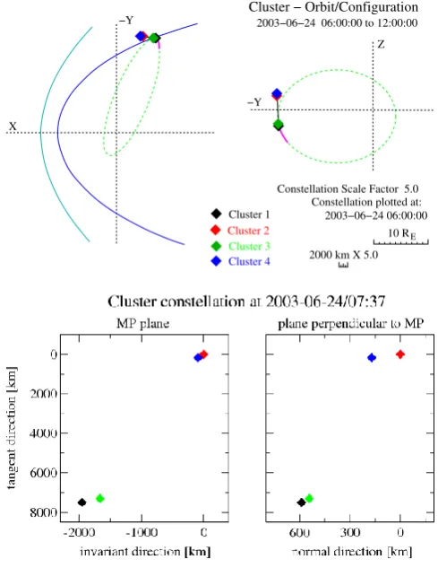
Figure 1 presents the Cluster orbit and configuration for the 24 June 2003 event. The transition that will be analyzed is an inbound crossing and occurred around 07:37:00 UT at the MP dawn flank, near[−7.7,−17.3,−4]Earth radii(RE)
Cluster 1
Cluster 3 Cluster 4
Cluster 2 10 RE
X
−Y
Cluster − Orbit/Configuration
2003−06−24 06:00:00 to 12:00:00
Constellation Scale Factor 5.0 Constellation plotted at:
2003−06−24 06:00:00
2000 km X 5.0 Z
[image:3.595.305.550.63.380.2]−Y
Fig. 1. Upper part: Cluster orbit on 24 June 2003 projected on the
XY and ZY planes of the GSE reference system. The distances between satellites, shown in the mission color code, are increased by a factor of 5. Lower part: Projections of Cluster configuration on the MP plane (left) and on a plane containing the MP normal (right), at the time of the event. More details are given in the text.
in GSE coordinates. In the upper part of the figure, showing the orbit (adapted from Cluster Science Data System web page), a model MP and bow-shock are drawn and the dis-tance between the satellites is scaled by a factor of 5. For this event, the four satellites are traveling in pairs, with Clus-ter 1 (C1) close to C3 (at∼350 km) and C2 close to C4 (at ∼250 km). The distance between the pairs is∼7500 km.
Cluster 2
Cluster 4
Cluster 3
Cluster 1
Cluster 1
Cluster 1
[image:4.595.45.288.65.457.2]Cluster 1
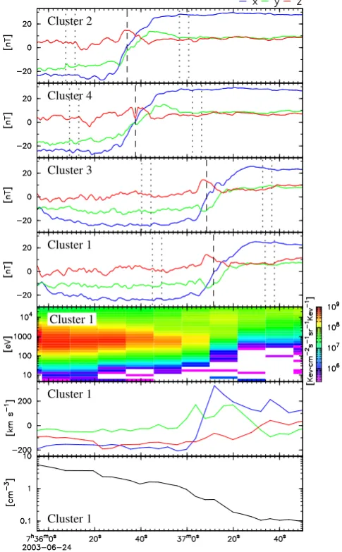
Fig. 2. First four panels: Magnetic field in GSE reference frame measured by Cluster during the MP crossing on 24 June 2003. The panel order, i.e. C2, C4, C3, and C1, corresponds to the sequence of MP encounter. Thex,y, andzcomponents are indicated by the blue, green and red lines respectively. The minimum and maximum length intervals entering the MVAB nested analysis (vertical dot-ted lines) together with their common central time (vertical dashed lines) are shown for each satellite. Last three panels: Ions differ-ential energy spectrogram, bulk velocity components in GSE, and density, as measured by the CIS/Hot Ion Analyser on-board C1.
results obtained with a timing based method. The errors in determining the MP parameters with the new method will be thoroughly analyzed in Appendix C, where it will be shown they stay at an acceptable level. On that point, Figure 2 illustrates one important aspect of the demonstration case, namely a ‘clean’ MP transition at each satellite, with well defined asymptotic levels and a smooth magnetic field tran-sition. This ensures a reliable determination of the timing in-formation (see Subsection 2.3), which indicates clearly
sep-arated satellite transitions, that are at least 2.75 s apart (see Table 2 in that section).
2.1 The results of MVAB. Finding the invariant directionl
In order to reduce the influence of small-scale fluctuations on the MVAB results, we ‘boxcar-averaged’ the initial 0.2 s magnetic data by using a boxcar of 1 s width, followed by a resampling to 0.4 s time resolution. Next, for each satellite, we chose eleven symmetric, nested intervals, centred on a point near the middle of the structure (the central times, the minimum and maximum length of the intervals are presented in Figure 2). For each of these eleven intervals the MVAB was performed, first with the constrainthBi ·n= 0, where
hBiis the average magnetic field (see for example Sonnerup and Scheible, 1998), and, second, without this constraint. In each variant of the method, the average direction, obtained as the component by component average of the eleven normals, was computed.
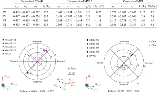
The results are presented in the left and central part of Ta-ble 1. There, for each satellite, the GSE components of the individual normal vectors provided by both MVAB versions are shown, including the ratioλ1/λ2, between the magnetic
field variance along the directions of maximum and interme-diate variance (constrained analysis), and the ratio λ2/λ3,
between the magnetic field variance along the directions of intermediate and minimum variance (unconstrained analy-sis). In addition, for the unconstrained MVAB, the average normal magnetic field componenthBni = hBi ·nis
indi-cated. The ratio of eigenvalues provides a criterion for judg-ing the reliability of the normal determination (see Sonnerup and Scheible, 1998). A rule of thumb requires a value of this ratio&20for the constrained MVAB method and val-ues&10for the unconstrained method. As seen from Table 1, the criterion is easily fulfilled by the constrained MVAB normals, but not by the unconstrained MVAB normals. An-other fact that makes the unconstrained case suspicious is the angle of∼11◦between the C2 and C4 individual normals, which is unreasonably large considering that the satellites are crossing the MP almost simultaneously at a small distance.
Based on these arguments, we shall use only the results provided by the constrained (hBi ·n= 0), MVAB tech-nique. The analysis also indicates a fairly time-stationary MP; for example, in case of C3 the eleven normals corre-sponding to the nested intervals are less than1◦apart from their average.
Figure 3 is a polar plot showing the orientation of the four individual normals obtained from constrained MVAB (the colored squares, symbol MVABC) with respect to their av-erage,hniM V AB, taken as reference direction (the magenta square at the center, symbol MVAB). The vertical line is ori-ented along thehniM V AB×XGSEdirection (roughly along
the south-north direction) and the horizontal line completes the cartesian frame. The components of hniM V AB in the GSE reference frame are indicated at the bottom. Its ori-Fig. 2. First four panels: Magnetic field in GSE reference frame
measured by Cluster during the MP crossing on 24 June 2003. The panel order, i.e. C2, C4, C3, and C1, corresponds to the sequence of MP encounter. The x, y, and z components are indicated by the blue, green and red lines, respectively. The minimum and maximum length intervals entering the MVAB nested analysis (vertical dot-ted lines) together with their common central time (vertical dashed lines) are shown for each satellite. Last three panels: Ions differ-ential energy spectrogram, bulk velocity components in GSE, and density, as measured by the CIS/Hot Ion Analyser on-board C1.
The same sequence is indeed seen in Fig. 2, which presents in the first four panels the magnetic field components mea-sured by each spacecraft in the GSE reference frame. The significance of the various vertical lines indicated in these panels is explained in Sect. 2.1. From the last three pan-els, showing the ion data, i.e. the differential energy spectro-gram, the bulk velocity components in GSE, and the density, measured by the CIS/Hot Ion Analyser on-board C1, one can clearly notice the inbound character of the transition.
The Cluster configuration on 24 June 2003, not being a tetrahedron, may raise concerns about the accuracy of the results obtained with a timing based method. The errors in determining the MP parameters with the new method will be thoroughly analyzed in Appendix C, where it will be shown they stay at an acceptable level. On that point, Fig. 2 illustrates one important aspect of the demonstration case, namely a “clean” MP transition at each satellite, with well defined asymptotic levels and a smooth magnetic field tran-sition. This ensures a reliable determination of the timing information (see Sect. 2.3), which indicates clearly separated satellite transitions, that are at least 2.75 s apart (see Table 2 in that section).
2.1 The results of MVAB – finding the invariant
directionl
In order to reduce the influence of small-scale fluctuations on the MVAB results, we “boxcar-averaged” the initial 0.2 s magnetic data by using a boxcar of 1 s width, followed by a resampling to 0.4 s time resolution. Next, for each satellite, we chose eleven symmetric, nested intervals, centred on a point near the middle of the structure (the central times, the minimum and maximum length of the intervals are presented in Fig. 2). For each of these eleven intervals the MVAB was performed, first with the constraint hBi ·n=0, wherehBi is the average magnetic field (see for example Sonnerup and Scheible, 1998), and, second, without this constraint. In each variant of the method, the average direction, obtained as the component by component average of the eleven normals, was computed.
The results are presented in the left and central part of Ta-ble 1. There, for each satellite, the GSE components of the individual normal vectors provided by both MVAB versions are shown, including the ratioλ1/λ2, between the magnetic field variance along the directions of maximum and interme-diate variance (constrained analysis), and the ratioλ2/λ3, be-tween the magnetic field variance along the directions of in-termediate and minimum variance (unconstrained analysis). In addition, for the unconstrained MVAB, the average normal magnetic field componenthBni = hBi·nis indicated. The ra-tio of eigenvalues provides a criterion for judging the reliabil-ity of the normal determination (see Sonnerup and Scheible, 1998). A rule of thumb requires a value of this ratio&20 for the constrained MVAB method and values&10 for the unconstrained method. As seen from Table 1, the criterion is easily fulfilled by the constrained MVAB normals, but not by the unconstrained MVAB normals. Another fact that makes the unconstrained case suspicious is the angle of∼11◦ be-tween the C2 and C4 individual normals, which is unreason-ably large considering that the satellites are crossing the MP almost simultaneously at a small distance.
Table 1. Results from the constrained (tohBni =0) and unconstrained MVAB averaged over the eleven nested intervals, as well as from the
constrained (tohBni =0) MFR technique. For each satellite, ordered here by the time of MP encounter, the GSE components of the normal
vector, together with the corresponding eigenvalues ratio are presented. In case of the unconstrained MVAB, the resulting average normal magnetic field component is provided as well. The last column shows the angle between the MFR normals and the plane of the normals. More details are provided in the text.
Constrained MVAB Unconstrained MVAB Constrained MFR
nx ny nz λ1/λ2 nx ny nz λ2/λ3 hBni[nT] nx ny nz λ1/λ2 [deg]
C2 0.465 −0.842 −0.272 152 0.467 −0.851 −0.240 3.2 0.22 0.573 −0.807 −0.145 11.7 3.3 C4 0.447 −0.851 −0.274 135 0.458 −0.887 −0.058 2.5 1.34 0.581 −0.807 −0.106 2.9 2.8 C3 0.357 −0.818 −0.451 166 0.331 −0.714 −0.618 7.7 −1.18 0.417 −0.778 −0.470 2.0 4.9 C1 0.333 −0.827 −0.454 138 0.305 −0.716 −0.627 6.2 −1.42 0.361 −0.823 −0.439 2.8 0.4
4
Sunward
Southward Tailward
Northward
Bullseye = [0.403, − 0.839, − 0.365] 8 6 2 MVABC C2
MVABC C3 MVABC C4 MVABC C1
MVAB
XGSM
YGSM
ZGSM
l
BIN T VIN T
BEXT
VEXT k
20nT
[image:5.595.42.551.136.430.2]200km/s
Fig. 3.Polar plot showing the orientation of the four individual normals provided by the constrained MVAB technique (the squares in the mission color code) with respect to their average orientation, taken as reference direction (the central square in magenta). The circles designate directions of equal inclination, in degrees. The individual normals are located roughly in one plane (dashed line), indicating a two-dimensional MP with the invariant direction oriented perpendicular (the unit vectorlin magenta). In the lower left corner, the orientation of GSM coordinate system is shown, as seen when looking against the reference,hniM V ABdirection. The lower right corner presents the tangential components of the magnetic field and velocity flow, as measured by C1, in the regions adjacent to the MP interval: in the magnetosphere (red) and in the magnetosheath (black). The scales of the vectors are also shown. The unit vectork(green) is in the tangent plane and perpendicular to l. More details are provided in the text.
47
Fig. 3. Polar plot showing the orientation of the four individual
normals provided by the constrained MVAB technique (the squares in the mission color code) with respect to their average orientation, taken as reference direction (the central square in magenta). The circles designate directions of equal inclination, in degrees. The dividual normals are located roughly in one plane (dashed line), in-dicating a two-dimensional MP with the invariant direction oriented perpendicular (the unit vectorlin magenta). In the lower left corner, the orientation of GSM coordinate system is shown, as seen when looking against the reference,hniMVABdirection. The lower right corner presents the tangential components of the magnetic field and velocity flow, as measured by C1, in the regions adjacent to the MP interval: in the magnetosphere (red) and in the magnetosheath (black). The scales of the vectors are also shown. The unit vectork
(green) is in the tangent plane and perpendicular tol. More details are provided in the text.
example, in case of C3 the eleven normals corresponding to the nested intervals are less than 1◦apart from their average. Figure 3 is a polar plot showing the orientation of the four individual normals obtained from constrained MVAB (the colored squares, symbol MVABC) with respect to their
av-MFRC C1 MFRC C2 MFRC C3 MFRC C4 MVAB
CTA CVA
30
Southward Tailward
Northward
10 20 Sunward
Bullseye = [0.403, − 0.839, − 0.365]
XGSM
YGSM
[image:5.595.303.543.262.424.2]ZGSM
Fig. 4.Polar plot having the same reference direction as Figure 3 for an increased angular range. It shows the orientation of the individual normals provided by the constrained MFR technique (rhombs), the CVA (red open circle), and CTA (golden open circle) normals, provided by the planar timing analysis. Theplane of the normals(see text) is indicated with a dashed line.
48
Fig. 4. Polar plot having the same reference direction as Fig. 3 for
an increased angular range. It shows the orientation of the individ-ual normals provided by the constrained MFR technique (rhombs), the CVA (red open circle), and CTA (golden open circle) normals, provided by the planar timing analysis. The plane of the normals (see text) is indicated with a dashed line.
erage, hniMVAB, taken as reference direction (the magenta square at the center, symbol MVAB). The vertical line is ori-ented along thehniMVAB×XGSEdirection (roughly along the south-north direction) and the horizontal line completes the cartesian frame. The components ofhniMVABin the GSE ref-erence frame are indicated at the bottom. Its orientation with respect to the GSM reference frame can be judged by looking at the unit vectors on the bottom left part of the figure. The circles designate directions of equal inclination with respect tohniMVAB, in degrees. For each individual normal, an error bar is drawn, indicating the orientation uncertainty due to the statistical errors (see Sonnerup and Scheible, 1998).
intersection with the closest (in the least square sense) plane situated between the normals. All four MVAB normals lie within 0.7◦of it. Between the normals detected by C2 and C1 (i.e. the first and the last satellite crossing the MP) the difference in orientation is about 12.5◦. Considering that the individual, constrained MVAB normals appear to be very re-liable, we interpret the results as the effect of Cluster en-countering a 2-D, non-planar MP. The plane indicated by the dashed line will be called hereafter the plane of the normals. The invariant direction, used as input parameter in the new 2-D technique, is perpendicular to that plane and indicated by the unit vectorl. Its components in the GSE reference frame are[−0.748,−0.532,0.398].
The individual normals are grouped two by two (C1 with C3 and C2 with C4), a consequence of the Cluster satellites crossing the MP in pairs. Due to this particular formation, one cannot rule out a priori the possibility of a planar MP that changed its orientation between the crossing of the two pairs. However, one can consider such a situation a limiting case, when the 2-D MP surface has a very large radius of curvature. It will become clear in Sect. 3 that solutions of this kind are not excluded by the new method. For the 24 June 2003 event, we shall come back to this aspect in Sect. 5, where the results obtained by applying the new 2-D method are discussed.
In the lower right corner of Fig. 3 we plotted the tan-gential components of the magnetic field and flow velocity vectors measured by C1 in the regions adjacent to the MP, i.e. the magnetosphere interior (in red, the vectorsBINTand VINT) and the magnetosheath (in black, the vectorsBEXT andVEXT). Each vector is an average over 5 data points, corresponding to the time intervals [07:37:36–07:37:52], and [07:36:31–07:36:47] respectively. The angle between the two flow directions is∼172◦ and the magnetic field shear angle is∼150◦.
At the bottom of Fig. 1, showing the Cluster constella-tion at the time of the event, thexaxis is oriented alonglin the left projection, while in the right projection it lies along hniMVAB. Theyaxis, the same in both pictures, is oriented alonghniMVAB×l.
Additional arguments in favor of a 2-D geometry for the MP on 24 June 2003 will be provided in Sects. 2.2 and 2.4, where the results obtained by applying the planar MFR and timing analysis methods will be shown.
2.2 The results of MFR
For carrying out the MFR analysis we need both magnetic field and high-resolution electric field data1. Unfortunately, during some parts of the crossings, the magnetic field vector was close to the spacecraft spin plane. Because this leads to 1The relatively fast transitions seen by Cluster on 24 June 2003,
results in a number of data points too low to apply MFR to the 4 s, spin-resolution convection electric field,E= −v×B, derived from the plasma velocityvmeasured by CIS.
high uncertainties when constructing the third, spin-aligned electric field component, for those parts of the MP transition the data cannot be used. However, for all the Cluster satel-lites, the interval used in the MFR analysis is wide enough to include the MP central portion (i.e. corresponding to the central interval[Tci−τi, Tci+τi]defined in Sect. 2.3).
Like in the MVAB case, to reduce the influence of small-scale fluctuations on the MFR results, we “boxcar-averaged” the high-resolution data using a 2 s boxcar window, followed by a resampling to 0.5 s time-resolution. Each individual MFR normal was obtained by constraining the average nor-mal magnetic field component to zero, i.e.hBi ·n=0. The results are presented in the right part of Table 1. For each satellite, the GSE components of the normal vectors, together with the eigenvalues ratioλ1/λ2 are shown. The last col-umn presents the angle, made by the individual MFR nor-mals with respect to the plane of the nornor-mals, determined in Sect. 2.1.
As Table 1 shows, the MFR normals are not so well de-fined, except, perhaps, the C2 normal, with a ratio λ1/λ2 around 11.7. One possible explanation could be that, due to the already mentioned data gaps, the intervals used in the MFR analysis do not include the whole MP transition. In-deed, in case of C2, approx. 93.7% of the magnetic field ro-tation occurs during the MFR interval (the largest fractional change) whereas for C3, whenλ1/λ2'2, the MFR inter-val covers only 76.2% of the total magnetic field change (the smallest fractional change).
Figure 4 is a polar plot with the same reference direction as Fig. 3, i.e.hniMVAB(central magenta square), but has an increased angular range. The plane of the normals, obtained in Sect. 2.1, is indicated by the dashed line. The individual MFR normals are shown as colored rhombs (symbol MFRC), together with their corresponding statistical error bars.
The orientation of the individual MFR normals obtained in the analysis are certainly corrupted by the MP non-planarity. However, for an ideal 2-D discontinuity, the normals pro-vided by the planar MFR technique would be contained in one plane, the same that contains also the individual MVAB normals. It is remarkable that in our case, in spite of the men-tioned problems with the data, the constrained MFR normals lie very close, basically within the statistical errors, to the plane of the normals identified in Sect. 2.1 (see parameter in the Table 1). In fact, if we proceed as described at the end of Sect. 2.1 and compute the invariant direction based entirely on the individual MFR normals, we obtain a direc-tion only 3◦away off the invariant direction computed there. Thus, the MFR results are consistent with the earlier conclu-sion of a 2-D, non-planar MP.
2.3 Extracting the timing information
100 110 120 130 140 150 160 170
seconds since 2003−06−24/07:35:00
−30 −20 −10 0 10 20 30
B components [nT]
fitted points MP edges Tc= 132.75
[image:7.595.47.288.63.234.2]τ= 9.29
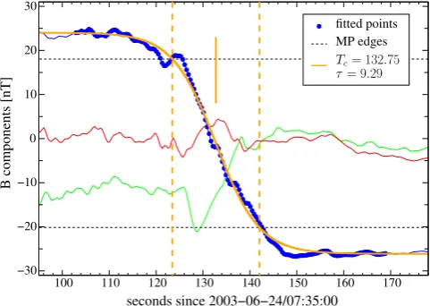
Fig. 5.C1 magnetic field components along the directions of minimum magnetic field variance (red trace), of maximum magnetic field variance (blue trace) and alonghBi(green trace). The timing information, shown in the legend box, is obtained by fitting the points (in blue) corresponding to the maximum variance component with a hyperbolic tangent function, shown in orange. More details are provided in the text.
[image:7.595.315.542.144.236.2]49
Fig. 5. C1 magnetic field components along the directions of
min-imum magnetic field variance (red trace), of maxmin-imum magnetic field variance (blue trace) and alonghBi(green trace). The tim-ing information, shown in the legend box, is obtained by fitttim-ing the points (in blue) corresponding to the maximum variance component with a hyperbolic tangent function, shown in orange. More details are provided in the text.
each satellite was transformed into the local MP frame pro-vided by the constrained MVAB analysis, having the axes along the directions providing the maximum magnetic vari-ance, the minimum magnetic variance and along the direc-tion ofhBi. Then, the maximum magnetic variance compo-nent was fitted with a hyperbolic tangent function
B(t )=Bm− 1
21Btanh
t−T
c τ
in order to determine the crossing time that characterizes the MP transition in the global sense. HereBmis the zero level of the tanh function,1Bis the total magnetic jump between the magnetosheath and magnetopause asymptotic levels,Tc represents the central time andτ designates the profile half-width. Note that, because of a non-planar MP, we expect that the direction providing the minimum magnetic field variance will be different from one satellite to another and therefore each fit will be performed in a slightly different reference frame.
Next, a definition for the MP extent as the central re-gion where the fit changes from Bm−121Btanh(−1) to Bm−121Btanh(1)magnetic levels was adopted. This cor-responds to a fraction of∼0.762 of the total magnetic jump 1B. According to this definition, the satellite encounters the MP leading edge atTc−τand the MP trailing edge atTc+τ. These two instants of time will be used directly in the method (not the central crossing timeTc, as in Haaland et al. 2004).
As an illustration of the procedure described above, Fig. 5 presents the C1 magnetic field components in the reference frame related to the corresponding MVAB normal. The magnetic field components along the direction providing the
Table 2. Satellite relative positions and timing for the analyzed event. For each satellite the components along thel,hniMVAB, and
tdirections (see the text) are provided, together with the MP central crossing timeTc, and crossing durationτ. The C2 position is taken
as origin of the reference frame and theTcquantities are computed
with respect to the C2 central crossing time.
position[km] timing[s]
Rl Rn Rt Tc τ
C2 0.0 0.0 0.0 0.0 6.44
C4 −90.6 170.9 167.6 2.75 7.27
C3 −1664.9 541.9 7306.5 34.87 8.91
C1 −1954.5 588.1 7506.0 37.81 9.29
maximum magnetic field variance, the minimum magnetic field variance and along the direction ofhBiare shown by blue, red and green lines respectively. The points included in the fit are shown in blue. The parametersTc(indicated by the vertical yellow segment) andτ(the half-distance between the vertical yellow dashed lines) determined in the analysis are provided in the insert. The horizontal dashed lines represent the magnetic field levels associated with the MP edges.
Table 2 presents the satellites’ relative positions and the timing information for the 24 June 2004 event. The quanti-tiesRl,Rn,Rt, are the separation distances along the invari-ant directionl, alonghniMVAB, and along t= hniMVAB×l, respectively. We choose as reference the position of C2, i.e. the first satellite detecting the MP. The central crossing times Tc, computed with respect to the time when C2 detects the MP center, and the crossing durationsτ are shown. From Table 2 one can observe that the satellites MP transitions are well separated, the minimum separation being 2.75 s.
2.4 The results from planar timing analysis
When carrying out the CVA and CTA timing analysis (Haa-land et al., 2004), in order to stay fully consistent with the planar assumption, where a single normal direction charac-terizes the event, the timing information was extracted from fits similar to that presented in Fig. 5 but on magnetic traces in a common reference frame, related to thehniMVAB direc-tion2.
In Fig. 4 the CVA and CTA normals are indicated with red and golden open circles respectively. Their orientation is well apart from thehniMVABdirection, i.e.∼32◦and∼38◦ for the CTA and the CVA normals, respectively. Consider-ing the regular magnetic profiles seen by all satellites and the good quality of the fits, resulting in a trustworthy timing 2In our particular case this aspect has practically no influence:
information, this discrepancy is very significant, suggesting again a non-planar geometry for the MP.
To save the planar assumption, one could argue that, per-haps, neither the constant thickness nor the constant velocity assumptions are valid for this event but, instead, there is a variable normal velocity and the MP has different thickness at different points on its surface. We investigated this pos-sibility by imposing different orientations for a planar layer, around the direction of hniMVAB. Then, the central cross-ing times and the relative positions of the satellites along the imposed normal allow us to determine the MP normal veloc-ity evolution3. By proceeding in this way, and imposing for examplehniMVABas normal direction, one obtains unreason-ably large variations in the MP thickness from one satellite to another. For example, between C3 and C1, separated by only 202 km in the MP plane, a MP thickness variation of 183 km, from 254 km to 437 km, was obtained. A similar behavior was noticed for other directions close to thehniMVAB.
An interesting observation related to Fig. 4 is the follow-ing: when the MVAB technique, which assumes a planar ge-ometry, is applied on a 2-D discontinuity, the normal orienta-tion will be affected by the non-planarity. However, the infor-mation about the 2-D symmetry contained in the actual mag-netic measurements (ideally, the measurements will not vary along the invariant direction) is reflected in the result, and the normal will lie in the plane perpendicular to the invari-ant direction. The same consideration applies to the planar MFR technique as well. By contrast, because the techniques employed in this subsection rely solely on the satellites po-sition and on the timing information, a 2-D MP investigated with the standard CVA or CTA will not produce, in general, normals in the plane perpendicular tol.
3 Presentation of the new method
The new method assumes that the MP can be locally mod-elled as a layer of constant thickness that has either a parabolic or a cylindrical shape, that does not change along the direction perpendicular to the plane of the normals (the invariant direction). In the plane of the normals we allow for the layer to have either a unidirectional movement or in-dependent motions along two mutually perpendicular direc-tions. Any motion along the third, invariant direction has no meaning because it causes no change. Note that this model can describe two main features of the non-planar MP: its inward-outward motion and, by allowing for a second degree of freedom, the large-scale waves that often travel along its surface.
There are actually two techniques that we developed for determining the crossing parameters of a 2-D, non-planar discontinuity. The first is based, apart from the knowledge of invariant direction, solely on the timing information, thus 3A second degree polynomial has been used to describe the MP
normal velocity time-dependence.
being a generalization of the planar CTA technique. The sec-ond technique uses simultaneously the timing information and theO·B=0 conservation law, providing solutions that comply with the requirement of minimum normal magnetic field variance. The two techniques, which we will refer to as the straight timing analysis and the combined timing – MVAB analysis, are briefly described in Sect. 3.1 and Sect. 3.2, re-spectively. Additional details are given in Appendix A.
3.1 Straight timing analysis
Let us suppose that the necessary input parameters, i.e. the invariant direction and the timing information, were ex-tracted from the data, as shown in Sect. 2.3 for the 24 June 2003 event. Then, mathematically, in each implementation of the model (parabolic or cylindrical geometry, one or two degrees of freedom for the MP movement), a system of eight equations can be established, i.e. two equations for each satellite. This corresponds to the conditions that, during its motion, the leading and trailing edges of a 2-D MP oriented along the invariant direction encounters the satellites’ po-sitions according to the timing information. Note that the method uses the times when the satellites detect the MP lead-ing and traillead-ing edges, and not the time when the MP center is detected, contrary to the planar CTA and CVA methods.
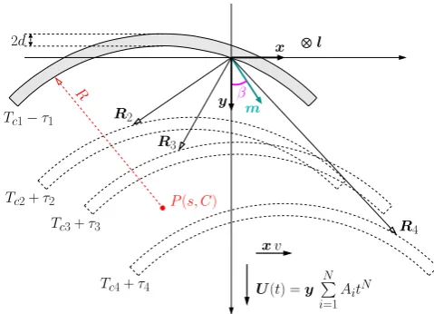
Figures 6 and 7 schematically show cross-sections of a parabolic, respectively cylindrical, MP at successive times (more explanations related to the figures are given in Ap-pendix A). The invariant directionlpoints into the page. The unknowns to be found from the above mentioned system of eight equations are:
– the spatial scale of the structure, given by the quadratic
coefficient of the parabola describing the MP profile, in the parabolic case, or by the MP inner radius of curva-ture, in the cylindrical case;
– the MP thickness;
– the angle in the plane of the normals specifying the
di-rection of primary MP motion (see below);
– the initial position of the structure, given by two
coor-dinates in the plane of the normals, specifying the MP leading edge apex position, in the parabolic case, or the MP center of curvature, in the cylindrical case;
– three coefficients describing the velocity-time
depen-dence, assumed to be polynomial.
x
y
l
m
β Tc1−τ1
Tc2+τ2
Tc3+τ3
Tc4+τ4
2d
P(s, C)
R2
R3
R4 xv
U(t) =y N
P
[image:9.595.306.546.62.235.2]i=1 AitN
Fig. 6.MP as a parabolic layer, in cross-sections at successive moments. The unit vectorl, indicating the invariant direction, points into the paper. The Cluster satellites are located atRi, i= 1...4, withR1≡0. At the initial time,Tc1−τ1, the parabola describing the MP leading edge has the apex atP(s, C), and encounters the first satellite at the origin; at the other three times shown, atTci+τi, i= 2...4, the MP trailing edge is detected by the second, third and fourth satellite, respectively. According to the model, the MP primary movement, with a polynomial time dependence for velocity, takes place alongy, parallel to the parabola’s axis. The secondary movement, allowed in one variant of the model, occurs with constant velocity in the perpendicular direction. Details about the quantities shown in this figure are discussed in Appendix A.
50
Fig. 6. MP as a parabolic layer, in cross-sections at successive
mo-ments. The unit vectorl, indicating the invariant direction, points into the paper. The Cluster satellites are located atRi, i=1...4, withR1≡0. At the initial time,Tc1−τ1, the parabola
describ-ing the MP leaddescrib-ing edge has the apex atP (s,C), and encounters the first satellite at the origin; at the other three times shown, at
Tci+τi, i=2...4, the MP trailing edge is detected by the second,
third and fourth satellite, respectively. According to the model, the MP primary movement, with a polynomial time dependence for ve-locity, takes place alongy, parallel to the parabola’s axis. The sec-ondary movement, allowed in one variant of the model, occurs with constant velocity in the perpendicular direction. Details about the quantities shown in this figure are discussed in Appendix A.
characterize the structure’s velocity, acceleration and change in the acceleration, respectively.
3.2 Combined timing – MVAB analysis
The straight timing analysis presented in the previous subsec-tion can be improved if one takes advantage of the fact that the primary direction of MP movement is fully described by one parameter, i.e. an angle in the plane of the normals.
Based on that, one can impose different values for this pa-rameter, and solve the system of eight equations from the previous subsection with this condition. For each solution that is found, corresponding to one angle, the magnetic field variance along the instantaneous, i.e. geometrical, MP nor-mal at each satellite can be computed.
σi2= 1 Mi
Mi
X
m=1
B(m)i − hBii·n(m)2D,i
2
i=1...4 (1)
Here B(m)i , m=1...Mi, represent the magnetic measure-ments taken by satellitei, andn(m)2D,i designates the 2-D, in-stantaneous geometrical normal at the same satellite. The superscriptmindicates that these normals are changing in time and therefore their orientation at the time when theB(m) measurement is taken will be considered in Eq. (1).
x
y Tc1−τ1
Tc2+τ2
Tc3+τ3
Tc4+τ4
P(s, C)
2d
R
R2
R3
R4 m
l
β
U(t) =y N
P
[image:9.595.46.286.66.232.2]i=1 AitN xv
Fig. 7.Figure similar to Figure 6 but corresponding to a cylindrical MP layer. Now the coordinates(s, C) indicate the MP center of curvaturePat the initial timeTc1−τ1. Details about the quantities shown in this
figure are discussed in Appendix A.
51
Fig. 7. Figure similar to Fig. 6 but corresponding to a cylindrical
MP layer. Now the coordinates(s,C)indicate the MP center of curvatureP at the initial timeTc1−τ1. Details about the quantities
shown in this figure are discussed in Appendix A.
If the angle defining the direction of MP movement is in-creased stepwise, within the range[−π,π], one can select that direction of MP movement for which the global nor-mal magnetic field variance is minimum. Here by “global”, a weighted average over the four satellites is meant, i.e. σglobal2 =P4
i=1piσi2. Details about how to define the cor-responding weighting factorspi are provided in Appendix A (see Eq. A5), the underlying argument being the following: if the magnetic field measured at one satellite is, by what-ever reason, more perturbed than at the other, i.e. if it implies higher magnetic field fluctuations, then its contribution to the global magnetic field variance is reduced by the weighting factor.
The solution obtained in this way has two advantages: first, it combines in a self-consistent way the timing infor-mation with the requirements ofO·B=0. Second, because the angle specifying the direction of MP movement is now set from outside, four coefficients, instead of three, are avail-able to describe the MP velocity-time dependence, providing an improved description of the MP motion.
4 Solutions provided by the 2-D, non-planar method
A
C
B
D
−8000 −6000 −4000 −2000 −8000 −6000 −4000 −2000
0 2000 4000
−8000 −6000 −4000 −2000 0 2000 4000
0 2000 4000 6000 8000 0 2000 4000
0 2000 4000 6000 8000
−8000 0 2000 4000
nMVAB n2D leading edge
2D
Cluster 1
Cluster 4
secondary direction [km]
primary direction [km]
Cluster 3 Cluster 2
n trailing edge XGSM
ZGSM
YGSM
x y
[image:10.595.50.288.61.367.2]hniM V AB hniext
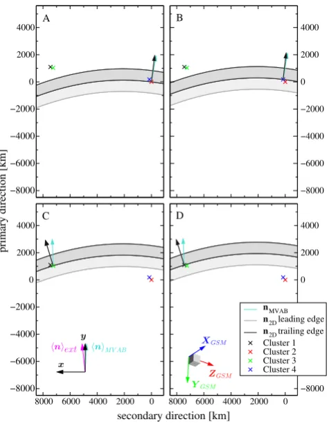
Fig. 8.The 2-D, non-planar MP motion in the plane perpendicular to the invariant direction, according to the P1 OpTAsolution. For a description of this picture see the text.
52
Fig. 8. The 2-D, non-planar MP motion in the plane perpendicular
to the invariant direction, according to theP1 OpTAsolution. For a description of this picture see the text.
MVAB technique). For the cylindrical MP having 2 degrees of freedom, two solutions have been found with the com-bined timing-MVAB technique; they will be differentiated by the suffix “A” and “B”, respectively.
This section presents three exemplary 2-D, non-planar so-lutions, one based on the parabolic model, i.e. P1 OpTA
shown in Fig. 8, and two on the cylindrical model, i.e.
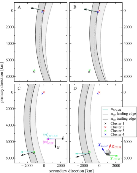
C2 OpTA AandC2 OpTA Bshown in Fig. 9 and Fig. 10, respectively. For a detailed presentation of all 2-D solutions, the reader is referred to Blagau (2007).
In Figs. 8, 9, and 10, the spacecraft positions are indicated by crosses, colored according to the mission convention. The panels A, B, C, and D are associated with the satellite C2, C4, C3, and C1 respectively, and present the MP cross-sections in the plane perpendicular to the invariant directionlat two moments: when the corresponding satellite enters the layer (i.e. atTci−τi, i=1...4, in light gray) and when it leaves the layer (i.e. atTci+τi, in darker gray). The MP external geometrical normals4,n2D, at the satellite position for these 4Here by “external geometrical” we mean pointing into the
op-posite direction of the center of curvature, not the direction outward from the magnetosphere. Whether the two directions are parallel or anti-parallel depends on the center of curvature location, i.e.
ei-0
2000
4000
6000
8000
0
2000
4000
6000
8000
− 4000 − 2000 0 0
2000
4000
6000
8000
− 4000 − 2000 0
0
2000
4000
6000
8000 6000
nMVAB n2D leading edge n2D trailing edge
Cluster 1 Cluster 2 Cluster 3 Cluster 4
secondary direction [km]
primary direction [km]
A
C
B
D
XGSM
ZGSM
YGSM x
y hniM V AB
[image:10.595.308.547.62.361.2]hniext
Fig. 9.The 2-D, non-planar MP motion in the plane perpendicular to the invariant direction, according to the C2 OpTA Asolution. For a description of this picture see the text.
53
Fig. 9. The 2-D, non-planar MP motion in the plane perpendicular
to the invariant direction, according to theC2 OpTA A solution. For a description of this picture see the text.
two moments are shown, together with the individual normal obtained from the planar, nested MVAB technique (in cyan; actually the projection of this normal on the plane perpendic-ular to the invariant direction is shown).
The primary movement takes place alongy, i.e. along the vertical. In the last two solutions, see Figs. 9 and 10, the MP has also a secondary motion, with constant velocity, alongx. In panel (c), besides they andx axes, two other directions are shown. In light blue is the average of the planar, individ-ual normals obtained in the nested MVAB analysis,hniMVAB, chosen also as reference direction in Figs. 3 and 4 from Sect. 2. For the second direction, one first computes for each satellite the individual n2Dave normal, i.e. the average (over the crossing duration) external geometrical normal based on the 2-D solution. The unit vectorhniext, shown in magenta, is along the vectorial mean of the four n2Dave normals. In panel (d), the orientation of XGSM, YGSM and ZGSM, i.e. the unit vectors defining the GSM reference frame, as seen by looking against the invariant directionl(pointing into the page) are indicated.
0
2000
4000
6000
8000
0
2000
4000
6000
8000
− 2000 0 2000 0
2000
4000
6000
8000
− 2000 0 2000 0
2000
4000
6000
8000 nMVAB n2D leading edge n2D trailing edge
Cluster 1 Cluster 2 Cluster 3 Cluster 4
secondary direction [km]
primary direction [km]
A
D B
C
XGSM Z GSM
YGSM x
y hniM V AB
[image:11.595.48.287.61.363.2]hniext
Fig. 10.The 2-D, non-planar MP motion in the plane perpendicular to the invariant direction, according to the C2 OpTA Bsolution. For a description of this picture see the text.
54
Fig. 10. The 2-D, non-planar MP motion in the plane perpendicular
to the invariant direction, according to theC2 OpTA Bsolution. For a description of this picture see the text.
Since, by definition,hniextis oriented into the opposite di-rection of the center of curvature, the in-bound character of the transition (see the beginning of Sect. 2) implies a con-vex shape for the MP depicted in Figs. 8, 9 and 10 (the same result has actually been obtained from all acceptable 2-D so-lutions corresponding to the 24 June 2003 event; see Bla-gau, 2007). The solutionP1 OpTAfrom Fig. 8 is consistent with a local, stationary bulge on the MP surface, modelled by a parabolic layer moving (outward) exclusively along the ydirection. The other two cases, shown here in Fig. 9 and Fig. 10, indicate a traveling wave on the MP surface: the general outward motion occurs with constant velocity along the x direction, while a more complicated, back and forth movement takes place along theydirection.5
The solution C2 OpTA A from Fig. 9 implies a re-encounter of the MP by the first pair of satellites (C2 and C4) at the end of the event, i.e. around the time when the second 5Note that for these two solutions, the primary directionyis not
oriented close to the MP normal but it is roughly perpendicular to it, i.e. opposite of the situation depicted in Fig. 7. This is because we did not impose any restriction of this kind in the model; the orientation ofxandyaxes is obtained exclusively by solving the conditions of MP encounter.
pair of satellites (C3 and C1) finish their transitions. The re-turn is not seen in the data and strictly speaking means a dis-agreement with the physical situation. This aspect could be reconciled if one limits in an appropriate way the solution’s range of validity, like has been done in Fig. 9, where the up-per part of the MP was not sketched. No such limitation was needed for theP1 OpTAandC2 OpTA Bsolutions.
It is worth mentioning that the C2 OpTA A solution, shown in Fig. 9, and theC2 TAsolution, not shown here, are practically identical. This is remarkable, meaning that the method based solely on the timing information already provides a result optimized with respect to theO·B=0 con-servation law.
The parameters that characterize all the valid 2-D solu-tions corresponding to 24 June 2003 event will be presented in Sect. 6, when also the normal magnetic field variance and the average normal magnetic field quantities implied by each solution are shown. It will be clear that, in spite of the appar-ent diversity, the MP transition parameters (oriappar-entation, nor-mal velocity, thickness and curvature) obtained by the vari-ous implementations are actually not very different.
5 Detailed presentation of one 2-D solution
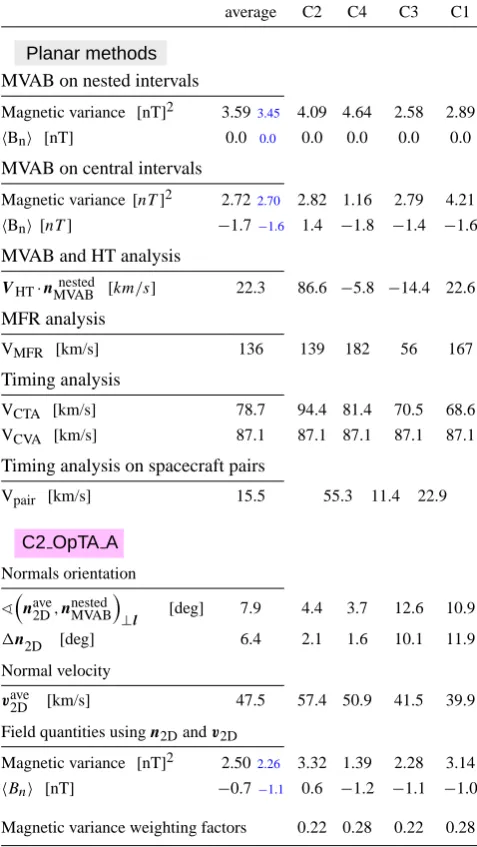
In this section, the solutionC2 OpTA Afrom Fig. 9 (i.e. the first solution found with the combined timing-MVAB tech-nique for a cylindrical MP having two degrees of freedom) will be discussed in detail and compared with the results pro-vided by the planar methods like MVAB, MFR, timing anal-ysis, and HT analysis. Table 3 summarizes this comparison both in terms of individual quantities, i.e. corresponding to each satellite, as well as in terms of the average, or “global” ones. Below a brief description of the parameters shown in this table is given.
The Planar methods part of Table 3 presents first the results of the constrained MVAB analysis on eleven nested intervals (see Sect. 2.1) in terms of normal magnetic field variance and average normal magnetic field componenthBni. The next two lines show similar quantities obtained by ap-plying a constrained MVAB analysis on the central intervals [Tci−τi, Tci+τi]. Here the constraint l·n=0 has been used, thus eliminating in the analysis the influence of mag-netic fluctuations perpendicular to the plane of the normals, in accordance with the 2-D geometry assumption for the MP. Further on, the normal MP velocity is presented, as deter-mined by combining the nested MVAB normals with the HT analysis (see Sect. 5.3), by applying the MFR technique (see Sect. 2.2), and by applying the two variants of the planar tim-ing analysis, i.e. CTA and CVA (see Sect. 2.4).
Table 3. Comparison between theC2 OpTA Asolution and the planar results provided by MVAB, HT, MFR, and timing analysis techniques. Quantities corresponding to each satellite as well as average or global ones are shown. With smaller blue numbers, the global values of normal magnetic field variance and ofhBnibased
only on data from C1, C3 and C4 are indicated. More explanations are provided in the text.
average C2 C4 C3 C1
Planar methods
MVAB on nested intervals
Magnetic variance [nT]2 3.593.45 4.09 4.64 2.58 2.89
hBni [nT] 0.0 0.0 0.0 0.0 0.0 0.0
MVAB on central intervals
Magnetic variance[nT]2 2.722.70 2.82 1.16 2.79 4.21
hBni [nT] −1.7−1.6 1.4 −1.8 −1.4 −1.6
MVAB and HT analysis
VHT·nMVABnested [km/s] 22.3 86.6 −5.8 −14.4 22.6
MFR analysis
VMFR [km/s] 136 139 182 56 167
Timing analysis
VCTA [km/s] 78.7 94.4 81.4 70.5 68.6
VCVA [km/s] 87.1 87.1 87.1 87.1 87.1
Timing analysis on spacecraft pairs
Vpair [km/s] 15.5 55.3 11.4 22.9
C2 OpTA A
Normals orientation
^nave 2D,nnestedMVAB
⊥l [deg] 7.9 4.4 3.7 12.6 10.9
1n
2D [deg] 6.4 2.1 1.6 10.1 11.9
Normal velocity
vave
2D [km/s] 47.5 57.4 50.9 41.5 39.9
Field quantities usingn2Dandv2D
Magnetic variance [nT]2 2.502.26 3.32 1.39 2.28 3.14
hBni [nT] −0.7−1.1 0.6 −1.2 −1.1 −1.0
Magnetic variance weighting factors 0.22 0.28 0.22 0.28
the average of the coresponding MVAB normals and there-fore the Vpairquantities were computed based on the satel-lites separation along that direction and on the difference Tc,i+1−Tc,i. The MP global velocity, presented in the first column, is a weighted average which takes into account that eachVpairis valid for a different time length.
In theC2 OpTA Apart of Table 3, all quantities refer to the central intervals. The first line presents the angle between then2Daveand the individual MVAB normals, projected on the
plane perpendicular to the invariant directionl, and reflects the difference in normal prediction by the two methods. The second line shows the change in orientation of the instanta-neous geometrical normals,n2D, during the crossing interval, measuring how the MP movement and curvature influence the normal detected by the satellites. The average (over the crossing duration) MP normal velocity,vave2D, is shown on the following line. Next, the normal magnetic field variance and the values forhBniare presented.
The weighting factors, used to compute the global value of the normal magnetic field variance, are shown on the last line. They were derived based on the arguments presented in Appendix A (see the discussions related to Eq. A5).
5.1 The investigation of normal magnetic field variance
When judging whether the planar or the 2-D method pro-vides solutions that comply better with the requirement of minimum normal magnetic field variance, one has to take into account that each technique uses different data inter-vals: the planar MVAB is based on data intervals large enough to include the whole magnetic field rotation seen at the MP, whereas in the 2-D method only the central intervals, [Tci−τi, Tci+τi], are used, in accordance with the system of conditions describing the satellites encounter with the MP edges. Therefore, it is instructive to investigate how the solu-tions provided by the two techniques behave starting from the central intervals up to the largest intervals used in the nested MVAB analysis (see Sect. 2.1).
Such an investigation has been carried out in Appendix B. There, using intervals centred onTci that progressively in-crease in size, we analyzed the evolution of the normal mag-netic field variance and of the average normal magmag-netic field componenthBni, based on three sets of normals: the individ-ual, planar normals obtained from the nested MVAB analy-sis, the 2-D, instantaneous, geometrical normals correspond-ing to theC2 OpTA Asolution and the normals provided by a constrained, tol·n=0, MVAB analysis performed for that particular interval. Note that the latter normals, called here and in Appendix B the planar, interval-specific MVAB nor-mals, are changing with the interval of analysis according to the MVAB theory.
The analysis shows that, even for intervals well beyond the validity range of the 2-D solution, i.e.[Tci−τi, Tci+τi], the global magnetic field variance based on the 2-D, geometri-cal normals is smaller than the same quantity based on the planar, interval-specific MVAB normals (which is, evidently, smaller than that based on the normals provided by the nested MVAB analysis). Therefore one can definitely say that, for the above mentioned intervals, the 2-D solutionC2 OpTA A
performs better than the planar MVAB solution from normal magnetic field variance point of view.
magnetic field variance based on the 2-D, geometrical nor-mals to be smaller than that based on the planar, interval-specific MVAB normals. The latter normals are not corre-lated between the satellites and, for an individual satellite, change their direction from one interval to the other indepen-dent of the MP dynamics. By contrast, the 2-D, geometrical normals are linked at each moment by the geometry proposed for the MP (parabolic or cylindrical) and evolve in time ac-cording to the global MP dynamics. Therefore, it seems rea-sonable to consider that a 2-D solution providing values for the global magnetic field variance greater than (but close to) that based on planar, interval-specific MVAB normals is still performing very well from the magnetic field variance per-spective, and that overall, it is better than the planar solution. If we take the central intervals and compute the global magnetic field variance based on the normals provided by the planar, nested MVAB analysis, a value of 4.12 [nT]2is obtained. This would roughly correspond to the situation de-scribed in Sect. 2.1, of a planar MP that changes its orien-tation between the crossing of the first pair of satelites and that of the second pair of satellites. Because of the signif-icantly higher value it implies, higher than for any solution obtained with the 2-D method (see Table 5 from Sect. 6), one can clearly see that such an alternative interpretation of the data has to be rejected.6
5.2 Orientation of the 2-D, non-planar magnetopause
The second part of Appendix B investigates how the rel-ative orientation between the three sets of normals men-tioned in Sect. 5.1 (i.e. the normals provided by the planar, nested MVAB, the 2-D geometrical normals, and the pla-nar, interval-specific MVAB normals) changes, when pro-gressively larger intervals centred onTciare used.
Based on this analysis we concluded that in case of C2 the MVAB results corresponding to the central intervals, [Tci−τi, Tci+τi], are significantly affected by local, inter-nal irregularities (magnetic islands, noise etc.). This is the reason why, in Table 3 and in Table 5 from Sect. 6, the global normal magnetic field variance based both on data from all four satellites (black numbers) as well as only on data from C1, C3 and C4 (smaller blue numbers) is shown.
In Table 3, the first line from theC2 OpTA Apart shows how different then2Davenormals are with respect to the indi-vidual MVAB normals obtained in the nested analysis. Based on these values and on the similar ones provided by the other 2-D MP solutions7, one would be inclined to say that all non-6In fact, in the combined timing-MVAB analysis, for certain
di-rections of MP movement solutions were found that imply a very large radius of curvature for the MP and global magnetic field vari-ance around this value, but they were rejected by the optimization criterion employed in this technique.
7For example, the angles between the two normals
correspond-ing toP1 OpTAare [3.2, 3.1, 15.1, 14.9], and toC2 OpTA Bthey are [1.5, 0.7, 14.6, 14.4] at the C2, C4, C3 and C1 satellite,
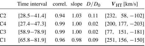
respec-Table 4. Results from the HT analysis. For each satellite one shows
the interval of analysis (in seconds from 07:36:00 UT), the correla-tion coefficient and the regression line slope between the electric field in the starting reference frameEi and the convection electric
fieldEHT= −VHT×B, the ratioD/D0expressing the fraction of
Ei remained un-transformed in the HT frame, and the three
com-ponents of the HT velocity,VHT, in GSE.
Time interval correl. slope D/D0 VHT[km/s]
C2 [28.5−41.4] 0.94 1.03 0.11 [232, 58,−102] C4 [27.4−47.3] 0.99 1.00 0.02 [200,177,−203] C3 [58.9−78.9] 0.99 1.00 0.02 [77, 151,−181] C1 [65.8−81.9] 0.96 0.98 0.09 [251,156,−150]
planar solutions imply, in case of C3 and C1, a systematic difference between the two sets of normals. The effect can be also noticed in the third and fourth panels of Figs. 8, 9 and 10. Actually, the analysis presented in Appendix B makes clear that this difference in orientation is due to the different time-intervals on which the two normals are based. In fact, in case of C3 and C1, for all centred intervals starting from [Tci−τi, Tci+τi]up to the largest one used in the analysis, the planar, interval-specific MVAB normals lie in the range of angular variation for the 2-D, instantaneous normals. This is exactly the result one expects when the planar MVAB tech-nique is applied to an ideal 2-D discontinuity (see Dunlop and Woodward, 1998).
5.3 Magnetopause normal velocity
Table 3 presents a comparison between the 2-D, non-planar method and the various planar techniques in terms of MP normal velocity prediction. In the planar case, we show the results obtained by combining the MVAB and HT analyses, those provided by the MFR analysis, by the two variants of the timing analysis, i.e. CTA and CVA, and by assuming a locally planar MP at each pair of consecutive satellites.
For the 24 June 2003 event, reasonably good HT frames at all four Cluster satellites were identified. Table 4 presents the results obtained from this analysis. For a meaningful com-parison with the 2-D method, the intervals of analysis (shown on column 2) were chosen as close as possible to the central crossing intervals[Tci−τi, Tci+τi]. In case of C1, C3 and C4 the plasma measurements together with the approxima-tion E= −v×B for the electric field were used, whereas for C2, where no ion plasma data are available, electric field measurements provided by the EFW instrument were em-ployed.
As Table 3 shows, by following the standard planar pro-cedure, i.e. projecting the HT velocities, VHT, on the nor-mals provided by the planar, nested MVAB analysis, one
[image:13.595.311.544.155.230.2]obtains values for the MP normal velocity significantly dif-ferent from theC2 OpTA Asolution. In fact, for C4 and C3, i.e. the satellites where the HT frame identification was most successful (see Table 4), these values are negative, which, considering that one deals with an in-bound transition, repre-sents an inconsistency. A possible explanation could be that in the HT analysis one tries to explain the observed electric field as being produced by a time-stationary structure mov-ing with constant velocity, both in direction and magnitude, relative to the point of observation, a situation one can hardly encounter in case of a 2-D MP8. The relatively small number of data points on which the HT analysis is based, i.e. five for both C4 and C3, could be another explanation.
The MFR method provides individual MP normal veloci-ties, VMFR, significantly higher than in the 2-D MP method. We have no particular explanation for this result; a more de-tailed investigation, like using synthetic data to study how the planar MFR method performs on a 2-D discontinuity, as done by Dunlop and Woodward (1998) for the MVAB technique, could prove to be useful.
The planar CTA and CVA timing techniques provide MP global normal velocities that are∼60 %, and, respectively ∼75% higher than in the 2-D MP method (see Tables 3 and 5 from Sect. 6).
The technique that evaluates the normal MP velocity by assuming a locally planar MP at each pair of consecutive satellites, provides results closer to theC2 OpTA Asolution for the first pair of satellites (C2 and C4), i.e. 55.3 compared to 54.2 km/s, respectively. For the next interval, between the C4 and C3 crossing times, the two methods provide signifi-cantly different results, i.e. 11.4 and 46.2 km/s, respectively. That can be explained by the large separation distance be-tween these satellites, when the effects of the MP curvature cannot be neglected. For the last pair of satellites (C3 and C1) the results are also significantly different, i.e. 22.9 and 40.7 km/s, respectively, in spite of their close separation. The reason for that resides in the difference between the indi-vidual MVAB normals, on which the calculation of Vpairis based, and the average geometrical normals based on the 2-D solution, i.e.n2Dave(see the last paragraph of Sect. 5.2).
6 Global parameters of the 2-D solutions
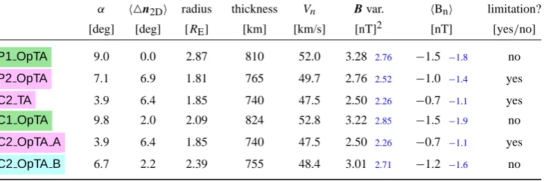
Table 5 presents the global values that characterize all six valid solutions obtained by applying different implementa-tions of the 2-D, non-planar method to the analyzed event. Two other solutions, namelyP2 TAandC1 TA, had to be 8One arrives at a similar conclusion when a version of HT
analy-sis that accounts for a possible accelerated motion of the HT frame (see Sonnerup et al., 1987) is used. For example, in case of C3, for the interval indicated in Table 4 (5 points) the instantaneous HT velocity projected on the nested MVAB normal is−13.9,−11.8, −9.8,−7.7,−5.6 km/s, giving an average MP normal velocity of −9.8 km/s.
abandoned because, although mathematically correct, they do not offer a physical description of the MP parameters and dynamics (see Blagau, 2007).
A close look at the corresponding MP macroscopic param-eters (thickness, normal velocity, radius of curvature, mag-netic variance) and at the general MP dynamics, yields simi-larities between these solutions. We therefore classified them in three groups, each indicated by a different color in Ta-ble 5. For the solutions belonging to the first group, i.e. for
P2 OpTA,C2 TA, andC2 OpTA A(pink background), the lowest values of the global normal magnetic field variance were obtained but one also needs to limit their range of va-lidity in order to avoid an artificial return of the first pair of satellites to the MP interior. The second group, consisting of the solutionsP1 OpTAandC1 OpTA(green background), imply a unidirectional displacement of the MP. The remain-ing solution, i.e.C2 OpTA B(blue background), implying two degrees of freedom for the MP movement, is not related with any other. Note that in Sect. 4 we presented one solution from each group.
On the first column of Table 5 we present the angleα, be-tween two normals already introduced in Sect. 4 and shown on Figs. 8, 9, and 10, namely the average normal provided by the nested, planar MVAB technique,hniMVAB, and a median MP normal provided by the 2-D solution, pointing to the ex-terior (in the geometrical sense),hniext. The parameter in the second column expresses the variation in the orientation of the 2-D instantaneous normals during the crossing intervals, being the average of 1n2D (see the description of Table 3 from Sect. 5).
The third and fourth columns present the values obtained for the MP radius of curvature and thickness, respectively. Since for a parabolic layer neither its radius of curvature nor its thickness are constant, the “global” values are shown, computed as geometrical mean (for the radius of curvature) or as arithmetical mean (for the thickness) of the correspond-ing individual quantities determined at each satellite9. Based on HIA C3 measurements, the average thermal proton gyro-radius for the MP interval is 133 km, and the average proton inertial length is 270 km.
The next column presents the MP global normal velocity, obtained as arithmetical mean of the individual average nor-mal velocity, vave2D. Then the global normal magnetic field variance and global value ofhBnicorresponding to the cen-tral intervals are shown. As in Table 3, the blue numbers des-ignate values based only on data from C1, C3 and C4, con-sidering that the C2 contribution to these global quantities is 9Actually, for a parabolic layer the individual values of these