www.biogeosciences.net/12/4621/2015/ doi:10.5194/bg-12-4621-2015
© Author(s) 2015. CC Attribution 3.0 License.
Deriving seasonal dynamics in ecosystem properties of semi-arid
savanna grasslands from in situ-based hyperspectral reflectance
T. Tagesson1, R. Fensholt1, S. Huber2, S. Horion1, I. Guiro3, A. Ehammer1, and J. Ardö4 1Department of Geosciences and Natural Resource Management, University of Copenhagen, Øster Voldgade 10, 1350 Copenhagen, Denmark
2DHI GRAS A/S, Agern Allé 5, 2970 Hørsholm, Denmark
3Laboratoire d’Enseignement et de Recherche en Géomatique, Ecole Supérieure Polytechnique, Université Cheikh Anta Diop de Dakar, BP 25275 Dakar-Fann, Senegal
4Department of Physical Geography and Ecosystem Science, Lund University, Sölvegatan 12, 223 62 Lund, Sweden
Correspondence to: T. Tagesson ([email protected])
Received: 11 December 2014 – Published in Biogeosciences Discuss.: 20 February 2015 Revised: 10 July 2015 – Accepted: 13 July 2015 – Published: 5 August 2015
Abstract. This paper investigates how hyperspectral re-flectance (between 350 and 1800 nm) can be used to infer ecosystem properties for a semi-arid savanna grassland in West Africa using a unique in situ-based multi-angular data set of hemispherical conical reflectance factor (HCRF) mea-surements. Relationships between seasonal dynamics in hy-perspectral HCRF and ecosystem properties (biomass, gross primary productivity (GPP), light use efficiency (LUE), and fraction of photosynthetically active radiation absorbed by vegetation (FAPAR)) were analysed. HCRF data (ρ) were used to study the relationship between normalised differ-ence spectral indices (NDSIs) and the measured ecosystem properties. Finally, the effects of variable sun sensor view-ing geometry on different NDSI wavelength combinations were analysed. The wavelengths with the strongest corre-lation to seasonal dynamics in ecosystem properties were shortwave infrared (biomass), the peak absorption band for chlorophylla andb (at 682 nm) (GPP), the oxygen A band at 761 nm used for estimating chlorophyll fluorescence (GPP and LUE), and blue wavelengths (ρ412) (FAPAR). The NDSI with the strongest correlation to (i) biomass combined red-edge HCRF (ρ705) with green HCRF (ρ587), (ii) GPP com-bined wavelengths at the peak of green reflection (ρ518, ρ556), (iii) LUE combined red (ρ688) with blue HCRF (ρ436), and (iv) FAPAR combined blue (ρ399) and near-infrared (ρ1295) wavelengths. NDSIs combining near infrared and shortwave infrared were strongly affected by solar zenith
an-gles and sensor viewing geometry, as were many combina-tions of visible wavelengths. This study provides analyses based upon novel multi-angular hyperspectral data for val-idation of Earth-observation-based properties of semi-arid ecosystems, as well as insights for designing spectral char-acteristics of future sensors for ecosystem monitoring.
1 Introduction
Gower et al., 1999; Sjöström et al., 2009; Sims and Gamon, 2003). In situ observations of spectral reflectance are also important for parameterisation and validation of canopy re-flectance models, as well as space- and airborne products (Coburn and Peddle, 2006).
Very few sites across the world exist with an instrumen-tal setup designed for multi-angular continuous hyperspec-tral measurements. Leuning et al. (2006) present a system mounted in a 70 m tower above an evergreen eucalyptus for-est in New South Wales, Australia, which measures spectral hemispherical conical reflectance factors (HCRFs)1 hourly throughout the year between 300 and 1150 nm at four az-imuth angles. Hilker et al. (2007, 2010) describe an au-tomated multi-angular spectro-radiometer for estimation of canopy HCRF (AMSPEC) mounted on a tower above a coniferous forest in Canada. Spectral HCRF is sampled be-tween 350 and 1200 nm year-round under different viewing and sun angle conditions, achieved by collection of data in a near 360◦view around the tower with adjustable viewing zenith angles. Even though in situ measurements of multi-angular hyperspectral HCRF are fundamental for the EO re-search community, such data sets are still rare and, at the present state, they do not cover different biomes at the global scale (Huber et al., 2014).
There are many methods for analysing relationships be-tween hyperspectral reflectance and ecosystem properties, such as multivariate methods, derivative techniques, and ra-diative transfer modelling (Bowyer and Danson, 2004; Cec-cato et al., 2002; Danson et al., 1992; Roberto et al., 2012). Still, due to its simplicity, the combination of reflectance into vegetation indices is the major method for upscaling using EO data. By far, the most commonly applied vege-tation indices are those based on band ratios, e.g. the nor-malised difference vegetation index (NDVI), which is calcu-lated by dividing the difference in the near-infrared (NIR) and red wavelength bands by the sum of the NIR and red bands (Tucker, 1979; Rouse et al., 1974). The NIR radiance is strongly scattered by the air–water interfaces between the cells, whereas red radiance is absorbed by chlorophyll and its accessory pigments (Gates et al., 1965). The normalisa-tion with the sum in the denominator is a means to reduce the effects of solar zenith angle, sensor viewing geometry, and atmospheric errors as well as enhancing the signal of the observed target (e.g. Qi et al., 1994; Inoue et al., 2008).
Wavelength specific spectral reflectance is known to be re-lated to leaf characteristics such as chlorophyll concentra-1Different reflectance terminologies have been used to inform
on spectral measurements in the field by the remote sensing com-munity leading to suggestions to the proper use of the terminol-ogy (Martonchik et al., 2000). All field spectro-radiometers mea-sure HCRF (hemispherical conical reflectance) if the field of view (FOV) of the sensor is larger than 3◦(Milton et al., 2009). HCRF is therefore used throughout this paper to support the correct in-ference and usage of reflectance products (Schaepman-Strub et al., 2006; Milton et al., 2009).
tion, dry matter content, internal structure parameters, and equivalent water thickness (Ceccato et al., 2002). Hyper-spectral reflectance data can be combined into a matrix of normalised difference spectral indices (NDSIs), following the NDVI rationing approach. Correlating the NDSI with ecosystem properties provides a way to gain an improved empirically based understanding of the relationship between information in the reflectance spectrum with ground surface properties (e.g. Inoue et al., 2008). Several studies have anal-ysed relationships between hyperspectral HCRF, NDSI, and ecosystem properties (e.g. Thenkabail et al., 2000; Cho et al., 2007; Psomas et al., 2011; Inoue et al., 2008; Gamon et al., 1992; Feret et al., 2008; Thenkabail et al., 2012). Still, it is extremely important to examine these relationships for dif-ferent ecosystems across the Earth and investigate their ap-plicability for different environmental conditions and under different effects of biotic and abiotic stresses.
A strong correlation between an NDSI and an ecosys-tem property does not necessarily indicate that the NDSI is a good indicator of vegetation conditions to be applied to EO systems. Visible, NIR, and shortwave infrared (SWIR) have different sensitivity to variations in solar zenith angles, stand structure, health status of the vegetation, vegetation and soil water content, direct/diffuse radiation ratio, and sensor viewing geometry. The influence of sun–sensor geometry on the reflected signal has been studied using radiative trans-fer models and airborne (e.g. AirMISR) as well as satellite-based data from instruments such as CHRIS-PROBA, MISR, or POLDER (Huber et al., 2010; Maignan et al., 2004; Javier García-Haro et al., 2006; Jacquemoud et al., 2009; Verhoef and Bach, 2007; Laurent et al., 2011). However, effects of variable sun angles and sensor viewing geometries are not well documented in situ for different plant functional types of natural ecosystems except for some individual controlled experiments (Hilker et al., 2008; Sandmeier et al., 1998; Schopfer et al., 2008). Improved knowledge regarding the in-fluence from sun–sensor variability on different NDSI com-binations is thereby essential for validating the applicability of an NDSI for EO upscaling purposes.
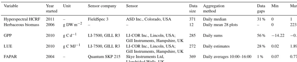
Table 1. Information about the instrumental setup for the measured environmental variables. HCRF is hemispherical conical reflectance
factor, GPP is gross primary productivity, LUE is light use efficiency, and FAPAR is fraction of photosynthetically active radiation absorbed by the vegetation. Min and Max are minimum and maximum values measured, respectively, DW is dry weight, C is carbon, and MJ is megajoules. The year started is the first year with measurements. Time is in UTC. For more information about the instrumental setup, see Tagesson et al. (2015b).
Variable Year Unit Sensor company Sensor Data Aggregation Data Min Max
started size method gaps
Hyperspectral HCRF 2011 – FieldSpec 3 ASD Inc., Colorado, USA 371 Daily median 31 % 0 1 Herbaceous biomass 2006 g DW m−2 – – 12 Daily mean 28 plots – 0 223
GPP 2010 g C d−1 LI-7500, GILL R3 LI-COR Inc., Lincoln, USA; 285 Daily sums 56 % −14.22 −0.22
Gill Instruments, Hampshire, UK
LUE 2010 g C MJ−1 LI-7500, GILL R3 LI-COR Inc., Lincoln, USA; 272 Daily estimates 28 % 0.02 1.89
Gill Instruments, Hampshire, UK
FAPAR 2004 – Quantum SKP 215 Skye Instruments Ltd, 369 Daily averages 10:00–16:00 1 % 0.07 0.77 Llandridod Wells, UK
with different wavelength combinations (350 to 1800 nm) and the measured ecosystem properties, and (iii) to analyse and quantify effects of variable sun angles and sensor view-ing geometries on different NDSI combinations.
2 Materials and method 2.1 Site description
All measurements used for the present study were conducted at the Dahra field site in the Sahelian ecoclimatic zone north-east of the town Dahra in the semi-arid central part of Senegal (15◦2401000N, 15◦2505600W) during 2011 and 2012 (Fig. 1). Rainfall is sparse in the region, with a mean annual sum of 416 mm (1951–2003). More than 95 % of the rain falls between July and October, with August being the wettest month. The mean annual air temperature is 29◦C (1951– 2003); May is the warmest month and January the cold-est, with mean monthly temperatures of 32 and 25◦C, re-spectively. The Dahra site has a short growing season (∼3 months) following the rainy season, with leaf area index generally ranging between 0 and 2 (Fensholt et al., 2004). South-western winds dominate during the rainy season and north-eastern winds during the dry season. The area is dom-inated by annual grasses (e.g. Schoenefeldia gracilis,
Dig-itaria gayana, Dactyloctenium aegypticum, Aristida muta-bilis, and Cenchrus biflorus) (Mbow et al., 2013), and trees
and shrubs (e.g. Acacia senegal and Balanites aegyptiaca) are relatively sparse (∼3 % of the land cover) (Rasmussen et al., 2011). The average tree height was 5.2 m and the peak height of the herbaceous layer was 0.7 m (Tagesson et al., 2015b). A thorough description of the Dahra field site is given in Tagesson et al. (2015b).
2.2 Meteorological and vegetation variables
A range of meteorological variables have been measured from a tower at the Dahra field site for more than 10 years: air temperature (◦C) and relative humidity (%) were
mea-sured at 2 m height; soil temperature (◦C) and soil moisture (volumetric water content (m3m−3×100) (%)) were col-lected at 0.05 m depths; rainfall (mm) was measured at 2 m height; incoming (inc) and reflected (ref) PAR (µmol m−2s−1) was measured at 10.5 m height; and PAR transmitted through the vegetation (PARtransmit) was measured at six plots at ∼0.01 m height (Table 1) (Tagesson et al., 2015b). The PARtransmit was measured within a distance of 7 m from the tower. PAR absorbed by the vegetation (APAR) was esti-mated by
APAR=PARinc−PARref−(1−αsoil)×PARtransmit, (1) whereαsoil is the PAR albedo of the soil, which was mea-sured as 0.20 (Tagesson et al., 2015b). FAPAR was estimated by dividing APAR by PARinc (Tagesson et al., 2015b). All sensors were connected to a CR-1000 logger in combination with a multiplexer (Campbell Scientific Inc., North Logan, USA). Data were sampled every 30 s and stored as 15 min averages (sum for rainfall).
Figure 1. Map and photos of the Dahra field site and measured areas. The map shows the location of Dahra within the Sahel (orange
area). (a) Photo of the footprint of the eddy covariance (EC) tower; (b) photo of the EC tower; (c) photo of the meteorological tower with the spectroradiometers; (d) photo of the instantaneous field of view (IFOV) of the spectroradiometers during the rainy season; (e) photo of the IFOV of the spectroradiometer during the beginning of the dry season; and (f) Quickbird image from the Dahra field site from 11 September 2011 showing the location of the meteorological tower, the EC tower, the biomass sampling plots, and the footprint of the EC measurements. The EC footprint area is the median 70 % cumulative flux distance from the eddy covariance tower. The photos of the EC tower and its footprint are taken during the rainy season, whereas the photo of the meteorological tower shows the late dry season.
2.3 Estimates of gross primary productivity and light use efficiency
Net ecosystem exchange of CO2(NEE) (µmol CO2m−2s−1) was measured with an eddy covariance system, consisting of an open-path infrared gas analyser (LI-7500, LI-COR Inc., Lincoln, USA) and a three-axis sonic anemometer (Gill in-struments, Hampshire, UK) from 18 July 2011 until 31 De-cember 2012 (Table 1). The sensors were mounted 9 m above the ground on a tower (placed 50 m south of the tower in-cluding the meteorological and spectroradiometric sensors)
ef-fects (Moncrieff et al., 2004). The data were filtered for steady state and fully developed turbulent conditions, follow-ing Foken et al. (2004), and accordfollow-ing to statistical tests as recommended by Vickers and Mahrt (1997). Flux measure-ments from periods of heavy rainfall were also removed. For a thorough description of the post processing of the raw eddy covariance data, see Tagesson et al. (2015a).
A possible source of error in a comparison between EC-based variables and spectral HCRF is the difference in foot-print/instantaneous field of view (IFOV) between the sensors. The IFOV of the spectroradiometer setup contains only soil and herbaceous vegetation. The footprint of the EC tower was estimated using a model based on measurement height, surface roughness, and atmospheric stability (Hsieh et al., 2000). The median point of maximum contribution is at 69 m, and the median 70 % cumulative flux distance is at 388 m from the tower. The footprint of the EC tower contains semi-arid savanna grassland with∼3 % tree coverage, and the EC data are thereby affected by both woody and herba-ceous vegetation (Fig. 1a and f). But given the low tree cov-erage, and the dominant influence of herbaceous vegetation on the seasonal dynamics in CO2fluxes, we still consider it reasonable to compare EC fluxes with seasonal dynamics in spectral HCRF of the herbaceous vegetation.
The daytime NEE was partitioned into GPP and ecosys-tem respiration using the Mitscherlich light-response func-tion against PARinc(Falge et al., 2001). A 7-day moving win-dow with 1-day time steps was used when fitting the func-tions. By subtracting dark respiration (Rd) from the light-response function, it was forced through 0, and GPP was es-timated:
GPP= −(Fcsat+Rd)×
1−e
−α×PARinc
Fcsat+Rd
, (2)
where Fcsat is the CO2 uptake at light saturation (µmol CO2m−2s−1) andα is the quantum efficiency or the ini-tial slope of the light-response curve (µmol CO2 (µmol photons)−1) (Falge et al., 2001). Vapour pressure deficit (VPD) limits GPP and to account for this effect, the Fcsat parameter was set as an exponentially decreasing function:
Fcsat=
Fcsat×e−k(VPD−VPD0) VPD>VPD0
Fcsat VPD<VPD0
(3) where VPD0 is 10 hPa following the method by Lasslop et al. (2010).
Gaps in GPP less than or equal to 3 days were filled us-ing three different methods: (i) gaps shorter than 2 h were filled using linear interpolation, (ii) daytime gaps were filled by using the light-response function for the 7-day moving windows, and (iii) remaining gaps were filled by using mean diurnal variation 7-day moving windows (Falge et al., 2001). A linear regression model was fitted between daytime GPP and APAR for each 7-day moving window to estimate LUE, where LUE is the slope of the line.
2.4 Hyperspectral HCRF measurements and NDSI estimates
Ground surface HCRF spectra were measured every 15 min between sunrise and sunset from 15 July 2011 until 31 De-cember 2012 using two FieldSpec 3 spectrometers with fibre optic cables (Table 1) (ASD Inc., Colorado, USA). The spec-troradiometers cover the spectral range from 350 to 1800 nm and have a FOV of 25◦. The spectral resolution is 3 nm at 350–1000 nm and 10 nm at 1000–1800 nm and the sam-pling interval is 1.4 nm at 350–1000 nm and 2 nm at 1000– 1800 nm. From these data, 1 nm spectra were calculated by using cubic spline interpolation functions. One sensor head was mounted on a rotating head 10.5 m above the surface (at the same tower including instruments to measure meteoro-logical variables), providing measurements of the herbaceous vegetation from seven different viewing angles in a transect underneath the tower (nadir, 15, 30, and 45◦off-nadir angles towards east and west). No trees or effects of shading of trees are present in the IFOV of the data used in this study (Fig. 1). A reflective cosine receptor is used to measure full-sky irra-diance by having the second sensor head mounted on a 2 m high stand pointing to a Spectralon panel (Labsphere Inc., New Hampshire, USA) under a glass dome.
NDSI using all possible combinations of two separate wavelengths were calculated as
NDSI= ρi −ρj
ρi+ρj
, (4)
whereρiandρj are the daily median HCRF in two separate
single wavelengths (iandj) between 350 and 1800 nm. In
or-der to minimise the influence of errors we used daily median hyperspectral HCRF in the analysis (since the median pro-vides the most common model output and is thereby more robust against outliers than average values).
2.5 Effects of varying sun and sensor viewing geometry on NDSI
The effects of variable solar zenith angles on different NDSI combinations were studied with nadir HCRF measurements. In order to capture the seasonal dynamics, data were taken over 15 days during four periods: (1) the dry season in 2012 (day of year (DOY) 71–85), (2) the fast growth period in 2011 (start of the rainy season) (DOY 200–214), (3) the peak of the growing season in 2011 (DOY 237–251), and (4) the senescent period in 2011 (the end of the rainy season) (DOY 278–293). Only days with full data coverage were used in order not to include bias in the results from days with incom-plete data sets. The median HCRF of the 15 days was cal-culated for each wavelength for every 15 min between 08:00 and 18:00 (UTC). These HCRF values were combined into NDSI with different wavelength combinations. Finally, daily mean and standard deviation for all wavelength combinations were calculated. Diurnal variability in the NDSI was assessed with the coefficient of variation (COV), which is the ratio be-tween the standard deviation and the mean. The COV gives an indication of effects related to variable solar zenith angles. To capture directional effects in the NDSI related to the variable view zenith angles (15, 30, and 45◦off-nadir angles towards east and west) the NDSI was calculated using me-dian HCRF values from the four above-mentioned periods for the different viewing angles. Only data measured between 12:00 and 14:00 (UTC) were used so as to avoid effects of variable solar zenith angles. The anisotropy factor (ANIF) is defined as the fraction of a reflected property at a specific view direction relative to the nadir, and it was calculated by ANIF(λ, θ )=NDSI(λ, θ )
NDSI0(λ)
, (5)
where NDSI(λ, θ) is NDSI for the different wavelengths (λ) and the different viewing angles (θ), and NDSI0(λ) is the nadir-measured NDSI (Sandmeier et al., 1998).
2.6 Relationship between hyperspectral HCRF, NDSI, and ecosystem properties
We examined the relationship between predictor variables (daily median hyperspectral HCRF, and NDSI from nadir
observations) and response variables (biomass, GPP, LUE, and FAPAR). A comparison between fitted linear and ex-ponential regression models indicated no improvement by fitting exponential regression models; we hence choose to use linear regression analysis (Supplement). Possible er-rors (random sampling erer-rors, aerosols, dust or water on the sensor heads, electrical senor noise, filtering and gap-filling errors, errors in correction factors, sensor drift, and instrumentation errors) can be present in predictor and re-sponse variables. We thereby used a reduced major axis lin-ear regression to account for errors in both the predictor and response variables when fitting the regression lines. In order to estimate the robustness of the empirical relation-ships, we used a bootstrap simulation methodology, where the data sets were copied 200 times (Richter et al., 2012). The runs generated 200 sets of slopes, intercepts, and co-efficients of determination (R2), from which the median and standard deviation were estimated. The generated sta-tistical models were validated against the left-out subsam-ples within the bootstrap simulation method by calculating the root-mean-square error (RMSE) and the relative RMSE (RRMSE=100×RMSE×mean(observed)−1); median and standard deviation were estimated. Within the regression analysis, all variables used were repeated observations of the same measurement plot. The dependent and independent variables are hence temporally autocorrelated and cannot be regarded as statistically independent. We thereby choose not to present any statistical significance. The analyses, however, still indicate how closely coupled the explanatory variables are with the ecosystem properties.
A filter was created for the analysis between NDSI and ecosystem properties; all NDSI combinations with a COV higher than 0.066 in any of the four periods (dry season, fast growth period, peak of the growing season, and senes-cent period) and all NDSI combinations with ANIF values higher than 1.2 and lower than 0.8 in any of the four periods were filtered. The ANIF thresholds of 1.2 and 0.8 and the COV threshold of 0.066 were used since values then vary less than 20 % due to effects of variable sun–sensor geometry. NDSI including the water absorption band (1300–1500 nm) was also removed as it is strongly sensitive to atmospheric water content and is less suitable for spatial extrapolation of ecosystem properties using air/spaceborne sensors (Asner, 1998). Finally, NDSI combinations including wavelengths between 350 and 390 nm were removed owing to low signal-to-noise ratio in the ASD sensors (Thenkabail et al., 2004).
3 Results
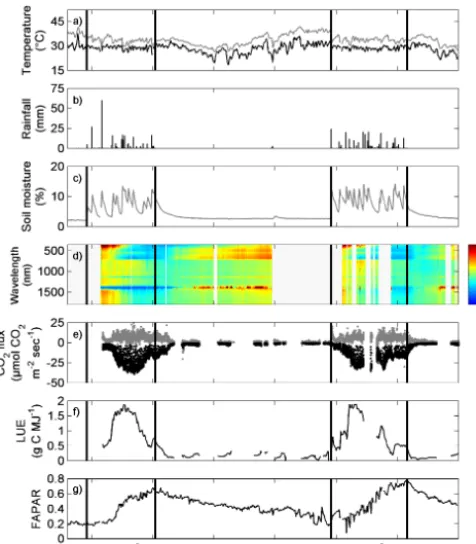
val-Figure 2. Time series of the measured variables: (a) daily averaged
air temperature (black line), as well as soil temperature at 0.05 m depth (grey line); (b) daily sums of rainfall; (c) daily average of soil moisture at 0.05 m depth; (d) hyperspectral hemispherical con-ical reflectance factor (HCRF) normalised by calculating the ratio between daily median HCRF for each wavelength (350–1800 nm) and the average HCRF for the entire measurement period; (e) gross primary productivity (GPP) (black dots) and ecosystem respiration (grey dots); (f) the light use efficiency (LUE); and (g) the fraction of photosynthetically active radiation absorbed by the vegetation (FAPAR). The black vertical lines are the start and end of the rainy seasons (first and final day of rainfall). The gaps are caused by tech-nical issues due to loss of power supply, broken sensors, or filtering of data due to bad weather conditions.
ues at the end of the dry season (Fig. 2a). Yearly rainfall was 486 and 606 mm for 2011 and 2012, respectively. Soil mois-ture ranged between 1.9 and 14.1 %, and it clearly followed the rainfall patterns (Fig. 2b and c). The CO2fluxes were low during the dry period and high during the rainy season (July– October) (Fig. 2e). The LUE followed GPP closely (Fig. 2f). FAPAR was low at the start of the rainy season, followed by a maximum towards the end of the rainy season, and then slowly decreased over the dry season (Fig. 2g).
[image:7.612.305.550.65.256.2]The range in HCRF is large across the spectral space, and would hide the seasonal dynamics in hyperspectral HCRF if directly shown. Therefore, to clearly illustrate these seasonal dynamics, the ratio between daily median nadir HCRF and the average HCRF for the entire measurement period was calculated for each wavelength (350–1800 nm). This gives a fraction of how the HCRF for each wavelength varies over
Figure 3. The coefficient of variation (COV), i.e. the ratio between
daily standard deviation and the daily mean (measurements taken between 08:00 and 18:00 (UTC)), for different normalised differ-ence spectral index (NDSI) wavelength (i, j) combinations for 12 days at the peak of the growing season 2011 (day of year 237–251;
n=576). The COV indicates how strongly the NDSI are affected by variable sun angles. The upper right half of the chart shows the unfilteredR2values, whereas the lower left half shows filteredR2, based on the filtering criteria described in Sect. 2.6.
the measurement period in relation to the average of the en-tire period (Fig. 2d). In the visible (VIS) part of the spec-trum (350–700 nm) there was a stronger absorption during the second half of the rainy season and at the beginning of the dry season than during the main part of the dry season and the start of the rainy season. There was stronger NIR ab-sorption (700–1300 nm) at the end of the rainy season and the beginning of the dry season, whereas the absorption de-creased along with the dry season. Strong seasonal variation was observed in the water absorption region around 1400 nm following the succession of rainy and dry seasons. HCRF in the SWIR (1400–1800 nm) generally followed the seasonal dynamics of the visible part of the spectrum.
3.2 Effects of sensor viewing geometry and variable sun angles on NDSI
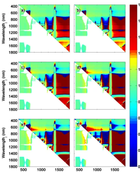
[image:7.612.51.289.67.339.2]Figure 4. The anisotropy factor (ANIF) for different normalised
difference spectral index (NDSI) wavelength (i, j) combinations for
15 days at the peak of the growing season 2011 (day of year 237– 251) for the different sensor viewing angles: (a) 15◦E, (b) 15◦W,
(c) 30◦E, (d) 30◦W, (e) 45◦E, and (f) 45◦W. In order not to include effects of solar zenith angles in the analysis, only data measured between 12:00 and 14:00 (UTC) were used in the ANIF calculations (n=48). The upper right half of each chart shows the unfilteredR2
values, whereas the lower left half shows filteredR2, based on the filtering criteria described in Sect. 2.6.
combinations, as well as for VIS wavelengths between 550 and 700 nm (Fig. 4). Remaining VIS wavelengths were less affected. It was also clear that ground surface anisotropy in-creased strongly as a function of increasing viewing angle (Fig. 4). Moreover, some band combinations showed already angular sensitivity at view zenith angles of 15◦, while other band combinations only manifest anisotropic behaviour with higher view angles. Some band combinations, however, do not show any increased anisotropy at all (areas coloured in green in all six plots).
3.3 Relationship between hyperspectral HCRF, NDSI, and ecosystem properties
3.3.1 Biomass
[image:8.612.329.525.69.484.2]HCRF values for all wavelengths except the water absorp-tion band at 1100 nm were strongly correlated with biomass
Figure 5. Median correlation coefficient (±1 SD) between seasonal dynamics in hyperspectral hemispherical conical reflectance factors (HCRF) 2011–2012 and (a) dry weight biomass (n=12; g m−2),
(b) gross primary productivity (GPP) (n=285; g C day−1), (c) light use efficiency (LUE) (n=272; g C MJ−1), and (d) fraction of pho-tosynthetically active radiation absorbed by the vegetation (FA-PAR) (n=369). The water absorption band (1300–1500 nm) was removed as it is strongly sensitive to atmospheric water content, and wavelengths between 350 and 390 nm were removed owing to low signal-to-noise ratio in the ASD sensors.
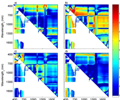
pos-Figure 6. Coefficient of determination (R2) between normalised difference spectral index (NDSI) and (a) dry weight biomass (n=12; g m−2), (b) gross primary productivity (GPP) (n=285; g C day−1), (c) light use efficiency (LUE) (n=272; g C MJ −1), and (d) fraction of photosynthetically active radiation absorbed by the vegetation (FAPAR) (n=369). The upper right half of each chart shows the unfilteredR2values, whereas the lower left half shows filteredR2, based on the filtering criteria described in Sect. 2.6.
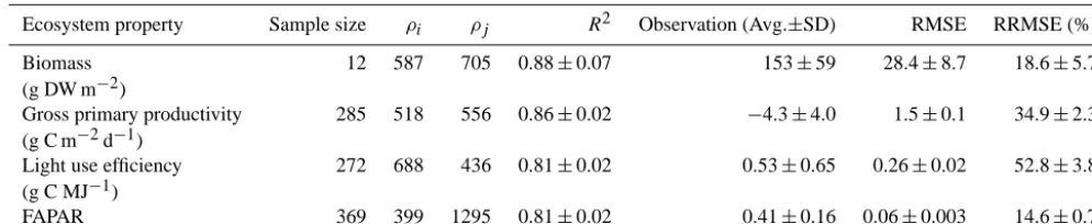
itive correlation is seen at 1120–1150 nm. NDSI combina-tions with HCRF in the red edge (ρ680–ρ750) and HCRF in the VIS region explained seasonal dynamics in biomass well (Fig. 6a). The strongest relationship (R2=0.88±0.07; RRMSE=18.6±5.7 %) between NDSI and biomass was found for NDSI combining 705 and 587 nm (NDSI[705, 587]) (Table 2, Fig. 7a).
3.3.2 Gross primary productivity
[image:9.612.47.288.66.268.2]The relationship between GPP and nadir-measured hyper-spectral HCRF is inverted as compared to other correlation coefficient lines (Fig. 5b), since GPP is defined as a with-drawal of CO2from the atmosphere with higher negative val-ues for a larger CO2uptake. The seasonal dynamics in GPP was strongly positively correlated with HCRF in the blue, red, SWIR wavelengths, and the water absorption band at 1100 nm, whereas it was strongly negatively correlated with the NIR HCRF. The study revealed the strongest positive and negative correlations for HCRF at 682 nm (r=0.70±0.02) and 761 nm (r= −0.74±0.02), respectively. NDSI com-binations that explained most of the GPP variability were different combinations of the VIS and NIR or red and SWIR wavelengths (Fig. 6b). However, the strongest re-lationship was seen at NDSI[518, 556] (R2=0.86±0.02; RRMSE=34.9±2.3 %) (Table 2; Fig. 7b).
Figure 7. The least-squares linear regressions with the strongest
relationships between the normalised difference spectral index (NDSI) and (a) dry weight biomass, (b) gross primary productivity (GPP), (c) light use efficiency (LUE), and (d) fraction of photosyn-thetically active radiation absorbed by the vegetation (FAPAR). In the equations, the slope and intercepts (±1 SD) is given.
3.3.3 Light use efficiency
LUE was negatively correlated with HCRF in the blue and red spectral ranges and in the water absorption band at 1100 nm, and it was positively correlated in the NIR wave-lengths (Fig. 5c). HCRF at 761 nm yielded the strongest pos-itive correlation (r=0.87±0.01). When combining the dif-ferent wavelengths to NDSI, the VIS wavelengths explained variation in LUE well, with the strongest relationships in the red and blue parts of the spectrum (Fig. 6c). LUE corre-lated most strongly with NDSI[436, 688] (R2=0.81±0.02; RRMSE=52.8±3.8 %)) (Table 2; Fig. 7c).
3.3.4 Fraction of photosynthetically active radiation absorbed by the vegetation
[image:9.612.306.550.66.230.2]Table 2. Wavelengths of the hemispherical conical reflectance factors (HCRF) (ρi, j; nm) used in the normalised difference spectral indices
(NDSI) that generated the strongest correlations with ecosystem properties. DW is dry weight, FAPAR is the fraction of photosynthetically active radiation absorbed by the vegetation, Avg. is average, SD is standard deviation, RMSE is root-mean-square error, and RRMSE is relative RMSE.
Ecosystem property Sample size ρi ρj R2 Observation (Avg.±SD) RMSE RRMSE (%)
Biomass 12 587 705 0.88±0.07 153±59 28.4±8.7 18.6±5.7 (g DW m−2)
Gross primary productivity 285 518 556 0.86±0.02 −4.3±4.0 1.5±0.1 34.9±2.3 (g C m−2d−1)
Light use efficiency 272 688 436 0.81±0.02 0.53±0.65 0.26±0.02 52.8±3.8 (g C MJ−1)
FAPAR 369 399 1295 0.81±0.02 0.41±0.16 0.06±0.003 14.6±0.7
4 Discussion
4.1 Effects of sensor viewing geometry and variable sun angles on the NDSI
Effects of solar zenith angles and sensor viewing geometry were similar (Figs. 3 and 4), since they affect HCRF mea-surements in a similar way (Kimes, 1983). In dense and erec-tophile canopies, HCRF increases with sensor viewing and solar zenith angles, because a larger fraction of the upper vegetation canopy is viewed/illuminated, whereas the shad-owed lower part of the canopy contributes less to the mea-sured signal as shown previously by several studies (Huete et al., 1992, 2014; Jin et al., 2002; Kimes, 1983). However, the radiative transfer within a green canopy is complex, and differs across the spectral region (Huber et al., 2014). Less radiation is available for scattering of high-absorbance spec-tral ranges (such as the VIS wavelengths), and this tends to increase the contrast between shadowed and illuminated ar-eas for these wavelengths, wherar-eas in the NIR and SWIR ranges, more radiation is scattered and transmitted, which thereby decreases the difference between shadowed and illu-minated areas within the canopy (Kimes, 1983; Hapke et al., 1996). A recognised advantage of NDSI calculations is that errors/biases that are similar in both wavelengths included in the index are suppressed by the normalisation. However, for a given situation where errors/biases are different for the wavelengths used, such as effects generated by sun–sensor geometry, errors/biases will affect the value of the index. This was also the case at the Dahra field site: NDSI val-ues were strongly affected at wavelength combinations with large differences in effects of variable solar zenith angles (Fig. 6 in Huber et al., 2014) and variable view zenith an-gles (Fig. 4 in Tagesson et al., 2015b). This effect is espe-cially pronounced in the case of low index values (closer to 0), whereas larger index values (closer to 1 and−1) become less sensitive. The relative HCRF difference between NIR and SWIR is lower compared to indices including the VIS domain; NIR/SWIR-based indices thereby generate lower NDSI values with higher sensitivity to sun–sensor
geometry-generated differences between included wavelengths (Figs. 3 and 4). This can also be seen in the SIWSI–NDVI compari-son by Huber et al. (2014); SIWSI had large relative differ-ences depending on viewing angle (∼70 %), whereas NDVI had relatively small differences (∼5 %) (Fig. 10 in Huber et al., 2014). Fensholt et al. (2010a) showed the same to be true in a comparison between SIWSI and NDVI based on MODIS data: SIWSI was insensitive to day-to-day variations in canopy water status due to effects of solar zenith angles and sensor viewing geometry blurring the signal.
A strong diurnal dynamic does not necessarily mean a poor NDSI. For example, the photochemical reflectance in-dex (PRI) was created for assessing diurnal dynamics in the xanthophyll cycle activity (Gamon et al., 1992). Stomatal closure due to high temperatures could also influence diurnal dynamics of vegetation properties (Lasslop et al., 2010), and hence the diurnal dynamics of NDSI. However, diurnal varia-tion in reflectance caused by diurnal variability in vegetavaria-tion status is assumed minor in relation to the diurnal variability caused by changes in solar zenith angles. Additionally, in our study we are interested in relationships in seasonal dynamics between ecosystem properties and NDSI; diurnal variation can thereby interfere and introduce uncertainty into such re-lationships.
reflectance distribution function) modelling (Jacquemoud et al., 2009; Bicheron and Leroy, 2000). The multi-angular data set is also highly valuable for evaluation and validation of satellite-based products, where the separation of view an-gle and atmospheric effects can only be done using radiative transfer models (Holben and Fraser, 1984).
4.2 Seasonal dynamics in hyperspectral HCRF, NDSI, and ecosystem properties
4.2.1 Biomass
The strong correlation between biomass and most of the spectrum indicates the strong effects of phenology on the sea-sonal dynamics in the HCRF spectra (Fig. 5a). Variability in VIS (350–700 nm) HCRF for vegetated areas is strongly re-lated to changes in leaf pigments (Asner, 1998), and this can also be seen in Fig. 2d since absorption was much stronger during the rainy (growing) season than during the dry sea-son. Previous studies have generally shown positive relation-ships between NIR HCRF and biomass since a large frac-tion of NIR radiafrac-tion is reflected in green healthy vegeta-tion to avoid overheating (e.g. Hansen and Schjoerring, 2003; Asner, 1998). Here, a strong negative relationship between NIR HCRF and dry weight biomass is generally observed (Fig. 5a), indicating stronger NIR absorption with increased biomass. However, a strong positive NIR HCRF correlation with vegetation water content was seen (figure not shown). A possible explanation could be that the sampled biomass at the end of the rainy season contained some senescent vegetation, and a correlation against vegetation water content is hence closer to green healthy vegetation. This relationship is, how-ever, interesting and should be studied further to better un-derstand the respective importance of canopy water and leaf internal cellular structure for the NIR HCRF of herbaceous vegetation characterised by erectophile leaf angle distribu-tion in semi-arid regions. We found the strongest correladistribu-tion for biomass with a SWIR wavelength, thereby confirming the studies by Lee (2004) and Psomas et al. (2011) in that SWIR wavelengths are good predictors of LAI or biomass.
The NDVI is known to saturate at high biomass because the absorption of red light at ∼680 nm saturates at higher biomass loads, whereas the NIR HCRF continues to increase due to multiple scattering effects (Mutanga and Skidmore, 2004; Jin and Eklundh, 2014). Several studies have shown that NDSI computed with narrowband HCRF improve this relationship by choosing a wavelength region not as close to the maximum red absorption at∼680 nm, for example using shorter and longer wavelengths of the red edge (700–780nm) (Cho et al., 2007; Mutanga and Skidmore, 2004; Lee, 2004) and NIR and SWIR wavelengths (Psomas et al., 2011; Lee, 2004). The NDSI with the strongest correlation to biomass was computed using red-edge HCRF (ρ705) and green HCRF (ρ587). Vegetation stress and information about chlorophyll and nitrogen status of plants can be extracted from the
red-edge region (Gitelson et al., 1996). Wavelengths aroundρ550 are located right at the peak of green reflection and closely related to the total chlorophyll content, leaf nitrogen content, and chlorophyll/carotenoid ratio and have previously been shown to be closely related to biomass (Inoue et al., 2008; Thenkabail et al., 2012).
4.2.2 Gross primary productivity
The maximum absorption in the red wavelengths generally occurs at 682 nm as this is the peak absorption for chloro-phylla andb (Thenkabail et al., 2000), and this was also the wavelength that was most strongly correlated with GPP. HCRF at 682 nm was previously shown to be strongly re-lated to LAI, biomass, plant height, NPP, and crop type dis-crimination (Thenkabail et al., 2004, 2012). The NDSI with the strongest relationship to GPP was based on HCRF in the vicinity of the green peak. The PRI normalises HCRF at 531 and 570 nm and it was suggested for detection of di-urnal variation in the xanthophyll cycle activity (Gamon et al., 1992), and it is commonly used for estimating produc-tivity efficiency of the vegetation (e.g. Soudani et al., 2014). The present study thereby confirms the strong applicability of the wavelengths in the vicinity of the green peak for veg-etation productivity studies. Again, wavelengths around the green peak are related to the total chlorophyll content, leaf nitrogen content, chlorophyll / carotenoid ratio, and biomass (Inoue et al., 2008; Thenkabail et al., 2012).
4.2.3 Light use efficiency
Both LUE and GPP were most strongly correlated with HCRF at 761 nm, which is the oxygen A band within the NIR wavelengths. HCRF at 761 nm is commonly used for estimating solar-induced chlorophyll fluorescence due to ra-diation emitted by the chlorophyll, and it has been suggested as a direct measure of health status of the vegetation (Meroni et al., 2009). Earth observation data for estimating fluores-cence should have very high spectral resolution (<10 nm), but considering the rapid technical development within sen-sors for hyperspectral measurements, fluorescence possibly has strong practical potential for monitoring vegetation status (Meroni et al., 2009; Entcheva Campbell et al., 2008). Glob-ally mapped terrestrial chlorophyll fluorescence retrievals are already produced from the GOME-2 instrument at a spatial resolution of 0.5◦×0.5◦, but hopefully this will also be avail-able with EO sensors of higher spatial and temporal resolu-tion in the future (Joiner et al., 2013).
chloro-phyll a and b, senescing, carotenoid, loss of chlorophyll, and vegetation browning (Thenkabail et al., 2004, 2012). The NDSI[688, 435] thereby explores the difference between in-formation about chlorophyll content and inin-formation about senescence of the canopy, which should be a good predictor of ecosystem-level photosynthetic efficiency.
4.2.4 Fraction of photosynthetically active radiation absorbed by the vegetation
FAPAR is an estimate of radiation absorption in the photo-synthetically active spectrum and thereby strongly negatively correlated with most parts of the spectrum (Fig. 5d). FA-PAR remained high during the dry season because of stand-ing dry biomass that was slowly degradstand-ing over the dry sea-son (Fig. 2g). The seasea-sonal dynamics in FAPAR is thereby strongly related to senescence of the vegetation, which ex-plains why FAPAR was most strongly correlated with blue wavelengths (ρ412). Several studies have reported a strong relationship between NDVI and FAPAR (e.g. Tagesson et al., 2012; Myneni and Williams, 1994; Fensholt et al., 2004), but this relationship has been shown to vary for the vegeta-tive phase and the periods of senescence (Inoue et al., 1998; Tagesson et al., 2015b). As showed by Inoue et al. (2008), and confirmed by this study, new indices combining blue with NIR wavelengths could be used for estimating FAPAR for the entire phenological cycle. This result has implications for studies using the LUE approach for estimating C assimi-lations (Hilker et al., 2008).
4.3 Outlook and perspectives
Very limited multi-angular hyperspectral in situ data exist, even though they have been, and will continue to be, ex-tremely valuable for an improved understanding of the inter-action between ground surface properties and radiative trans-fer. In this study, we have presented a unique in situ data set of multi-angular, high temporal resolution hyperspectral HCRF (350–1800 nm) and demonstrated the applicability of hyperspectral data for estimating ground surface properties of semi-arid savanna ecosystems using NDSI. The study was conducted in spatially homogeneous savanna grassland, sug-gesting that the results should be commonly applicable for this biome type. However, attention should be paid to site-specific details that could affect the indices, such as species composition, soil type, biotic and abiotic stresses, and stand structure. Additionally, the biophysical mechanisms behind the NDSIs are not well understood at the moment, and further studies are needed to examine the applicability of these in-dices to larger regions and other ecosystems. Due to it being a two-band ratio approach, NDSI does not take full advantage of exploring the rich information given by the hyperspectral HCRF measurements. In the future, this hyperspectral HCRF data set could be fully explored using, for example, derivative techniques; multivariate methods; and creation,
parameteri-sation, and evaluation of BRDF and radiative transfer mod-els.
Even though several other methods exists which fully ex-ploit the information in the hyperspectral spectrum, results of the present study still indicate the strength of normalised dif-ference indices for extrapolating seasonal dynamics in prop-erties of savanna ecosystems. A number of wavelength spec-tra that are highly correlated with seasonal dynamics in prop-erties of semi-arid savanna ecosystems have been identified. The relationships between NDSI and ecosystem properties were better determined than, or at the same level as, results of previous studies exploring relationships between hyper-spectral reflectance and ecosystem properties (Kumar, 2007; Cho et al., 2007; Mutanga and Skidmore, 2004; Psomas et al., 2011; Ide et al., 2010). By also studying the impact from varying viewing and illumination geometry, the feasibility and applicability of using indices for upscaling to EO data were evaluated. As such, the results presented here offer in-sights for assessment of ecosystem properties using EO data, and this information could be used for designing future sen-sors for observation of ecosystem properties of the Earth.
The Supplement related to this article is available online at doi:10.5194/bg-12-4621-2015-supplement.
Acknowledgements. This paper was written within the frame of the
project entitled Earth Observation based Vegetation productivity and Land Degradation Trends in Global Drylands. The project was funded by the Danish Council for Independent Research (DFF) Sapere Aude programme. The site is maintained by the Centre de Recherches Zootechniques de Dahra, Institut Sénégalais de Recherches Agricoles (ISRA).
Edited by: M. Rossini
This publication was supported by COST – www.cost.eu
References
Asner, G. P.: Biophysical and Biochemical Sources of Variability in Canopy Reflectance, Remote Sens. Environ., 64, 234–253, 1998. Bicheron, P. and Leroy, M.: Bidirectional reflectance distribution function signatures of major biomes observed from space, J. Geophys. Res.-Atmos., 105, 26669–26681, 2000.
Bowyer, P. and Danson, F. M.: Sensitivity of spectral reflectance to variation in live fuel moisture content at leaf and canopy level, Remote Sens. Environ., 92, 297–308, 2004.
Cho, M. A., Skidmore, A., Corsi, F., van Wieren, S. E., and Sobhan, I.: Estimation of green grass/herb biomass from airborne hyper-spectral imagery using hyper-spectral indices and partial least squares regression, Int. J. Appl. Earth Obs. Geoinf., 9, 414–424, 2007. Cihlar, J., Manak, D., and Voisin, N.: AVHRR bidirectional
re-flectance effects and compositing, Remote Sens. Environ., 48, 77–88, 1994.
Coburn, C. A. and Peddle, D. R.: A low-cost field and laboratory goniometer system for estimating hyperspectral bidirectional re-flectance, Can. J. Remote Sens., 32, 244–253, 2006.
Danson, F. M., Steven, M. D., Malthus, T. J., and Clark, J. A.: High-spectral resolution data for determining leaf water content, Int. J. Remote Sens., 13, 461–470, 1992.
Entcheva Campbell, P. K., Middleton, E. M., Corp, L. A., and Kim, M. S.: Contribution of chlorophyll fluorescence to the apparent vegetation reflectance, Sci. Total Environ., 404, 433–439, 2008. Falge, E., Baldocchi, D., Olson, R., Anthoni, P., Aubinet, M.,
Bern-hofer, C., Burba, G., Ceulemans, R., Clement, R., Dolman, H., Granier, A., Gross, P., Grunwald, T., Hollinger, D., Jensen, N. O., Katul, G., Keronen, P., Kowalski, A., Lai, C. T., Law, B. E., Meyers, T., Moncrieff, J., Moors, E., Munger, J. W., Pile-gaard, K., Rannik, U., Rebmann, C., Suyker, A., Tenhunen, J., Tu, K., Verma, S., Vesala, T., Wilson, K., and Wofsy, S.: Gap filling strategies for defensible annual sums of net ecosystem ex-change, Agric. For. Meteorol., 107, 43–69, 2001.
Fan, S. M., Wofsy, S. C., Bakwin, P. S., Jacob, D. J., and Fitzjar-rald, D. R.: Atmosphere-Biosphere Exchange of CO2and O3in
the Central Amazon Forest, J. Geophys. Res., 95, 16851–16864, 1990.
Fensholt, R., Sandholt, I., and Rasmussen, M. S.: Evaluation of MODIS LAI, fAPAR and the relation between fAPAR and NDVI in a semi-arid environment using in situ measurements, Remote Sens. Environ., 91, 490–507, 2004.
Fensholt, R., Sandholt, I., and Stisen, S.: Evaluating MODIS, MERIS, and VEGETATION vegetation indices using in situ measurements in a semiarid environment, IEEE T. Geosci. Re-mote, 44, 1774–1786, 2006.
Fensholt, R., Huber, S., Proud, S. R., and Mbow, C.: Detecting Canopy Water Status Using Shortwave Infrared Reflectance Data From Polar Orbiting and Geostationary Platforms, IEEE J. Sel. Top. Appl., 3, 271–285, 2010a.
Fensholt, R., Sandholt, I., Proud, S. R., Stisen, S., and Rasmussen, M. O.: Assessment of MODIS sun-sensor geometry variations effect on observed NDVI using MSG SEVIRI geostationary data, Int. J. Remote Sens., 31, 6163–6187, 2010b.
Feret, J.-B., François, C., Asner, G. P., Gitelson, A. A., Martin, R. E., Bidel, L. P. R., Ustin, S. L., le Maire, G., and Jacquemoud, S.: PROSPECT-4 and 5: Advances in the leaf optical properties model separating photosynthetic pigments, Remote Sens. Envi-ron., 112, 3030–3043, 2008.
Foken, T., Gøckede, M., Mauder, M., Mahrt, L., Amiro, B., and Munger, W.: Post-field data quality control, in: Handbook of Mi-crometerology – A guidebook for Surface Flux Measurement and Analysis, edited by: Lee, X., Massman, W., and Law, B., Kluwer Academic Publishers, London, 181–203, 2004.
Gamon, J. A., Peñuelas, J., and Field, C. B.: A narrow-waveband spectral index that tracks diurnal changes in photosynthetic effi-ciency, Remote Sens. Environ., 41, 35–44, 1992.
Gao, F., Jin, Y., Schaaf, C. B., and Strahler, A. H.: Bidirectional NDVI and atmospherically resistant BRDF inversion for vegeta-tion canopy, IEEE T. Geosci. Remote, 40, 1269–1278, 2002. Gates, D. M., Keegan, H. J., Schleter, J. C., and Weidner, V. R.:
Spectral Properties of Plants, Appl. Optics, 4, 11–20, 1965. Gitelson, A. A., Merzlyak, M. N., and Lichtenthaler, H. K.:
De-tection of Red Edge Position and Chlorophyll Content by Re-flectance Measurements Near 700 nm, J. Plant Physiol., 148, 501–508, 1996.
Gower, S. T., Kucharik, C. J., and Norman, J. M.: Direct and indirect estimation of leaf area index, fAPAR, and net primary production of terrestrial ecosystems - a real or imaginary problem?, Remote Sens. Environ., 70, 29–51, 1999.
Hansen, P. M. and Schjoerring, J. K.: Reflectance measurement of canopy biomass and nitrogen status in wheat crops using nor-malized difference vegetation indices and partial least squares regression, Remote Sens. Environ., 86, 542–553, 2003. Hapke, B., DiMucci, D., Nelson, R., and Smythe, W.: The cause
of the hot spot in vegetation canopies and soils: Shadow-hiding versus coherent backscatter, Remote Sens. Environ., 58, 63–68, 1996.
Hilker, T., Coops, N. C., Nesic, Z., Wulder, M. A., and Black, A. T.: Instrumentation and approach for unattended year round tower based measurements of spectral reflectance, Comput. Electron. Agr., 56, 72–84, 2007.
Hilker, T., Coops, N. C., Wulder, M. A., Black, T. A., and Guy, R. D.: The use of remote sensing in light use efficiency based mod-els of gross primary production: A review of current status and future requirements, Sci. Total Environ., 404, 411–423, 2008. Hilker, T., Nesic, Z., Coops, N. C., and Lessard, D.: A new
auto-mated, multiangular radiometer instrument for tower-based ob-servations of canopy reflectance (AMSPEC II), Instrum. Sci. Technol., 38, 319–340, 2010.
Holben, B. and Fraser, R. S.: Red and near-infrared sensor response to off-nadir viewing, Int. J. Remote Sens., 5, 145–160, 1984. Hsieh, C. I., Katul, G., and Chi, T. W.: An approximate analytical
model for footprint estimation of scalar fluxes in thermally strat-ified atmospheric flows, Adv. Water Res., 23, 765–772, 2000. Huber, S., Koetz, B., Psomas, A., Kneubuehler, M., Schopfer, J. T.,
Itten, K. I., and Zimmermann, N. E.: Impact of multiangular in-formation on empirical models to estimate canopy nitrogen con-centration in mixed forest, J. Appl. Remote Sens., 4, 043530, doi:10.1117/1.3435334, 2010.
Huber, S., Tagesson, T., and Fensholt, R.: An automated field spec-trometer system for studying VIS, NIR and SWIR anisotropy for semi-arid savanna, Remote Sens. Environ., 152, 547–556, 2014. Huete, A. R., Hua, G., Qi, J., Chehbouni, A., and van Leeuwen, W. J. D.: Normalization of multidirectional red and NIR reflectances with the SAVI, Remote Sens. Environ., 41, 143–154, 1992. Ide, R., Nakaji, T., and Oguma, H.: Assessment of canopy
photo-synthetic capacity and estimation of GPP by using spectral veg-etation indices and the light-response function in a larch forest, Agric. For. Meteorol., 150, 389–398, 2010.
Inoue, Y., Moran, M. S., and Horie, T.: Analysis of spectral mea-surements in rice paddies for predicting rice growth and yield based on a simple crop simulation model, Plant Product. Sci., 1, 269–279, 1998.
and capacity at a canopy scale derived from hyperspectral and CO2 flux measurements in rice, Remote Sens. Environ., 112,
156–172, 2008.
Jacquemoud, S., Verhoef, W., Baret, F., Bacour, C., Zarco-Tejada, P. J., Asner, G. P., François, C., and Ustin, S. L.: PROSPECT+SAIL models: A review of use for vegetation char-acterization, Remote Sens. Environ., 113, Supplement 1, S56– S66, 2009.
Javier García-Haro, F., Camacho-de Coca, F., and Meliá, J.: Re-trieving leaf area index from multi-angular airborne data, Ann. Geophys., 49, 209–218, 2006,
http://www.ann-geophys.net/49/209/2006/.
Jin, H. and Eklundh, L.: A physically based vegetation index for improved monitoring of plant phenology, Remote Sens. Environ., 152, 512–525, 2014.
Jin, Y., Gao, F., Schaaf, C. B., Xiaowen, L., Strahler, A. H., Bruegge, C. J., and Martonchik, J. V.: Improving MODIS sur-face BRDF/Albedo retrieval with MISR multiangle observations, IEEE T. Geosci. Remote, 40, 1593–1604, 2002.
Joiner, J., Guanter, L., Lindstrot, R., Voigt, M., Vasilkov, A. P., Mid-dleton, E. M., Huemmrich, K. F., Yoshida, Y., and Frankenberg, C.: Global monitoring of terrestrial chlorophyll fluorescence from moderate-spectral-resolution near-infrared satellite mea-surements: methodology, simulations, and application to GOME-2, Atmos. Meas. Tech., 6, 2803–2823, doi:10.5194/amt-6-2803-2013, 2013.
Kimes, D. S.: Dynamics of Directional Reflectance Factor Distri-butions for Vegetation Canopies, Appl. Optics, 22, 1364–1372, 1983.
Kumar, L.: High-spectral resolution data for determining leaf water content in Eucalyptus species: leaf level experiments, Geocarto International, 22, 3–16, 2007.
Lasslop, G., Reichstein, M., and Papale, D.: Separation of net ecosystem exchange into assimilation and respiration using a light response curve approach: critical issues and global evalu-ation, Global Change Biol., 16, 187–209, 2010.
Laurent, V. C. E., Verhoef, W., Clevers, J. G. P. W., and Schaep-man, M. E.: Inversion of a coupled canopy–atmosphere model using multi-angular top-of-atmosphere radiance data: A forest case study, Remote Sens. Environ., 115, 2603–2612, 2011. Lee, K., Cohen, W. B., Kennedy, R. E., Maiersperger, T. K., and
Gower, S. T.: Hyperspectral versus multispectral data for esti-mating leaf area index in four different biomes, Remote Sens. Environ., 91, 508–520, 2004.
Leuning, R., Hughes, D., Daniel, P., Coops, N. C., and Newnham, G.: A multi-angle spectrometer for automatic measurement of plant canopy reflectance spectra, Remote Sens. Environ., 103, 236–245, 2006.
LI-COR Biosciences: EDDYPRO Eddy Covariance Software Ver-sion 4.0 User’s Guide & Reference, LI-COR Inc., Lincoln, 200 pp., 2012.
Maignan, F., Bréon, F. M., and Lacaze, R.: Bidirectional reflectance of Earth targets: evaluation of analytical models using a large set of spaceborne measurements with emphasis on the Hot Spot, Remote Sens. Environ., 90, 210–220, 2004.
Martonchik, J. V., Bruegge, C. J., and Strahler, A. H.: A review of reflectance nomenclature used in remote sensing, Remote Sens. Rev., 19, 9–20, 2000.
Mbow, C., Fensholt, R., Rasmussen, K., and Diop, D.: Can vege-tation productivity be derived from greenness in a semi-arid en-vironment? Evidence from ground-based measurements, J. Arid Environ., 97, 56–65, 2013.
Meroni, M., Rossini, M., Guanter, L., Alonso, L., Rascher, U., Colombo, R., and Moreno, J.: Remote sensing of solar-induced chlorophyll fluorescence: Review of methods and applications, Remote Sens. Environ., 113, 2037–2051, 2009.
Milton, E. J., Schaepman, M. E., Anderson, K., Kneubühler, M., and Fox, N.: Progress in field spectroscopy, Remote Sens. Environ., 113, Supplement 1, S92–S109, 2009.
Moncrieff, J. B., Massheder, J. M., de Bruin, H., Elbers, J., Friborg, T., Heusinkveld, B., Kabat, P., Scott, S., Soegaard, H., and Ver-hoef, A.: A system to measure surface fluxes of momentum, sen-sible heat, water vapour and carbon dioxide, J. Hydrol., 188/189, 589–611, 1997.
Moncrieff, J. B., Clement, R., Finnigan, J., and Meyers, T.: Aver-aging, detrending and filtering of eddy covariance time series, in: Handbook of Micrometeorology: A Guide for Surface Flux Measurements, edited by: Lee, X., Massman, W. J., and Law, B., Kluwer Academic, Dordrecht, 7–31, 2004.
Mutanga, O. and Skidmore, A. K.: Narrow band vegetation indices overcome the saturation problem in biomass estimation, Int. J. Remote Sens., 25, 3999–4014, 2004.
Myneni, R. B. and Williams, D. L.: On the relationship between FAPAR and NDVI, Remote Sens. Environ., 49, 200–211, 1994. Pisek, J., Ryu, Y., Sprintsin, M., He, L., Oliphant, A. J.,
Korho-nen, L., Kuusk, J., Kuusk, A., Bergstrom, R., Verrelst, J., and Alikas, K.: Retrieving vegetation clumping index from Multi-angle Imaging SpectroRadiometer (MISR) data at 275 m reso-lution, Remote Sens. Environ., 138, 126–133, 2013.
Psomas, A., Kneubühler, M., Huber, S., Itten, K., and Zimmermann, N. E.: Hyperspectral remote sensing for estimating aboveground biomass and for exploring species richness patterns of grassland habitats, Int. J. Remote Sens., 32, 9007–9031, 2011.
Qi, J., Chehbouni, A., Huete, A. R., Kerr, Y. H., and Sorooshian, S.: A modified soil adjusted vegetation index, Remote Sens. Envi-ron., 48, 119–126, 1994.
Rasmussen, M. O., Göttsche, F. M., Diop, D., Mbow, C., Olesen, F. S., Fensholt, R., and Sandholt, I.: Tree survey and allometric models for tiger bush in northern Senegal and comparison with tree parameters derived from high resolution satellite data, Int. J. Appl. Earth Obs. Geoinf., 13, 517–527, 2011.
Richter, K., Atzberger, C., Hank, T. B., and Mauser, W.: Deriva-tion of biophysical variables from Earth observaDeriva-tion data: valida-tion and statistical measures, J. Appl. Remote Sens., 6, 063557, doi:10.1117/1.JRS.6.063557, 2012.
Roberto, C., Lorenzo, B., Michele, M., Micol, R., and Cinzini, P.: Optical Remote Sensing of Vegetation Water Content, in: Hyper-spectral Remote Sensing of Vegetation, edited by: Thenkabail, P. S., Lyon, J. G., and Huete, A., CRC Press, Taylor and Francis Group, Boca Raton, FL, 227–244, 2012.
Schaepman-Strub, G., Schaepman, M. E., Painter, T. H., Dangel, S., and Martonchik, J. V.: Reflectance quantities in optical remote sensing – definitions and case studies, Remote Sens. Environ., 103, 27–42, 2006.
Schopfer, J., Dangel, S., Kneubühler, M., and Itten, K.: The Im-proved Dual-view Field Goniometer System FIGOS, Sensors, 8, 5120–5140, 2008.
Sims, D. A. and Gamon, J. A.: Estimation of vegetation water con-tent and photosynthetic tissue area from spectral reflectance: a comparison of indices based on liquid water and chlorophyll ab-sorption features, Remote Sens. Environ., 84, 526–537, 2003. Sjöström, M., Ardö, J., Eklundh, L., El-Tahir, B. A., El-Khidir, H.
A. M., Hellström, M., Pilesjö, P., and Seaquist, J.: Evaluation of satellite based indices for gross primary production estimates in a sparse savanna in the Sudan, Biogeosciences, 6, 129–138, doi:10.5194/bg-6-129-2009, 2009.
Soudani, K., Hmimina, G., Dufrêne, E., Berveiller, D., Delpierre, N., Ourcival, J.-M., Rambal, S., and Joffre, R.: Relationships be-tween photochemical reflectance index and light-use efficiency in deciduous and evergreen broadleaf forests, Remote Sens. En-viron., 144, 73–84, 2014.
Tagesson, T., Eklundh, L., and Lindroth, A.: Applicability of leaf area index products for boreal regions of Sweden, Int. J. Remote Sens., 30, 5619–5632, 2009.
Tagesson, T., Mastepanov, M., Tamstorf, M. P., Eklundh, L., Schu-bert, P., Ekberg, A., Sigsgaard, C., Christensen, T. R., and Ström, L.: High-resolution satellite data reveal an increase in peak grow-ing season gross primary production in a high-Arctic wet tundra ecosystem 1992–2008, Int. J. Appl. Earth Obs. Geoinf., 18, 407– 416, 2012.
Tagesson, T., Fensholt, R., Cropley, F., Guiro, I., Horion, S., Eham-mer, A., and Ardö, J.: Dynamics in carbon exchange fluxes for a grazed semi-arid savanna ecosystem in West Africa, Agr. Ecosyst. Environ., 205, 15–24, 2015a.
Tagesson, T., Fensholt, R., Guiro, I., Rasmussen, M. O., Huber, S., Mbow, C., Garcia, M., Horion, S., Sandholt, I., Rasmussen, B. H., Göttsche, F. M., Ridler, M.-E., Olén, N., Olsen, J. L., Eham-mer, A., Madsen, M., Olesen, F. S., and Ardö, J.: Ecosystem properties of semi-arid savanna grassland in West Africa and its relationship to environmental variability, Global Change Biol., 21, 250–264, 2015b.
Thenkabail, P. S., Smith, R. B., and De Pauw, E.: Hyperspectral Vegetation Indices and Their Relationships with Agricultural Crop Characteristics, Remote Sens. Environ., 71, 158–182, 2000. Thenkabail, P. S., Enclona, E. A., Ashton, M. S., and Van Der Meer, B.: Accuracy assessments of hyperspectral waveband per-formance for vegetation analysis applications, Remote Sens. En-viron., 91, 354–376, 2004.
Thenkabail, P. S., Lyon, J. G., and Huete, A.: Advances in hy-perspectral remote sensing of vegetation and agricultural crop-lands, in: Hyperspectral Remote Sensing of Vegetation, edited by: Thenkabail, P. S., Lyon, J. G., and Huete, A., CRC Press, Taylor and Francis Group, Boca Raton, FL, 3–35, 2012. Tucker, C. J.: Red and photographic infrared linear combinations
for monitoring vegetation, Remote Sens. Environ., 8, 127–150, 1979.
van Leeuwen, W. J. D., Huete, A. R., and Laing, T. W.: MODIS Veg-etation Index Compositing Approach: A Prototype with AVHRR Data, Remote Sens. Environ., 69, 264–280, 1999.
Verhoef, W. and Bach, H.: Coupled soil–leaf-canopy and atmo-sphere radiative transfer modeling to simulate hyperspectral multi-angular surface reflectance and TOA radiance data, Re-mote Sens. Environ., 109, 166–182, 2007.
Vickers, D. and Mahrt, L.: Quality control and flux sampling prob-lems for tower and aircraft data, J. Atmos. Ocean. Tech., 14, 152– 526, 1997.
Webb, E. K., Pearman, G. I., and Leuning, R.: Correction of the flux measurements for density effects due to heat and water vapour transfer, Q. J. Roy. Meteor. Soc., 106, 85–100, 1980.