Decrease of the electric field penetration into the ionosphere due to low conductivity at the near ground atmospheric layer

www.ann-geophys.net/28/779/2010/

© Author(s) 2010. This work is distributed under the Creative Commons Attribution 3.0 License.

Annales

Geophysicae

Decrease of the electric field penetration into the ionosphere due to

low conductivity at the near ground atmospheric layer

M. Ampferer1, V. V. Denisenko2,3, W. Hausleitner4, S. Krauss4, G. Stangl4,5, M. Y. Boudjada4, and H. K. Biernat1,4,6

1_{Institute of Physics, Department of Geophysics, Astrophysics and Meteorology, Karl-Franzens-University Graz, Austria} 2_{Institute of Computational Modelling, Russian Academy of Sciences, Siberian Branch, Krasnoyarsk, Russia}

3_{Siberian Federal University, Krasnoyarsk, Russia}

4_{Space Research Institute, Austrian Academy of Sciences, Graz, Austria} 5_{Federal Office of Metrology and Surveying, Vienna, Austria}

6_{Institute of Physics, Department of Theoretical Physics, Karl-Franzens-University Graz, Austria}

Received: 12 November 2009 – Revised: 3 March 2010 – Accepted: 4 March 2010 – Published: 16 March 2010

Abstract. It is well known that lithospheric electromag-netic emissions are generated before earthquakes occurrence. In our study, we consider the physical penetration mecha-nism of the electric field from the Earth’s surface, through the atmosphere-ionosphere layers, and until its detection in space by satellites. A simplified approach is investigated us-ing the electric conductivity equation, i.e.,∇(σˆ· ∇8)=0 in the case of a vertical inclination of the geomagnetic field lines. Particular interest is given to the conductivity pro-file near the ground and the electric field distribution at the Earth’s surface. Our results are discussed and compared to the models of Pulinets et al. (2003) and Denisenko et al. (2008). It is shown that the near ground atmospheric layer with low conductivity decreases the electric field penetration into the ionosphere. The model calculations have demon-strated that the electric field of lithospheric origin is too weak to be observed at satellite altitudes.

Keywords. Ionosphere (Electric fields and currents; Ionosphere-atmosphere interactions) – Meteorology and atmospheric dynamics (Atmospheric electricity)

1 Introduction

First unusual disturbances of the electrical conditions in the atmosphere has been reported prior to large earthquakes by Kondo (1968). The systematic research started with Gokhberg et al. (1983) and several authors investigated

Correspondence to: H. K. Biernat ([email protected])

the behavior of the atmosphere and the ionosphere due to strong earthquakes (Kelley et al., 1985; Kingsley, 1989; Pogorel’tsev, 1989; Depuev and Zelenova, 1996; Ruzhin and Depueva, 1996).

Seismic precursory phenomena are generally related to the formation of micro-cracks in the lithosphere days to weeks before the event, which increase in their number den-sity and finally end in the earthquake itself (Molchanov and Hayakawa, 1995). Several models have been proposed to explain the main physical mechanisms and the correspond-ing effects startcorrespond-ing from the ground up to the ionosphere (Gokhberg et al., 1985; Pulinets et al., 2003; Sorokin et al., 2001; Molchanov et al., 2004). Characteristic variations were reported in the critical frequency foF2 (Silina et al., 2001), the total electron content (Liu et al., 2004), the ion temperature (Sharma et al., 2006), or the local ion and elec-tron density (Berthelier et al., 2006). Detailed reviews can be found in Molchanov and Hayakawa (2008) and Pulinets and Boyarchuk (2004).

1.1 Electric field penetration into the ionosphere

approach they assumed straight and vertical geomagnetic field lines as well as a vertical electric conductivity profile of piecewise exponential functions. Several authors (Kim et al., 1994; Pulinets et al., 1998; Grimalsky et al., 2003; Denisenko et al., 2008) adapted their theoretical works on the penetration of electric fields into the ionosphere.

There is a contradiction between the results of these mod-els. The model by Pulinets et al. (1998) and further modifica-tions of that model reviewed in Pulinets et al. (2003) predict an electric field of about 1 mV m−1in the ionosphere when a 100 V m−1vertical electric field appears near ground. The model investigated by Denisenko et al. (2008) predicts in the same case much less fields, 10 µV m−1in the night time iono-sphere and 0.1 µV m−1at day time.

The main difference between these models is related to the boundary condition in the upper atmosphere. It ex-cludes conductivity of the ionosphere in the model of Pu-linets et al. (1998, 2000) and Kim et al. (1996) and includes the integral conductivity of the ionosphere in the model by Denisenko et al. (2008).

Denisenko et al. (2008) showed that the field penetration is inverse proportional to the value of the ionospheric Peder-sen conductance, which is about 100 times less during night– time than during day-time conditions. They concluded that the electric field penetration is damped and it is not possible to detect a seismic precursor signal at ionospheric heights, because larger electric fields of other nature always exist in the ionosphere. There was a strict simplification in that model. An exponential function was used to approximate the height distribution of the atmospheric conductivity as shown in Fig. 1.

In this paper, we are interested in the behavior of the elec-tric field penetration, when we use a better approximation for the real profile of the electric conductivity. A second ad-vancement is done for the electric field on the ground where we use a bipolar distribution, as well as it is done in the model of Kim et al. (1996).

2 Basic equations

It is possible to use a steady state model for a conductor with a conductivityσwhen the typical time of the process is much larger than the charge relaxation timeτ=ε0/σ (Molchanov

and Hayakawa, 2008). In the atmosphereσ >10−14S m−1. Henceτ <103s, and the steady state model is adequate for processes longer than one hour. The basic equations for the atmospheric electric field E are the Faraday law, the charge conservation law, and Ohm’s law,

∇ ×E=0, (1)

∇ ·j=0, (2)

j =σE, (3)

where j is the current density. In the atmosphere, the conduc-tivity is approximately isotropic up tozup=80 km which is

the upper altitude range of the obtained model. Because of (Eq. 1) the electric potential8can be introduced so that

E= −∇8. (4)

Then the system of the equations (Eqs. 1–3) is reduced to the equation

− ∇ ·(σ· ∇8)=0. (5)

3 Conductivity

It can be seen from (Eq. 5) that the electric conductivity σ takes a major part in our investigations. In the model (Denisenko et al., 2008) the electric conductivity was pre-sented with an exponential function of the heightz

σ (z)= ¯σexp(z/ h), (6)

where the conductivity only depends on an initial valueσ¯

and on the scale heighth.

For a better approximation to a real profile of the atmo-spheric conductivity, we separate the height distribution into three layers at altitudes ofzlow=2.8 km andzmid=66 km.

In accordance to measurements reported by Molchanov and Hayakawa (2008), we assume that the electric conductivity is about 30 times less near the ground then it would be if its height dependence is extrapolated from the rest of the atmo-sphere (Fig. 1). The value at the bottom of the ionoatmo-sphere is 10−7S m−1in this model as it is in the approximated profile while it was 6×10−8S m−1in the simplified approximation (Eq. 6). The values for the actual three-layer model are given by

¯

σ1=10−14S/m, h1=0.81 km, 0≤z < zlow, ¯

σ2=3×10−13S/m, h2=7.5 km, zlow≤z < zmid, ¯

σ3=1.4×10−9S/m, h3=3.3 km, zmid≤z≤zup,

(7) and the formula Eq. (6) is modified as

σ (z)= ¯σ2exp((z−zlow)/ h2),

σ (z)= ¯σ3exp((z−zmid)/ h3), (8)

in the second and the third layer, respectively.

4 Model geometry

0 10 20 30 40 50 60 70 80

1e-014 1e-013 1e-012 1e-011 1e-010 1e-009 1e-008 1e-007 1e-006

z [km]

Electric conductivity [S/m] [log-scale]

Fig. 1. Conductivity profile of the atmosphere up to an altitude of

80 km. The curves indicate the actual three-layer model (solid line), the model of Denisenko et al. (2008) (dashed line), and the em-pirical model reported by Molchanov and Hayakawa (2008) (dotted line).

earlier works (Pulinets et al., 1998; Denisenko et al., 2008). We analyze the two-dimensional model in which no parame-ter depends ony. In such a model, Eq. (5) has the form

− ∂

∂x

σ (z) ∂

∂x8(x,z)

− ∂

∂z

σ (z) ∂ ∂z8(x,z)

=0. (9)

The general solution for this equation can be obtained by sep-aration of the variables in the three different altitude ranges 0≤z < zlow, zlow≤z < zmid and zmid≤z≤zup. To solve

these differential equations, we need proper boundary condi-tions at the Earth’s surface, the intersection to the ionosphere, and at the interior boundaries at the altitudeszlowandzmid.

4.1 Lower boundary condition

As the lower boundary condition, the vertical component of the electric field on the Earth’s surface is given by

− ∂

∂z8(x,z)

_z=0=E0(x). (10)

Detailed measurements of this function are not available. Therefore, we use only typical values, presented in Rycroft et al. (2008) and other papers.

In the previous model from Denisenko et al. (2008) we followed the models similar to Pulinets et al. (1998) and Bo-yarchuk et al. (2004) and analyzedE0(x)negative in the

do-main of interest and zero outside of it. A negative vertical electric fieldE0(x), in accordance with Ohm’s law, means a

current from the atmosphere to ground. In view of the charge conservation law, somewhere exists an opposite current, and it is at infinity in such a unipolar model. When we analyze an earthquake preparation zone, the whole physical process is a

-100 -50 0 50 100

-400 -300 -200 -100 0 100 200 300 400

Electric field strength [V/m]

Distance to the epicenter [km]

Fig. 2. Vertical electric fieldEz(x,0)distribution at the Earth’s surface. The curves correspond to the bipolar electric field as con-sidered here (solid line), and the previous model by Denisenko et al. (2008) (dashed line). Both maximum values are 100 V m−1.

local one and both poles of the underground generator are in this region. To consider such a property, a bipolarE0(x)

dis-tribution is necessary. Here we use an anti–symmetric func-tion that is the simplest among the bipolar ones. It is similar to that, used in the model by Kim et al. (1996).

The model distribution for the vertical electric field is a bipolar sin-distribution and can be written as (see Fig. 2), E0(x)= − ¯E0γ

h

1+cosxπ a

i

sinxπ a

,|x|< a, (11) whereaindicates the size of the affected area on the Earth’s surface, so thatE0(x)=0 outside,E¯0is the maximal value of

the electric field atz=0, andγis a normalization factor that makes the multiplier afterE¯0is restricted by unit. Quantity acan be interpreted as the earthquake preparation area. The functionE0(x)reachs its maximal valueE¯0atx=a/3. It

can be seen in Fig.2, that showsE0(x)witha=400 km.

Direct measurements of the electric field on the Earth’s surface show that disturbances occur before earthquakes in the epicentral area (Kim et al., 1995). The amplitudes of those disturbances have been found to range from several tens up to 100–150 V m−1, before weak earthquakes (Kondo, 1968), and from several hundreds up to 1000 V m−1 be-fore strong earthquakes (Vershinin et al., 1999). We use 100 V m−1_{for a moderate earthquake.}

4.2 Interior boundary condition

Since we have a vertical profile of the electric conductivity which is separated at altitudesz=zlowandz=zmidin three

In view of the charge conservation law (Eq. 2), the vertical componentjzmust be continuous,

jz(zlow,mid+ε)=jz(zlow,mid−ε), (12)

whereε→0 means the limits from the domainz > zlowand

fromz < zlowwhenε >0 andε <0, respectively. The same

is also nearz=zmid.

Sincejz=σ Ezand the functionσ has no jump atzlowand zmid, from (Eq. 12) we obtain

Ez(zlow,mid+ε)=Ez(zlow,mid−ε). (13)

As a consequence of Eq. (1) the horizontal componentEx

must be continuous,

Ex(zlow,mid+ε)=Ex(zlow,mid−ε). (14)

Since the electric field can be derived from the electric po-tential8in accordance to (Eq. 4), the interior boundary con-ditions (Eqs. 13 and 14) are equivalent to the continuity of the electric potential8(x,z)and the continuity of its vertical derivative,

8(x,z)|_z=zlow,mid+ε =8(x,z)|z=zlow,mid−ε, (15) ∂8(x,z)

∂z _z=z

low,mid+ε

= ∂8(x,z)

∂z _z=z

low,mid−ε

. (16)

Since there is no difference between the interior boundaries, Eqs. (15) and (16) are valid for both intersections, at altitudes ofz=zlowandz=zmid.

4.3 Upper boundary condition

The big differences in the results of several investigations for the penetration of an electric field into the ionosphere are mainly related to the upper boundary condition (Grimalsky et al., 2003). For this model, we use the relation which was obtained by Denisenko et al. (2008).

In our model we assumed straight and vertical geomag-netic field lines, what is nearly fulfilled in polar regions. Be-cause of the nearly infinite field-aligned conductivity in the ionosphere, our model is not sensitive to the value of zup.

Test calculations show no significant change if zup is

cho-sen in the range 80–90 km and in accordance to Denicho-senko et al. (2008), we applyzup=80 km. Namely, the

horizon-tal electric fieldEx in the ionosphere, that is the main re-sult parameter of the model, would be 0,2% less if we use zup=90 km and continue the scalar conductivity distribution

(Eq. 7) till this height.

Because of the huge conductivity along the geomagnetic field lines, they can be considered as equipotential and the electric field normal to the magnetic field is independent of the height forz > zup. Therefore, Ohm’s law can be

inte-grated overzand when we take into account the charge con-servation law at the altitudez=zup, we can write the upper

boundary condition for equation (Eq. 9)

− ∂

∂x

6P ∂8

∂x

+σ (zup) ∂8

∂z

_z=z

up

=0, (17)

where6P is the integrated Pedersen conductivity, that is

al-ways introduced in large scale ionospheric models (Harg-reaves, 1979). We use just a constant6P, since the horizontal

scale of interest is much less than the horizontal scale of the ionosphere.

5 Model calculation

To check out the influence of ionospheric conductivity varia-tions on the electric field penetration through the atmosphere, we use the functional characteristics for the initial values of the conductivityσ¯ and the scale heighthfor the three differ-ent layers (Eq. 7). This relation is approximated to the empir-ical model presented by Molchanov and Hayakawa (2008), as it is shown in Fig. 1, and consider different values of6P.

We use the values for the integrated conductivity6P which

are given by6P=10 S in day-time (and in auroral zone) and 6P=0.1 S in night-time, respectively.

The boundary value problem (Eqs. 9, 10 and 15–17) aught be solved in the two-dimensional domain 0< z < zup, that is

infinite in x-direction. Acknowledging the fact that it is much more simple to deal with periodic functions, we present the distribution (Eq. 11) with Fourier series. For this aim, we preliminary continue the function over the whole x-axis with a period of 2b, where we chose the parameterb≈10·a and ba in such a manner, that the calculations in the domain of interest,|x|<2a, are not disturbed by this modification.

We designed a new functionE1(x)which is equal toE0(x)

in the interval|x|< b−aand

E1(x+b)= −E1(x). (18)

When we present this periodic function in a Fourier series, this leads to

E1(x)= ∞ X

n=1

gnsin(knx), (19)

gn= 1

b 2b Z

0

E1(x)sin(knx)dx, (20)

wherekn=(2n−1)π/bandgn are the Fourier coefficients. The terms with cos(knx) as well as all terms with even values 2n are absent, because the functionE1(x)is anti–

symmetric with respect tox=0,b,2b,...and symmetric for x=b/2,3b/2,....

The interval of integration in (Eq. 20) may be decreased to 0< x < a, since E1(x)is antisymmetric and E1(x)=0

(Eq. 11) may be used and the integral can be calculated ana-lytically,

gn= −2 ¯

E0γ b

a Z

0 h

1+cosxπ a

i

sinxπ a

sin(knx)dx

= −6aE¯0γsin(kna)/ bπ "

4−5

_k na π 2 + _k na π 4#! . (21) The particular solution of Eq. (9) for each layer can be found due to separation of variables and is a superposition of the functions, depending onxandzseparately. The general so-lution can be presented as a sum of the particular soso-lutions with arbitrary coefficients,

8(x,z)= ∞ X

n=1

sin(knx)9n(z), (22)

where

9n(z)=Enexp(λ5nz)+Fnexp(λ6nz), zmid≤z≤zup,

(23) 9n(z)=Cnexp(λ3nz)+Dnexp(λ4nz), zlow≤z < zmid,

(24) 9n(z)=

Anexp(λ1nz)+Bnexp(λ2nz)

, 0≤z < zlow,

(25) with

λ5n,6n= − 1 2h3

± s

1 4h2₃

+k2 n,

λ3n,4n= − 1 2h2

± s

1 4h2₂

+k2 n,

λ1n,2n= − 1 2h1

± s

1 4h2₁

+k2

n. (26)

The x- and z-components of the electric field can be cal-culated by differentiation of the series (Eq. 22). When we put them into the conditions (Eqs. 10 and 15–17), we ob-tain equalities of the Fourier series’s. Since the functions sin(knx)are orthogonal ones, each of them leads to an infi-nite set of equalities for eachnseparately.

For each indexnwe derive a separate system of six linear algebraic equations where the coefficientsAn,Bn,Cn,Dn, En, andFnare the unknowns. The only non-zero right hand side exists in the equation derived from (Eq. 10) and equals to the already known valuesgn(Eq. 20),

0·         An Bn Cn Dn En Fn         =        

−gn 0 0 0 0 0         , (27) -20 -15 -10 -5 0 5 10 15 20

-400 -300 -200 -100 0 100 200 300 400

Electric field strength [micro V/m]

Distance to the epicenter [km]

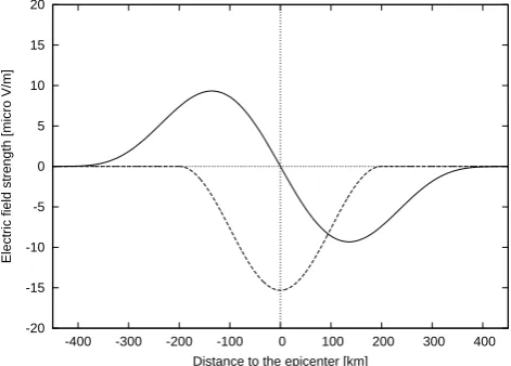
Fig. 3. Vertical electric field at the bottom of the ionosphere Ez(x,zup) is compared to the model Ez(x,zup)/10 (Denisenko

et al., 2008) (solid and dashed lines), with maximum values of 9.3 µV m−1and 153 µV m−1, respectively.

where the matrix0and the coefficients are

0=        

λ1n λ2n 0 0 0 0

α1 α2 −α3 −α4 0 0

λ1nα1λ2nα2−λ3nα3−λ4nα4 0 0

0 0 α5 α6 −α7 −α8

0 0 λ3nα5 λ4nα6 −λ5nα7−λ6nα8

0 0 0 0 β1 β2

        ,

α1=exp(λ1nzlow), α2=exp(λ2nzlow), α3=exp(λ3nzlow), α4=exp(λ4nzlow), α5=exp(λ3nzmid), α6=exp(λ4nzmid), α7=exp(λ5nzmid), α8=exp(λ6nzmid), β1=(6Pkn2+σ (zup)λ5n)exp(λ5nzup),

β2=(6Pkn2+σ (zup)λ6n)exp(λ6nzup). (28)

Now the two components of the electric field in the atmo-sphere can be calculated from Eq. (4)

Ex(x,z)= − ∂

∂x8(x,z), (29)

Ez(x,z)= − ∂

∂z8(x,z), (30)

where the potential 8(x,z) is calculated by formulas (Eqs. 22–25). The third componentEy(x,z)=0, since there

is no variation along the y-coordinate.

6 Summary of the main results

0 0.5 1 1.5 2

-400 -300 -200 -100 0 100 200 300 400

Electric field strength [micro V/m]

Distance to the epicenter [km]

Fig. 4. Horizontal electric fieldEx(x,zup)in the night-time

iono-sphere with6P=0.1S(solid line) and6P=1S(dashed line).

0 20 40 60 80

1e-006 1e-005 0.0001 0.001 0.01 0.1 1 10 100 1000

z [km]

Electric field strength [V/m]

Fig. 5. Height distributions of the maximum values for the vertical

electric fieldEz(a/3,z)in this model (solid line) andEz(0,z)in the

model of Denisenko et al. (2008) (dashed line).

The shape of the graphs of the vertical electric field Ez(x,z)is almost independent of the altitude as it can be seen

by comparison of Figs. 3 and 2. TheEz(x,z)distributions at

the ground and at the upper boundary of the atmosphere are plotted in different scales, where the maximum values are equal to 100 V m−1at ground and 9.3 µV m−1atz=zup. The

shape of the graphs of the horizontal electric fieldEx(x,z)

stays also about the same at differentz=const and is shown in Fig. 4. The height distributions ofEx(x,z)andEz(x,z)

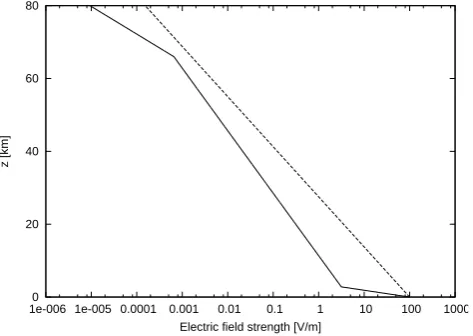
can be presented with their maximal values which are ob-tained atx=0 and x=a/3, respectively. These maximal values are shown in Figs. 5 and 6 as functions ofz.

Since we have chosen a bipolar distribution for the electric field we calculate the penetration into the ionosphere with a

0 20 40 60 80

1e-006 1e-005 0.0001 0.001 0.01 0.1 1 10

z [km]

Electric field strength [V/m]

Fig. 6. Height distributions of the maximum values for the

horizon-tal electric fieldEx(0,z)in this model (solid line) andEx(a,z)in

the model of Denisenko et al. (2008) (dashed line).

characteristic source size dimension ofa=400 km, which is twice the size considered by Denisenko et al. (2008). This is necessary to stay clear that the same total electric field flux,

a Z

0

Ez(x,0)dx, (31)

is going upward from the ground. Such a common parameter is useful for comparison of the results of bipolar and unipolar models.

The horizontal electric field Ex(x,z) at the altitude of

80 km is shown in Fig. 4 and it stays the same in the iono-sphere forz >80 km because of the large field-aligned con-ductivity. It is inverse proportional to the integrated Peder-sen conductivity6P. The typical value of the day-time

iono-spheric Pedersen conductance is about 100 times higher than during night-time. Figure 4 shows the horizontal electric field for night-time conditions with6P=0.1 S. The

maxi-mum value of Ex(x,zup)equals to 1.9 µV m−1. The

day-timeEx(x,z)distribution has almost the same shape, but it

is invisible in this scale because its maximum equals about 0.02 µV m−1.

The electric fields of these magnitudes cannot be observed in the ionosphere because much larger fields of other origin are always present there.

We investigate the relation between the source size dimen-sion and the share of the current which is going up into the ionosphere. For this analysis, we design the current function C which can be derived from the relation

j= ∇ ×C, (32)

that means jx= −∂C

x,km

−100 0 100

z, 100

km

0

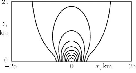
Fig. 7. Current lines for a source size dimension ofa=100 km, where about 30% of the total current is closed inside the atmo-sphere.

jz= ∂C

∂x, (34)

whereC(x,z) is the y-component of the function C which x-, z-components equals zero.

Since an arbitrary constant can be added to C with no change of (Eqs. 33 and 34), we can putC(−b,z)=0. Be-cause of symmetry, we havejx=0 at the vertical linex= −b

as well as atx=b. Therefore, we can integrate (Eq. 33) over zatx= −band obtainC(−b,z)=0. Now we can integrate (Eq. 34) at each levelz=const and construct

C(x,z)=

x Z

−b

jz(x0,z)dx0. (35)

In accordance to Ohm’s law (Eq. 3), the definition of the electric potential (Eq. 4), and the solution for the problem as the Fourier series’s (Eqs. 22–25), we can expressjz(x,z)

as the Fourier series with already known coefficients and in-tegrate each term separately at each levelz=const inside each of three layers in the atmosphere

C1n(x,z)= −σ (z)ω1/ kn, 0≤z < zlow,

C2n(x,z)= −σ (z)ω2/ kn, zlow≤z < zmid,

C3n(x,z)= −σ (z)ω3/ kn, zmid≤z≤zup, (36)

where

ω1= [Anλ1nexp(λ1nz)+Bnλ2nexp(λ2nz)]cos(knx), ω2= [Cnλ3nexp(λ3nz)+Dnλ4nexp(λ4nz)]cos(knx), ω3= [Enλ5nexp(λ5nz)+Fnλ6nexp(λ6nz)]cos(knx).

(37) The resulting current functions are presented in Figs. 7 and 8 for two values of the horizontal scale of the electric field source at ground,a=100 km anda=10 km. These values are typical for a large scale source whose current is closed in the ionosphere and for a small scale source with closure be-ing mainly in the atmosphere. Calculations show that only

x,

km

−

25

0

25

25

z,

km

0

Fig. 8. Current lines for a source size dimension ofa=10 km.

about 3% of the total vertical current is closed inside the atmosphere fora=400 km and about 30% for a=100 km (Fig. 7). For a source size dimension ofa=10 km, the hori-zontal resistivity is much less than the vertical one and only about 20 % of current reaches ionospheric heights (Fig. 8). The total currents are 2×10−7A m−1and 5×10−9A m−1 for a characteristic source size ofa=400 km anda=10 km, respectively. The distance between the current lines in Figs. 7 and 8 are a tenth of the total currents.

In accordance to definition (Eqs. 33 and 34), the lines at whichC(x,z)=const are the current lines for j(x,z). In our model as well as in each two-dimensional model, we define the current function for the layerδy=1 m, and so the current is measured in A m−1instead of Amperes, or we would say that this amount of Amperes exists in aδy=1 m layer.

7 Discussion and conclusion

The values of the horizontal electric fieldEx(x,z)at the

bot-tom of the night-time ionosphere are in the µV m−1 range and about 100 times less during the day. As compared to the results of Denisenko et al. (2008), the electric field penetra-tion from the lithosphere into the ionosphere is much weaker. The maximum value of the vertical component of the electric field at an altitude ofz=80 km is about 15 times less than in the previous model. It can be simply explained by the mod-ification ofσ (z)that is done in this model (see Fig. 1). It can be seen in Fig. 1, thatσ (0)has become ten times less. Since the total electric field flux (Eq. 31) is left about the same, the total current has become 10 times less. This ver-tical current stays approximately the same at all heights in the atmosphere. It can be seen from Fig. 1 thatσ (zup)has

become about 1.6 times larger. The same current would be provided by 1.6 times smallerEz(x,zup), and 10 times less

current by about 16 times lessEz(x,zup). We have just this

result in our new model.

In the model of Denisenko et al. (2008), the horizontal electric fieldEx(x,zup)of about 10 µV m−1penetrating into

times less for the vertical electric field at ground on the same scale. As mentioned above, we have saved the same electric field flux at ground (Eq. 31) and have made ten times less to-tal vertical current. This amount is closed by the ionospheric current. For the same ionospheric integrated conductivity it would be provided by a ten times smallerEx(x,zup). The

previous model was an unipolar distribution and so this cur-rent was divided to both directionsx→ +∞andx→ −∞

in contrast with the only direction from left to right in this model. That is why we obtain here 1.9 µV m−1 nearx=0 instead of±10 µV m−1atx→ ±∞in that model.

In accordance to Ohm’s law, the total vertical electric cur-rent I near ground is equal to the total electric field flux (Eq. 31) multiplied byσ (0). When the horizontal scalea ex-ceeds 100 km, almost the whole currentI goes from ground to the ionosphere as can be seen in Fig. 7, where it is closed. Hence the ionospheric electric current almost equals toI and the appropriateExis aboutI /6P. Therefore, the maximal

value ofExwhich penetrates into the ionosphere is not

sen-sitive to details of the conductivity height distribution defined by the parameters (Eq. 7), and onlyσ (0)is significant when a >100 km. Ifa100 km other parameters (Eq. 7) are im-portant because they define the atmospheric part of the clo-sure current.

Because of the assumption that geomagnetic field lines are parallel in the ionosphere and the field–aligned conductivity is huge, the electric field strength does not vary significantly in higher altitudes.

The main critics is related to the simplified usage of an isotropic electric conductivity. Our approximation for the empirical conductivity profile (Molchanov and Hayakawa, 2008) is rather good as it can be seen from Fig. 1. In the main aim to get analytically solutions, the approximation function is not smooth at the interior boundaries.

As shown in Fig. 5, the vertical electric fieldEzquickly

decreases with height in contrast withExwhich slowly varies

in the higher atmosphere similar to that it stays constant in the ionosphere (see Fig. 6). We think that the parameter of interest in our model, which isEx in the ionosphere, is not

sensitive to the discussed simplification of a real conductivity profile.

However, the conclusion for this model distribution is that the penetration of the electric field of lithospheric origin into the ionosphere is too weak for a measurable result at ionospheric heights, due to the presence of larger electric fields of other nature. The typical magnitude of the elec-tric field in the middle latitude ionosphere is a few mV m−1. To make the maximal value of the ionospheric electric field penetrated from ground equal to 2 mV m−1 instead of ob-tained 2 µV m−1the vertical electric field near ground aught be proportionally larger, 100 kV m−1instead of 100 V m−1, since the model is a linear one. In accordance to Rycroft et al. (2008), such a huge value is never observed. Vershinin et al. (1999) report about electric fields up to 1 kV m−1before strong earthquakes, that is hundred times less than necessary.

The conductivity near ground σ (0)can be in the range 10−14–10−13S m−1 as it is shown in the handbook by Campen et al. (1960). The last value ofσ (0)induces that the electric field in the ionosphere is about ten times larger than in the actual model. It is comparable to the model by Denisenko et al. (2008) and corresponds to the absence of the near ground layer with low conductivity in that model as it can be seen in Fig. 1. Hence, 10 kV m−1vertical elec-tric field above ground would be enough to produce a few mV m−1horizontal electric field in the ionosphere.

Of course this does not mean that no other physical pro-cesses can produce earthquake precursors in the ionosphere. For example, Molchanov et al. (1995) have shown that elec-tromagnetic waves in the frequency range 10−2 to 102Hz can penetrate from ground to the magnetosphere as Alfv´en waves, which can be observed by satellites.

In future investigations, it is necessary to include the nar-rowness of the fault area in the y-direction as well as to vide a better approximation of the realistic conductivity pro-file in the atmosphere. This will require a numerical method to solve the boundary value problem for the electric potential in contrast to pure analytics as done here, which makes this model well suitable for verification. The anisotropic conduc-tivity tensor at ionospheric heights also aught be taken into account, as it was discussed by Denisenko et al. (2008) as well as the role of inclination of the magnetic field lines.

Acknowledgements. This work is supported by grants 07–05–

00135, 09–06–91000 from the Russian Foundation for Basic Re-search and by the Program 16.3 of the Russian Academy of Sci-ences. Additional support is due to the Austrian “Fonds zur F¨orderung der wissenschaftlichen Forschung” under Project I193– N16 and the “Verwaltungsstelle f¨ur Auslandsbeziehungen” of the Austrian Academy of Sciences.

The authors are grateful to the referees whose comments helped considerably to improve the paper.

Topical Editor K. Kauristie thanks two anonymous referees for their help in evaluating this paper.

References

Berthelier, J. J., Godefroy, M., Leblanc, F., Malingre, M., Men-vielle, M., Lagoutte, D., Brochot, J. Y., Colin, F., Elie, F., Legen-dre, C., Zamora, P., Benoist, D., Chapuis, Y., Artru, J., and Pfaff, R.: ICE, the electric field experiment on DEMETER, Planet. Space Sci., 54, 456–471, 2006.

Boyarchuk, K. A., Lomonosov, A. M., Pulinets, S. A., and Hegai, V. V.: Variability of Earth’s atmospheric electric field and ion– aerosols kinetics in the troposphere, Studia Geophysicae et Geo-daetica, 42, 197–210, 1998.

Campen, C. F., Ripley, W. S., Cole, A. E., Sissenwine, N., Condron, T. P., and Solomon, I.: Handbook of Geophysics, The Macmillan Company, New York, 1960.

1009–1017, 2008,

http://www.nat-hazards-earth-syst-sci.net/8/1009/2008/. Debuev, V. and Zelenova, T.: Electron density profile changes in a

pre–earthquake period, Adv. Space Res., 18(6), 115–118, 1996. Gokhberg, M. B., Gufel’d, I. L., Gershenzon, N. I., and Pilipenko,

V. A.: Electromagnetic effects during rupture of the Earth’s crust, Izvestiya Russian Academy of Sciences, Phys. Solid Earth, 21, 52–63, 1985.

Gokhberg, M. B., Pilipenko, V. A., and Pokhotelov, O. A.: Seis-mic precursors in the ionosphere, Izvestiya Russian Academy of Sciences, Phys. Solid Earth, 19(10), 762–765, 1983.

Hargreaves, J. K.: The upper atmosphere and Solar-Terrestrial rela-tions, Van Nostrand Reinold Co. Ltd, NY, 1979.

Kelley, M. C., Livingston, R., and McCready, M.: Large amplitude thermospheric oscillations induced by an earthquake, Geophys. Res. Lett., 12, 577–580, 1985.

Kim, V. P., Khegaj, V. V., and Nikiforova, L. I.: On a possible dis-tortion of the nighttime ionopheric E-region above large-scale tectonic fault, Phys. Solid Earth, 31(7), 580–584, 1996. Kim, V. P., Hegaj, V. V., and Illich-Switych, P. V.: On the

possibil-ity of a metallic ion layer forming in the E-region of the night midlatitude ionosphere before great earthquakes, Geomagnetism and Aeronomy, 33, 658–662, 1994.

Kingsley, S. P.: On the possibilities for detecting radio emissions from earthquakes, Il Nuovo Cimento, 12, 117–120, 1989. Kondo, G.: The variation of the atmospheric electric field at the time

of earthquake, Memoirs of the Kakioka Magnetic Observatory, 13, 11–23, 1968.

Liu, J. Y., Chuo, Y. J., Shan, S. J., Tsai, Y. B., Chen, Y. I., Pulinets, S. A., and Yu, S. B.: Pre-earthquake ionospheric anomalies reg-istered by continuous GPS TEC measurements, Ann. Geophys., 22, 1585–1593, 2004,

http://www.ann-geophys.net/22/1585/2004/.

Molchanov, O. and Hayakawa, M.: Seismoelectromagnetics and re-lated phenomena: History and latest results, Terrapub, Tokyo, Appendixes 9, 10, 2008.

Molchanov, O. A. and Hayakawa, M.: Generation of ULF electro-magnetic emissions by microfracturing, Geophys. Res. Lett., 22, 3091–3094, 1995.

Molchanov, O. A., Hayakawa, M., and Rafalsky, V. A.: Penetra-tion characteristics of electromagnetic emissions from an under-ground seismic source into the atmosphere, ionosphere and mag-netosphere, J. Geophys. Res., 100(A2), 1691–1712, 1995. Molchanov, O., Fedorov, E., Schekotov, A., Gordeev, E., Chebrov,

V., Surkov, V., Rozhnoi, A., Andreevsky, S., Iudin, D., Yunga, S., Lutikov, A., Hayakawa, M., and Biagi, P. F.: Lithosphere-atmosphere-ionosphere coupling as governing mechanism for preseismic short-term events in atmosphere and ionosphere, Nat. Hazards Earth Syst. Sci., 4, 757–767, 2004,

http://www.nat-hazards-earth-syst-sci.net/4/757/2004/.

Park, C. G. and Dejnakarintra, M.: Penetration of thundercloud electric fields into the ionosphere and magnetosphere, 1. Middle and auroral latitudes, J. Geophys. Res., 84, 960–964, 1973. Pogorel’tsev, A. I.: Disturbances of electric and magnetic fields

in-duced by the interaction of atmospheric waves with the iono-spheric plasma, Geomagnetism and Aeronomy, 29, 286–292, 1989 (in Russian).

Pulinets, S. A. and Boyarchuk, K.: Ionospheric precursors of earth-quakes, Berlin Heidelberg New York: Springer, 2004.

Pulinets, S. A., Legen’ka, A. D., Gaivoronskaya, T. V., and Depuev, V. Kh.: Main phenomenological features of ionospheric precur-sors of strong earthquakes, J. Atmos. Solar-Terr. Phys., 65, 1337– 1347, 2003.

Pulinets, S. A., Boyarchuk, K. A., Hegai, V. V., Kim, V. P., and Lomonosov, A. M.: Quasielectrostatic model of atmosphere-thermosphere-ionosphere coupling, Adv. Space Res., 26, 1209– 1218, 2000.

Pulinets, S. A., Hegai, V. V., Kim, V. P., and Depuev, V. Kh.: Un-usual longitude modification of the night-time mid-latitude F2 region ionosphere in July 1980 over the array of tectonic faults in the Andes area: Observations and interpretation, Geophys. Res. Lett., 25, 4133–4136, 1998.

Ruzhin, Yu. Ya. and Depueva, A. Kh.: Seismoprecursors in space as plasma and wave anomalies, J. Atmos. Electr., 16, 271–288, 1996.

Rycroft, M. J., Harrison, G. R., Nicoll, K. A., and Mareev, E. A.: An overview of Earth’s global electric circuit and atmospheric conductivity, Space Sci. Rev., 137, 683–105, 2008.

Sharma, D. K., Rai, J., Chand, R., and Israil, M.: Effect of seismic activities on ion temperature in the F2 region of the ionosphere, Atm´osfera, 19, 1–7, 2006.

Silina, A. S., Liperovskaya, E. V., Liperovsky, V. A., and Meister, C.-V.: Ionospheric phenomena before strong earthquakes, Nat. Hazards Earth Syst. Sci., 1, 113–118, 2001,

http://www.nat-hazards-earth-syst-sci.net/1/113/2001/.

Sorokin, V. M., Chmyrev, V. M., and Yaschenko, A. K.: Electro-dynamic model of the lower atmosphere and the ionosphere cou-pling, J. Atmos. Solar-Terr. Phys., 63, 1681–1691, 2001. Vershinin, E. F., Buzevich, A. V., Yumoto, K., Saita, K., and