Origin of the turbulent spectra in the high-altitude cusp: Cluster spacecraft observations

Origin of the turbulent spectra in the high-altitude cusp: Cluster

spacecraft observations

K. Nykyri1, B. Grison2, P. J. Cargill1, B. Lavraud3, E. Lucek1, I. Dandouras4, A. Balogh1, N. Cornilleau-Wehrlin2, and H. R`eme4

1_{The Blackett Laboratory, Imperial College, London, UK}

2_{CETP/CNRS-UVSQ, 10/12 Avenue de l Europe, 78140, Velizy, France} 3_{Los Alamos National Laboratory, Los Alamos, NM, USA}

4_{Centre d’Etude Spatiale des Rayonnements,31028 Toulouse Cedex 4, France}

Received: 1 August 2005 – Revised: 21 February 2006 – Accepted: 28 March 2006 – Published: 19 May 2006

Abstract. High-resolution magnetic field data from Clus-ter Flux Gate MagnetomeClus-ter (FGM) and the Spatio-Temporal Analysis of Field Fluctuations (STAFF) instruments are used to study turbulent magnetic field fluctuations during the high-altitude cusp crossing on 17 March 2001. Despite the quiet solar wind conditions, the cusp was filled with magnetic field turbulence whose power correlates with the field-aligned ion plasma flux. The magnetic field wave spectra shows power law behavior with both double and single slopes with break in the spectra usually occurring in the vicinity of the local ion cyclotron frequency. Strong peaks in the wave power close to local ion cyclotron frequency were sometimes ob-served, with secondary peaks at higher harmonics indicative of resonant processes between protons and the waves. We show that the observed spectral break point may be caused partly by damping of obliquely propagating kinetic Alfv´en (KAW) waves and partly by cyclotron damping of ion cy-clotron waves.

Keywords. Magnetospheric physics (Magnetopause, cusp and boundary layers; Plasma waves and instabilities) – Space plasma physics (Nonlinear phenomena; turbulence)

1 Introduction

The high-altitude cusps are regions where the magnetosheath plasma has the most direct access to the ionosphere, and their structure is determined by a complex interaction between the shocked solar wind and the geomagnetic field. The cusps are also a region of significant turbulence which can be created by solar wind (bowshock) perturbations, magnetic reconnec-tion or intrinsic instabilities present in the cusp. Prior to the mid-1990s, in situ measurements of the cusp were relatively infrequent, although important results came from the HEOS

Correspondence to: K. Nykyri

([email protected])

and Hawkeye missions (e.g. Paschmann et al., 1976; Kessel et al., 1996; Dunlop et al., 2000). The recent Polar and In-terball missions have been important in illuminating many examples of cusp physics. Of particular interest for this pa-per has been the identification of lobe reconnection (Scudder et al., 2002; Fuselier et al., 2000; Russell et al., 2000), the spatial extent of the cusp (Zhou et al., 1999, 2000) and in-situ magnetic field turbulence (Savin et al., 1998; Chen and Fritz, 1998; Le et al., 2001; Savin et al., 2002, 2004).

The four spacecraft, multi-instrument Cluster mission rep-resents the first of a new generation of magnetospheric physics missions, and is ideal for studying the high- and mid-altitude cusps. Cluster has revealed for the first time many important aspects of the structure of the high-altitude cusps, and especially how they are related to the prevail-ing solar wind conditions (e.g. Lavraud and Cargill, 2005; Cargill et al., 2005; Lavraud et al., 2005). In particular, it is becoming apparent that the orientation of the Interplanetary Magnetic Field (IMF) plays a pivotal role. For Northward IMF, a picture is emerging of a cusp influenced by lobe re-connection (Vontrat-Reberac et al., 2003; Twitty et al., 2004) with Earthward-directed plasma jets being observed, but also containing regions of stagnant plasma (Lavraud et al., 2002, 2004). On the other hand, for Southward IMF, the cusp is dominated by tailward convection due to sub-solar reconnec-tion (Cargill et al., 2004).

Le et al., 2001). The waves show no significant correla-tion between the spacecraft when the inter-spacecraft sepa-ration is either 600 or 100 km (Nykyri et al., 2003). It is un-clear whether these waves are generated in-situ by the plasma flows, or whether they are convected from remote reconnec-tion sites at the lobes. Since the reconnecreconnec-tion site would be severalRE away, this implies a damping time longer than

300 s for flows of 100 km/s. A recent study by Sundkvist et al. (2005) is implying a local generation mechanism for these waves: they observe that the Poyinting flux is changing direction at the proton gyrofrequency.

Our previous studies (Nykyri et al., 2003, 2004) were car-ried out using magnetic field data from the Flux Gate Magne-tometer (FGM) instruments on Cluster (Balogh et al., 2001), and focused on the frequency range between 0.1 Hz to over 1 Hz. For these examples, the proton cyclotron frequency (fI C) was in the range 0.7–1.5 Hz. We found indications of

wave power at higher cyclotron harmonics, and the transi-tion to a different turbulence regime above fI C. The

lat-ter possibility has also been discussed by Sundkvist et al. (2005), who suggest that the cusp waves belong to the kinetic Alfv´en branch below the proton cyclotron frequency and are electromagnetic ion-Bernstein waves above that frequency. This is also confirmed by Grison et al. (2005) who used the

k-filtering technique, and showed that kinetic Alfv´en waves dominate the electromagnetic spectrum up to 1Hz and above 0.8 Hz intense Bernstein waves are observed.

A limitation of our earlier studies was the level of in-strument noise above a few Hz and so this paper returns to the topic of cusp turbulence by examining magnetic field turbulence at frequencies up to 10 Hz using measurements from the Cluster Spatio-Temporal Analysis of Field Fluctu-ation (STAFF) experiment (Cornilleau-Wehrlin et al., 1997; Cornilleau-Wehrlin et al., 2003) as well as from FGM. The main objective in using the two instruments is to get a contin-uous spectra from lower (FGM) to higher (STAFF) frequen-cies which enables us to study spectral structure both below and above the local ion cyclotron frequency (fI C).

We return in this paper to the well-studied high-altitude cusp crossing on 17 March 2001 (Vontrat-Reberac et al., 2003; Nykyri et al., 2003, 2004). Section 2 presents the rele-vant instrumentation and cusp overview, Sect. 3 the analysis techniques, Sect. 4 the measurements and Sects. 5 and 6 our interpretation of the observed spectral structure in terms of wave damping.

2 Instrumentation and overview of cusp

We use data from three instruments on-board Cluster. High resolution (22.4 vectors/s) magnetic field measurements are obtained from the Flux Gate Magnetometer (FGM: Balogh et al., 1997, 2001) from all four spacecraft. FGM data provides the overall cusp magnetic field context, and wave power at frequencies up to 3 Hz can be accurately calculated.

Search coil magnetometers (STAFF: Spatio-Temporal Anal-ysis of Field Fluctuation experiment: Cornilleau-Wehrlin et al., 2003; Cornilleau-Wehrlin et al., 1997) on-board all four spacecraft are used to calculate wave power from 1 Hz up to 10 Hz. Ion plasma measurements are obtained using the Cluster Ion Spectrometry (CIS: R`eme et al., 2001) ex-periment and are essential for providing the plasma context. Data from the Hot Ion Analyser (HIA) instrument on-board spacecraft 1 and 3 and the ion COmposition and DIstribu-tion FuncDIstribu-tion analyser (CODIF) instrument on-board space-craft 4 are used. The plasma velocity moments are avail-able every∼4 s from spacecraft 1 and 4 and every 12 s from spacecraft 3.

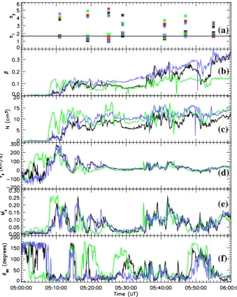
The cusp crossing chosen occurs on an outbound orbit be-tween 05:00 and 07:00 UT on 17 March 2001. This interval has been extensively studied (Vontrat-Reberac et al., 2003; Nykyri et al., 2003, 2004), so that the overall phenomenology is well established. Figure 1 shows the power spectral slopes (discussed later in Sects. 4.3 and 4.4) and plasma parameters measured by spacecraft 1, 3 and 4 between 05:00–06:00 UT. The color code used in this paper is as follows: black, red, green and blue correspond to spacecraft 1, 2, 3 and 4 respec-tively (referred to hereafter as sc1, sc2, sc3, sc4). Panels b-f show the ion beta (β), plasma density (N), parallel plasma velocity (Vk), Alfv´en Mach number (MA) and the angle

be-tween plasma flow and the magnetic field (θBV). The

space-craft separation is 600 km and Cluster altitude in the cusp is ∼ZGSM=8RE.

The spacecraft leave the magnetosphere shortly after 05:00 UT, and cusp entry can be seen first as an enhanced density at sc3 (Fig. 1c). Between 05:07 and 05:13 UT, the spacecraft sequentially entered the cusp, a region charac-terized here by a density of a few particles cm−3 with an Earthward-directed plasma flow of approximately 250 km/s (Fig. 1d), although this value varies between the spacecraft.

Cluster remains in the cusp from approximately 05:13 to 06:20 UT, and during this time the flows decline to almost zero. However, this decline masks considerable structure, with strong velocity shears being present over timescales of a few minutes. Between 05:00–06:00 UT the magnetic field gradually decreases (not shown) from∼100 nT to 45 nT, im-plying proton cyclotron frequencies of 1.5–0.7 Hz. In this paper we only focus on data up to 06:00 UT.

The solar wind conditions (not shown) are obtained from Advanced Composition Explorer (ACE) spacecraft at the L1 point (a lag time was applied assuming 285 km/s solar wind speed). During the interval of 04:30–06:30 UT solar wind had a magnetic field magnitude of approximately 5 nT,Bz

was mostly pointing northward (except for a brief southward turning at about 05:40 UT), with a magnitude of approxi-mately 3 nT.Bywas mostly positive with a magnitude of 3 nT

but turned negative at about 05:17 UT for about 35 min. Bx

(a)

(b)

(c)

(d)

(e)

(f)

Fig. 1. Power spectral slopes and plasma parameters between 05:00–06:00 UT. Panel (a) shows inertial (s1) and dissipation (s2) range slopes. The solid line is at 5/3. Panels (b)–(f) show the ion plasma beta (β), the plasma density (N), parallel plasma velocity (Vk), Alfv´en Mach

number (MA) and the angle between plasma flow and the magnetic field (θBV). Black is data from spacecraft 1 (hereafter sc1), red from sc2,

green from sc3 and blue from sc4. The spacecraft separation is 600 km and Cluster altitude in the cusp is∼ZGSM=8RE.

In analyzing the magnetic field turbulence we use same temporal demarcation of the cusp as described in Nykyri et al. (2004) who divided the analysis into regions based on the local plasma properties: a strong shear-flow cusp between 05:07 and 05:25; a stagnant cusp between 05:25 and 05:35 and a moderate shear-flow cusp between 05:35 and 05:56.

3 Analysis methods of cusp magnetic field fluctuations

We evaluated the total power of the magnetic field fluctu-ations between 05:00–06:00 UT using data from both the

STAFF and FGM instruments. The magnetic field time series was examined and the short duration data gaps were linearly interpolated. Before evaluating the Fast Fourier Transform (FFT) for each interval, a Hanning window was applied to the de-trended data set. The total power is then the trace of the power spectral matrix:Pt ot=Px+Py+Pz.

3.1 Combining STAFF and FGM: waves close to the ion cyclotron frequency

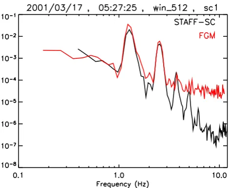
Fig. 2. Total power of magnetic field fluctuations observed by

Clus-ter FGM (red) and STAFF (black) instrument on-board of space-craft 1 centered at 05:27:25 UT (2×256 data points are used).

overlap region (∼0.5–2 Hz) both instruments measure the same power. For this purpose 512 point windows (∼22.9 s) were used at each interval of the comparison study in Sect. 4.3.

As an example of how FGM and STAFF data can be com-bined, we first look at the strong spectral peaks near the ion cyclotron frequency and its harmonics when the spacecraft are in the stagnant cusp. Examination of the magnetic field time series shows that the several small amplitude (∼1–2 nT) wave trains were observable at all four spacecraft between ∼05:25–05:29 UT and between∼05:45–05:49 UT, showing no correlation between the spacecraft pairs (see Nykyri et al. (2004) for more details).

Figure 2 shows the total power in the magnetic field fluc-tuations centered at 05:27:25 UT (for each instrument the data is averaged over 2 windows of 256 points) measured by FGM (red) and STAFF (black) on spacecraft 1. It is clear that between 0.5–2.8 Hz, the power from both instruments are in good agreement. The frequency corresponding to the dominant peak is about 1.1 times the local ion cyclotron fre-quency. The first harmonic of the fundamental frequency is also observable from both FGM and STAFF. Because of the better sensitivity at higher frequencies, STAFF can also de-tect the 2nd, 3rd and 4th harmonics (see also Cargill et al., 2005).

Thus, both instruments measure the same peak of the fun-damental frequency where their measurements overlap, so we have confidence in combining their spectra when using longer (approximately 6.1 min) intervals.

3.2 Slope validation

However, longer window sizes have better statistics and are used to evaluate the slope of the power spectra (Sect. 4.3). There we use∼6.1 min windows for both instruments which corresponds to 8192 points with FGM sampling frequency of 22.4 vectors/s. Because the sampling frequency for STAFF is slightly higher than for FGM, we require more STAFF points to give the same total time interval. However, instead of a single window it is sometimes better to use short but numer-ous windows for STAFF spectra.

The magnetic field power spectra shows a clear break dur-ing some intervals dividdur-ing the spectra in two different power law regimes. We define the frequency at which this dis-persion in spectrum occurs as a break point frequency,fbf.

For each interval, we have visually determined thefbf and

the frequency range of the slope calculation for both instru-ments. FGM data are used below the dispersion breakpoint (typically below 1 Hz) and STAFF-SC above it (up to 10 Hz). We illustrate this point in Fig. 3c (the rest of Fig. 3 will be discussed fully in Sect. 4.3), which shows the total power of magnetic field fluctuations measured by sc3 from FGM (red) and STAFF (black) instrument at an interval centered at 05:19 UT. The breakpoint is visually determined to be at 1 Hz which is indicated by a black vertical line. During this interval the FGM data is used in slope calculation between 0.015–0.15 Hz and STAFF data is used between 3-10 Hz. It can be seen that both instruments agree between 0.6–3 Hz.

In addition to these studies, the slopes have been evaluated over a common range of frequencies (between 0.5 and 2 Hz) from both instruments. These slopes do not have a phys-ical meaning but they indicate that the spectral breaks are not an instrumental effect. Table 1 contains a comparison of the slopes estimated from STAFF and FGM in the frequency range [0.5, 2Hz] for intervals centered at 05:41:00 UT. The comparison of the results obtained from one large-window FFT and the mean of many short windows cannot be made when spectral peaks are detected because of the number of frequencies present in the peak (512 point windows have a low resolution in frequency). So, the comparison has been performed during an interval that displays no peaks, and where almost no spectral break is detected (see Fig. 14a, which will be fully explained in Sect. 6).

(b)

(d)

(a)

(c)

Fig. 3. The power spectrum of magnetic field fluctuations observed by Cluster FGM (red) and STAFF (black) instrument at interval centered

at 05:19 UT by sc1 (a), sc2 (b), sc3 (c), and sc4 (d). Power law slopes are shown above the spectra, and their methods of evaluation are discussed fully in the text. The spectral breakpoint is marked with black vertical line and localfI Cwith purple arrow.

Thus the agreement between slope measurements from FGM and STAFF data during the same time interval and in the same frequency range ensure us that the spectral breaks do not originate from instrumental artifact but have a physi-cal meaning.

3.3 Stationarity of the time series

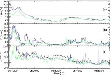
In order to assess the stationarity of the time series, we have computed the variance of the plasma velocity field at each spacecraft for the same time intervals as the slope calcula-tion. Figure 4a shows the velocity field variance using a ∼6.1-min window and the total plasma velocity measured by sc1, sc3 and sc4 is shown in Fig. 4b. The variance is less than 45 km/s for all the intervals after 05:17 UT, which is less than 10% of the local Alfv´en speed (Fig. 2c). Be-cause the Alfv´en/ion cyclotron modes have phase speeds of vph=vAcosθkB, where θkB is the angle of propagation

with respect to magnetic field, for most cases the waves will

Table 1. Slopes of power spectra between [0.5–2 Hz] at 5:41:00 UT.

FGM STAFF FGM-STAFF gaps (8192 pts.) (9216 pts.)

Sc1 –3.18 –3.32 0.14 none Sc2 –2.46 –3.93 1.47 many Sc3 –2.38 –2.53 0.15 small Sc4 –2.6 –3.89 1.29 small

FGM STAFF FGM–STAFF gaps (8192 pts.) (18×512 pts.)

(a)

(b)

(c)

Fig. 4. Variance (σ) of the plasma velocity shown (a) during each∼6.1-min interval used in the power spectral slope calculations. The total plasma velocity (b) and the Alfv´en speed (c) measured by sc1, sc3 and sc4 between 05:00–06:00 UT are shown.

(a)

(b)

Fig. 5. Panel (a) shows the total integrated power in the magnetic field fluctuations observed by the FGM instruments on all four spacecraft

between 05:00–06:00 UT. The frequency range is 0.06 Hz–3 Hz and a 2048 point window shifted with a 4-s increment is used). Panel (b) shows the total ion plasma number flux measured by sc1, sc3 and sc4.

propagate faster than the flows, and the intervals centered af-ter 05:17 UT may be considered reasonably steady.

In addition to the intervals used in the comparison study we have also evaluated FGM spectra with 1024, 2048, 4096, and 16 384 points corresponding to 45.4, 90.7, 182.9 and 731.5 s, respectively. Although there are intervals before 05:17 UT where the variance is less than 45 km/s using the 90.7-s interval, errors in the power law indices increase for

(a)

(b)

Fig. 6. The ratio of the integrated perpendicular and parallel (with respect to the magnetic field) power,P⊥/P||, at the inertial range (a)

between 0.015 Hz–fbf and at the range betweenfbf–3.0 Hz (b). Calculations use 8192 point window shifted by 1-min increments over

FGM data.

4 Observations

4.1 Total integrated power of magnetic field fluctuations To set our investigation in context, we present the time his-tory of the magnetic field fluctuations. Figure 5a shows the integrated power in magnetic field fluctuations between 05:00 and 06:00 UT measured by FGM with a 2048 point window (∼93.1 s) sequentially shifted with a 4-s increments through the cusp. The integration is performed over a fre-quency range of 0.06 Hz–3 Hz (The upper limit of 3 Hz is chosen to avoid the lower sensitivity of FGM at higher fre-quencies). Figure 5b shows the ion number flux,f=nvt ot,

(or ion currentJi/q) measured by sc1, sc3 and sc4. One can

see that the integrated power of the magnetic field fluctua-tions correlates well with the ion number flux. (Grison et al. (2005); Sundkvist et al. (2005) also show the correlation be-tween wave activity and field-aligned ion fluxes). This is es-pecially clear at cusp entry∼05:07:30 UT, where sc1 and sc4 measure a low flux while also seeing a low level of magnetic field fluctuations, while sc3 sees an increased flux. The total plasma velocity (see Fig. 4b) and field-aligned plasma veloc-ity (see Fig. 1d) at cusp entry is similar for all 3 spacecraft but sc3 sees an enhanced plasma density (Fig. 1c) compared to other two which results in enhanced plasma number flux. When the flow and number flux vanish before 05:30 UT, so does much of the power in the waves (see Fig. 2. and also Cargill et al. (2005); Grison et al. (2005)). Smaller scale ve-locity fluctuations re-appear at about 05:35 UT and persist throughout the rest of the interval.

4.2 Transverse vs. compressional fluctuations

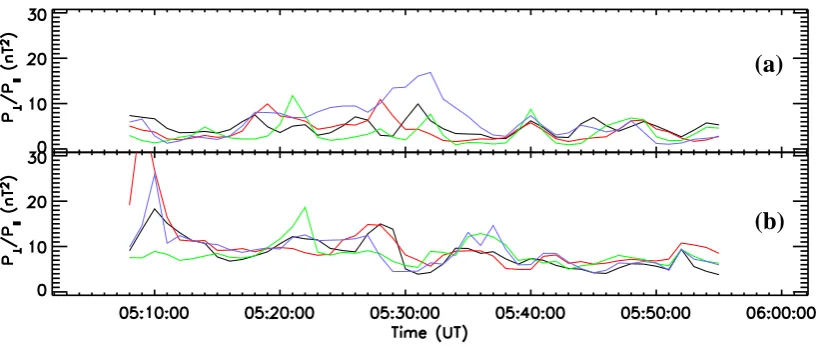
Using FGM data we have evaluated the ratio of the perpen-dicular and parallel (with respect to the ambient magnetic

field) wave power, P⊥/P||, whereP⊥=Pt ot−P|| andP|| is

the power in mean field (|b|) fluctuations. Figure 6 shows the ratio of the integrated perpendicular and parallel wave power,P⊥/P||between 0.015 Hz and break frequency (fbf)

(a), and betweenfbf and 3.0 Hz (b). An 8192 point window

slided with 1-min increments through the data set between 05:00–06:00 UT is used. In both ranges the fluctuations are mostly transverse.

4.3 Calculation of power spectral indices below and above spectral breakpoint

We have evaluated the power spectra obtained from FGM and STAFF data from all four spacecraft using∼6.1-min in-tervals, centered at seven different times: 05:11 (cusp entry) (However, we note that this interval has a problem of sta-tionarity as described in Sect. 3.3), 05:19 (shear-flow cusp), 05:25 (stagnant cusp boundary), 05:29 (stagnant cusp), 05:41 (moderate shear flow cusp), 05:47 (stagnant cusp boundary) and 05:55 UT (moderate shear flow cusp). In this section we first discuss in detail one of the seven periods, that centered at 05:19 UT, then review the others.

has the same –5/3 power law in the inertial range as a high Reynolds number fluid (Kolmogoroff, 1941). In the solar wind the plasma flow speed is much larger than the typical wave speed (VSWVphase), so that a time series can be

inter-preted as a 1-D spatial cut, enabling a transition from the fre-quency space to the wave number (k) space. However, in the high-altitude cusp (and for the presented crossing) the Alfv´en speed and thus the phase speed of the waves is much larger than the plasma flow speed (VphaseV), so that one cannot

do a direct transition fromf-space to thek-space. The mag-netic field power spectrum is thus likely to be dominated by propagating temporal fluctuations (waves) from the different sources. In the regions of enhanced flows the frequency of these waves is Doppler-shifted according to

fSC=

1

2π(V kcos(θkV)+ω) , (1)

where k is the wavenumber andθkV is the angle between

thek-vector and the plasma velocity. It is also possible that some Doppler shifted spatial structures are present. In Sect. 5 we will discuss possible interpretations for this double sloped spectra. However, for simplicity we will refer hereafter to the spectra below the spectral breakpoint (usually atfI C) as an

“inertial” range and above as a “dissipation” range, although they cannot be directly compared with the existing turbulent theories of the solar wind.

The frequency ranges used in the slope calculations in the inertial and dissipation ranges are visually determined based on the shape of the spectra. During this interval the upper frequency limit for the inertial range is below 0.2 Hz which gives slopes of –1.12, –1.25, –1.66 and –1.31 with error-bars of 25 %, 24%, 15%, and 32 % for sc1, sc2, sc3 and sc4, respectively. Here the spacecraft separation is 600 km and we did not observe any correlation of the magnetic field time series between different spacecraft pair. Therefore we cannot apply thek-filtering technique (Sahraoui et al., 2003; Grison et al., 2005) (which works if the wave length of the waves is larger than the spacecraft separation) to do a transition from the frequency space to thek-space.

The slopes calculated from STAFF data above 1 Hz are much steeper and for this time interval vary between –4.9 and –4.1, such slopes being characteristic of a turbulent dis-sipation range (see (Goldstein et al., 1994) for a discussion of this in the solar wind). In each case, the spectral break-point of∼1 Hz is slightly below the local proton cyclotron frequency, which is marked with purple arrow in Fig. 3.

This analysis can be extended to other intervals with the aim of investigating whether there is any connection between the values of the indices and the local plasma properties, es-pecially the velocity. Figure 1a shows the magnitudes of iner-tial,s1, (squares) and dissipation range,s2, (stars) power law slopes with the associated error bars (these are smaller than the size of the square) during the seven intervals described in the beginning of this section.

Figure 13a shows the magnitudes of inertial range slopes with error bars (the range of slope calculation is visually de-termined for each interval) dede-termined from the FGM for each minute through the cusp. The solid, horizontal line is at 5/3, and the solid wavy line marks the average slope value of all four spacecraft at each interval. There are significant differences between different times, and between different spacecraft at the same time.

When considering all intervals, the inertial range slopes vary from –1.0 to –2.7. In the dissipation range, we find slopes between –2.9 and –5.2. The exact frequency range for slope calculation for both instruments is determined individ-ually for each spacecraft based on the shape of the spectra as explained in Sect. 3.2.

4.4 Comparison of spectral indices with the plasma param-eters

As Cluster moves through the cusp, not only do the plasma parameters change, but so does the background magnetic field. The local Alfv´en speed decreases from about 800 km/s to 350 km/s between 05:13 and 06:00 UT (see Fig. 4c) and during each 6.1-min interval Cluster moves approximately 1100 km in a Sunward direction. After 05:12 UT the ion tem-perature (not shown) is almost constant at all four spacecraft, and the density increases as shown in Fig. 1c, albeit with fluctuations. In order to compare the plasma parameters with spectral indices at each interval we have calculated∼6.1-min averages of the plasma parameters, their maximum and min-imum value and the difference between these maxmin-imum and minimum value during each interval (this is done for those parameters shown in Fig. 1 but also for others such as per-pendicular velocity, parallel number flux, total number flux, perpendicular number flux, temperature, plasma pressure and total pressure). No correlation with the power spectral slopes was found in either inertial or dissipation ranges.

4.5 Ion distribution functions and plasma velocity during wave observations

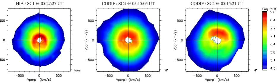
Fig. 7. Ion distribution functions in parallel/perpendicular-plane (from HIA-instrument) at 05:27:27 UT (a). Proton distribution functions

(from CODIF-instrument) at sc4 (at 05:15:01 UT (b) and at 05:15:21 UT (c)), respectively.

2003) and to the electromagnetic ion cyclotron waves (Sund-kvist et al., 2005). Figure 7a of Nykyri et al. (2004) shows that sc4 also observes waves close to the ion cyclotron fre-quency between 05:15:29–5:15:41 UT, but only the funda-mental peak is clear (with FGM) and the waves do not form as regular wave train as at ∼05:27:27 UT. The STAFF bx

spectra at sc4 between 05:15:35–05:15:45 UT shows two peaks: one at the cyclotron frequency at≈1.3 Hz and other at ≈3 Hz, so that the second peak is not a harmonic. Prior to this interval sc4 observes an isotropic distribution at 05:15:05 UT (Fig. 7b) corresponding to a diminished field-aligned flow (Fig. 1d). There is also an extensive literature concerning the generation of IC waves due to instabilities in plasma flows, especially for ionospheric parameters (e.g. Kindel and Ken-nel, 1971; Penano and Ganguli, 2002). For field-aligned flow (such as we mostly detect here (see Fig. 1d and 1f), only electrostatic calculations have been carried out, but they sug-gest that waves can be excited at many harmonics of thei

(Gavrishchaka et al., 2000; Ganguli et al., 2002). However, electrostatic is just a limiting case. Because the ion cyclotron perturbations are two dimensional they will always be asso-ciated with current and hence magnetic fluctuations. Trans-verse flow layers can also become unstable and excite IB waves (Reynolds and Ganguli, 1998).

The diminution of the flow magnitude, especially after 05:25 UT, has two possible explanations. First, the ACE data shows that the IMFBzslightly rotates (and also theBy),

turn-ing negative at about 05:30 UT, so that the amount of the re-connecting flux tailward of the cusp decreases, resulting in a weaker flow. Indeed parallel flows (with a lower magnitude) reappear after the IMF turns northward at about 05:35 UT.

Secondly, Cluster is moving further into the cusp, encoun-tering field lines that have reconnected some time in the past. This can be seen as a more symmetric ion distribution func-tion measured by sc1 at 05:27:27 UT (Fig. 7a). This distribu-tion coincides with the magnetic field observadistribu-tions of the ion cyclotron harmonics at 05:27:14–05:27:37 UT (Fig. 2). One

can notice that the parallel part of the distribution (beam) is slightly enhanced, and in the other direction a small deple-tion can be seen, reminiscent of a small loss cone. The mag-netic hodograms calculated by Nykyri et al. (2004) (Figs. 10 and 13) show that the waves are clearly electromagnetic at ∼05:25–05:29 UT and 05:45–05:49 UT during the observa-tions of the several harmonics. It is presently not clear why the harmonics are not clearly evident during the strongest velocity shear (05:15:21 UT) but favor the regions where plasma has become nearly stagnant (and has small velocity shear 10–40 km/s) and has these more symmetric distribu-tion funcdistribu-tions. However, they are not present in the regions where the plasma has been stagnant for several minutes (i.e. 05:30 UT).

5 The origin of the spectral breakpoint

0 1 2 3 4 5 6 7 8 9 0

1 2

f/fi

0 1 2 3 4 5 6 7 8 9

−0.2 −0.1 0

γ

/f i

0 1 2 3 4 5 6 7 8 9

0 1 2

E/B ((mV/m) /nT)

k₋|(ω

i/vthi)

(a)

(b)

(c)

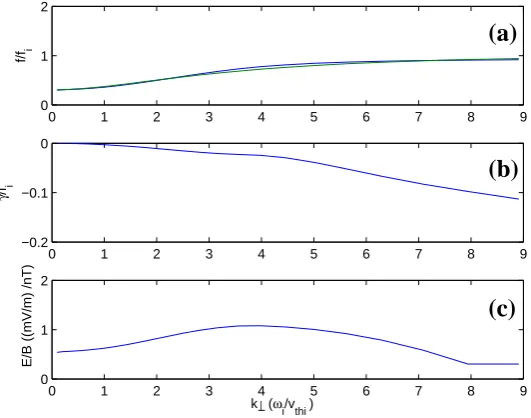
Fig. 8. Solutions from WHAMP code. (a) shows the real frequency of a kinetic Alfv`en wave withkk=0.1 normalized to ion cyclotron

frequency atB=85 nT as a function ofk⊥ (blue). The green line in (a) shows the solution of the real frequency calculated from the

dispersion relation of kinetic Alfv´en (Eq. 2) waves normalized to WHAMP units. (b) Damping (imaginary frequency) as a function ofk⊥.

(c)E⊥/B⊥-ratio.

open solar coronal magnetic field region) by Dmitruk et al. (2004) show the coexistence of discrete modes and turbu-lence in a presence of a strong background magnetic field. It therefore may be possible that both energy cascade and lin-ear modes coexist in the cusp geometry (with magnetic field of 100–60 nT and ion beta of 0.02–0.4).

Here we first consider the possibility that the break point frequency may arise due to fluctuations that cannot be re-supplied by the cascade because they damp too efficiently. In a collisionless plasma there is no dissipation due to col-lisions, but dissipation arises due to wave-particle interac-tions such as Landau and cyclotron damping. Nykyri et al. (2003, 2004) show that the waves were propagating at va-riety of angles with respect to background magnetic field (θkB=0◦–90◦), thus all of parallel, obliquely and

perpen-dicularly propagating waves need to be damped to give a spectral break point. To investigate wave damping in the vicinity of the ion cyclotron frequency, we have used the WHAMP (R¨onnmark, 1982) code with Maxwellian distri-butions with number density ofn=10/cm3and temperatures of 17 eV (0.2 MK) and 170 eV (2.0 MK) for electrons and protons, respectively. These values correspond to measured values by Cluster PEACE and CIS instruments. We run the model with magnetic fields of 85 nT and 60 nT, correspond-ing to different regions in the cusp. There are four wave modes at the vicinity of cyclotron frequency that may be present in the observed spectra: 1) Kinetic Alfv´en waves, 2) Ion cyclotron/Alfv´en waves, 3) Ion Bernstein waves and 4) Fast/magnetosonic waves. In the following we will discuss their importance in determining the breakpoint frequency.

We require that the imaginary frequency exceeds 20% of the real frequency in order to ensure that the particular mode is important contributing to the break frequency. We identify the range of parallel (kk) and perpendicular (k⊥) wave

num-bers andωfor these damped waves and evaluate the Doppler shift for these solutions in the end of this section.

5.1 Damping of the kinetic Alfv´en waves

Kinetic Alfv´en waves (KAW) can be viewed as a coupling of the ion acoustic and shear Alfv´en modes (Lysak and Lotko, 1996). They can exist in a plasma withme/mi≤βe<1. For

this cusp crossing, the ion beta between 05:00–06:00 UT varies between 0.02 and 0.4, and the electron and ion temper-ature ratio,Te/Ti is about 0.1 (this can be determined from

PEACE data), so thatβelies between 0.002 and 0.04 and is

within the required range.

In the limit ofω<ωi, Stasiewicz et al. (2000) derived a

dis-persion relation for KAW including the finite Larmor radius and finite frequency effects:

ω=k||vA

s

1+k2_⊥(r_i2+r2

s)− ω2

ω_i2(1

+k_⊥2r_i2) , (2)

whereri is ion cyclotron radius,ωi is the ion cyclotron

fre-quency,vAis Alfv´en speed, andrs=

q

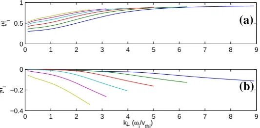
kbTe/(miω_i2).

0 1 2 3 4 5 6 7 8 9 0

0.5

f/fi

0 1 2 3 4 5 6 7 8 9

−0.4 −0.2 0

γ

/fi

k−|(ω_i/v_thi)

(a)

(b)

Fig. 9. Solutions from WHAMP code for kinetic Alfv´en waves. (a) shows the real part and (b) shows the imaginary part of frequency

withkk=0.1 (blue),kk=0.13 (green),kk=0.16 (orange),kk=0.2 (aqua),kk=0.25 (magenta),kk=0.32 (yellow) normalized to ion cyclotron

frequency atB=85 nT as a function ofk⊥.

Table 2. Properties of Kinetic Alfv´en waves (KAW) when damping becomes 20% of the real frequency (calculated from WHAMP model

with Maxwellian electron and proton species withB=85 nT). Columns list parallel and perpendicular wave numbers and wave lengths, real frequency and wave propagation angle with respect to magnetic field. Ion cyclotron radius,rt hi, used here is 22 km.

KAW kk(1/rt hi) k⊥(1/rt hi) λk(km) λ⊥(km) ω/ωi θkB (degrees)

0.32 1.0 432 138 0.67 72 0.25 2.2 553 63 0.78 84 0.2 3.5 691 39 0.85 87

from the dispersion relation matches the WHAMP solution quite nicely withkk=0.1. The wave numbersk⊥andkkare

normalized to the inverse gyroradius, 1/ri=ωi/vt hi.

Fig-ure 8b shows the imaginary part (damping) of the frequency (γ /fi). One can see that damping increases rapidly above k⊥=4 and reaches over 10% of the real frequency atk⊥=7.9.

TheE⊥/B⊥-ratio (shown in Fig. 8c) is of the order of unity

(in units (mV/m)/nT). This is of the order of the Alfv´en speed indicating that the wave is mostly electromagnetic.

Figure 9a is in the same format as Fig. 8a, but in addi-tion to soluaddi-tion withkk=0.1 (blue), WHAMP solutions with kk=0.13 (green), kk=0.16 (orange), kk=0.2 (aqua), kk=0.25

(magenta) andkk=0.32 (yellow) are shown. Panel (b) shows

that damping becomes more important askkincreases.

Let us consider the following physical argument that de-termines the values ofk⊥ at which dissipation of KAW

be-comes significant. Hasegawa and Chen (1976) state that in the collisionless regime if β>(<)0.1, ion (electron) Lan-dau damping dominates the dissipation of the KAW. Here the ion beta varies between 0.02–0.4 so it is likely that ei-ther damping mechanism may occur in different regions of the cusp. Let us first consider electron Landau damping. By neglecting the finite frequency effects in Eq. (2), it can be shown that whenω/ kk=VA

q

1+(1+Te/Ti)k⊥2ri2≈Vt he,

(where the electron thermal speed, Vt he=

q

βiTemi

2TimeVA), the

dissipation becomes significant for k⊥≈(1−6)/ri

(corre-sponding toβi=0.02−0.4). The maximum heating rate for

ions due to the ion Landau damping is obtained withk⊥ri=1

(Hasegawa and Chen, 1976).

Table 2 lists the properties of the KAW when damping becomes 20% of the real frequency. Only solutions with

kk>0.19 have damping rates exceeding 20% of the real

fre-quency. Calculations of the Doppler shifted theoretical spec-tral breakpoint frequencies of the KAW waves in Fig. 13c (Fig. 13 will be fully discussed at the end of this section) use these values forkk,k⊥,ω, andθkB. It can be seen that

damping of the obliquely propagating (θkB=72–87◦) KAW

can lead to the observed spectral breakpoint frequency. This implies parallel wave lengths of 430–690 km and perpendic-ular wave lengths of 40–140 km (the ion gyroradius used here is 22 km (forTi=2 MK,B=85 nT)). Table 3 is in the same

format as Table 2 showing WHAMP solutions forB=60 nT (ri=31 km). These solutions are very similar to those of

Ta-ble 2.

5.2 Damping of the Alfv´en/ion cyclotron modes

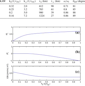
Figure 10 is in the same format as Fig. 8a and shows the real and Fig. 8b imaginary frequencies, and Fig. 8c the

E⊥/B⊥−ratio of ion cyclotron (IC) waves as a function

of kkwithk⊥=0. The damping rate increases significantly

Table 3. Properties of Kinetic Alfv´en waves (KAW) when damping becomes 20% of the real frequency (calculated from WHAMP model

with Maxwellian electron and proton species withB=60 nT). Columns list parallel and perpendicular wave numbers and wave lengths, real frequency and wave propagation angle with respect to magnetic field. Ion cyclotron radius,rt hi, used here is 31 km.

KAW kk(1/rt hi) k⊥(1/rt hi) λk(km) λ⊥(km) ω/ωi θkB (degrees)

0.32 2.0 612 98 0.71 81 0.25 3.2 783 61 0.8 85 0.2 5.0 980 39 0.86 88 0.16 7.2 1224 27 0.86 89

0 0.1 0.2 0.3 0.4 0.5 0.6 0.7 0.8 0.9 1 0

0.5 1

f/fi

0 0.1 0.2 0.3 0.4 0.5 0.6 0.7 0.8 0.9 1 −1

0 1

γ

/fi

0 0.1 0.2 0.3 0.4 0.5 0.6 0.7 0.8 0.9 1 0

0.5 1

E/B ((mV/m) /nT)

k||(ωi/vthi)

(a)

(b)

(c)

Fig. 10. Solutions from WHAMP code. (a) shows the real part, (b) shows the imaginary part of frequency normalized tofI CatB=85 nT

and (c) shows theE⊥/B⊥-ratio of the ion cyclotron wave as a function ofkkwithk⊥=0.

at ≈0.55fI C. The wave is mostly magnetic with the E⊥/B⊥−ratio being of the order of the local Alfv´en speed

(in units (mV/m)/nT)<1). Figure 11 is in the same format as Fig. 10a and 10b, but in addition solutions withk⊥=0.79

(orange),k⊥=1.0 (aqua),k⊥=1.26 (magenta),k⊥=1.58

(yel-low),k⊥=2.0 (gray),k⊥=2.51 (blue) andk⊥=3.16 are shown.

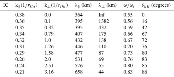
Table 4 shows properties of these waves when damping be-comes 20% of the real frequency. It can be seen that ion cyclotron modes with all angles of propagation (θkB=0–86◦)

are efficiently damped. This implies parallel wave lengths of 360–660 km and minimum perpendicular wave lengths of 40 km (the ion thermal gyroradius used here is 22 km (forTi=2 MK,B=85 nT)). Calculation of the Doppler shifted

theoretical spectral breakpoint frequency of the IC waves in Fig. 13d uses the solutions listed in Table 4. WHAMP calculations with B=60 nT (not shown) indicate that the damping of the parallel propagating solution reaches 20% at

kk=0.42 andω=0.46ωi, which is at lower frequency than the

corresponding solution calculated with B=85 nT. Also the obliquely propagating solutions reach the 20 % damping at lower frequencies forB=60 nT.

5.3 Damping of the Ion Bernstein waves

Figure 12 is in the same format as Fig. 8 showing the real (a) and imaginary (b) frequencies, and theE⊥/B⊥−ratio (in

units (mV/m)/nT) (c) of the ion Bernstein (IB) waves as a function ofk⊥. Several curves (with increments of 0.003 and

with cyclic color table) are shown withkk=0.01–0.06. When k⊥<0.7, the real frequency increases to 1.8fI C for all the

solutions. Whenk⊥ increases the real frequency gradually

decreases towardfI C, but then diverges again for solutions

with highestkk.

Maximum damping is obtained for solution withkk=0.06

(orange) (b), but remains still less than 5% of the real frequency below k⊥=10. For the most damped solution

f=1.4fI C,kk=0.06,k⊥=10, andθkB=89.7◦

Damping is negligible for solutions withkk<0.02. For

in-creasedkkthe waves have a magnetic component but become

more electrostatic as kk decreases (c): for kk=0.01, the E⊥/B⊥−ratio is 30 times larger than forkk=0.06. When kk=0, the wave is entirely electrostatic (not shown). Based on

0 0.1 0.2 0.3 0.4 0.5 0.6 0.7 0.8 0.9 1 0

0.5

f/fi

0 0.1 0.2 0.3 0.4 0.5 0.6 0.7 0.8 0.9 1 −1

0 1

γ

/fi

k

||(ωi/vthi)

(a)

(b)

Fig. 11. Solutions from WHAMP code. (a) shows the real part and (b) shows the imaginary part of frequency of the ion cyclotron wave with

k⊥=0 (blue solution continuing to highestkk),k⊥=0.32 (green),k⊥=0.79 (orange),k⊥=1.0 (aqua),k⊥=1.26 (magenta),k⊥=1.58 (yellow), k⊥=2.0 (gray),k⊥=2.51 (blue),k⊥=3.16 (green) normalized to ion cyclotron frequency atB=85 nT as a function ofkk.

Table 4. Properties of Ion Cyclotron waves (IC) when damping becomes 20% of the real frequency (calculated from WHAMP model with

Maxwellian electron and proton species). Columns list parallel and perpendicular wave numbers and wave lengths, real frequency and wave propagation angle with respect to magnetic field. Ion cyclotron radius,rt hi, used here is 22 km.

IC kk(1/rt hi) k⊥(1/rt hi) λk(km) λ⊥(km) ω/ωi θkB(degrees)

0.38 0.0 364 Inf 0.55 0 0.36 0.1 395 1382 0.56 16 0.35 0.32 395 432 0.59 42 0.34 0.79 407 175 0.66 67 0.32 1.0 432 138 0.67 72 0.31 1.26 446 110 0.70 76 0.29 1.58 477 87 0.73 80 0.26 2.0 531 69 0.76 83 0.24 2.51 576 55 0.80 85 0.21 3.16 658 44 0.83 86

as efficient as damping of the KAW or IC waves for the pre-vailing cusp conditions. The IB mode is coupled to the mag-netosonic mode atk⊥<0.5 andf <1.8fI C(not shown here),

but the damping for that mode is negligible belowk⊥<1 and

at the vicinity of thefI C.

5.4 Discussion on Doppler effect and summary

Figure 13 summarizes the results of this section. The first panel shows the observed slopes at the inertial range every minute (using a 8192 pt. window). The second panel shows the ratio of the observed spectral break point frequency (fbf)

to the local ion cyclotron frequency for all four spacecraft between 05:00–06:00 UT (for the same spectra as calculated for panel a). The empty points indicate that the break point was not clearly identifiable. The observed spectral break-point frequency is at the vicinity of the local cyclotron fre-quency between 05:08–05:28 UT, and usually belowfI C

af-ter 05:30 UT. There are few points where the observed break is above thefI C.

As discussed above, only the KAW and IC waves are ef-ficiently damped, so we will calculate the Doppler shift (ac-cording to Eq. 1) for each of these wave modes using the values ofk⊥, kk, ωandθkB listed in Tables 2 and 4. The

Doppler shift is calculated for every minute and the plasma parameters used in these calculations are averaged using a 11.4-s window andθkV=θBV-θkB. We note that the spectral

calculations are using 6.1-min window, so that such a spec-tra has a superposition of the different Doppler-shifted wave modes. However, using 6.1-min averaging of the plasma pa-rameters will underestimate the Doppler-shift for some in-tervals, which is why we use the higher resolution in or-der to get a broaor-der range of Doppler-shifts. In addition to the waves with θkB, the Doppler shift is also calculated

for θkB+180◦, corresponding to the solutions where k has

a component anti-parallel to the magnetic field (i.e. waves propagating tailwards). Panels (c)–(d) show the ratio of the Doppler shifted theoretical spectral breakpoint frequency to

fI C forB=85 nT (corresponding to time at≈05:15 UT) for

0 1 2 3 4 5 6 7 8 9 10 0

1 2

f/fi

0 1 2 3 4 5 6 7 8 9 10

−0.1 0 0.1

γ

/fi

0 1 2 3 4 5 6 7 8 9 10

0 20 40

E/B ((mV/m) /nT)

k₋|(ω

i/vthi)

(a)

(b)

(c)

Fig. 12. Solutions from WHAMP code. (a) shows the real part and (b) shows the imaginary part of frequency of ion Bernstein modes with

kk=0.06 (orange)–kk=0.01 (blue among cluster of lines) normalized to ion cyclotron frequency atB=85 nT as a function ofk⊥. (c) shows E⊥/B⊥-ratios. Note that a cyclic color table is used such thatkk=0.06 (kk= 0.01) is corresponding to the curve with lowest (highest) E⊥/B⊥-ratio and thatkk=0.06-solution is most strongly damped (b).

are assuming that the magnetic field magnitude is at con-stant 85 nT, although the field gradually decreases and has slightly different magnitudes at all spacecraft. The WHAMP curves look quite similar atB=60 nT (corresponding to time at≈05:40 UT) for KAW, and show damping at lower fre-quencies for IC waves.

During times of enhanced flows (associated with D-shaped distributions) the Doppler shift generates a larger envelope in frequency space between parallel and anti-parallel propa-gating solutions (Figs. 13c and d): the waves that are gen-erated below (above) the spacecraft and that are propagat-ing against (along) the flow have decreased (increased) fre-quency from the plasma frame. Sundkvist et al. (2005) show that D-shaped distributions could generate waves along the field lines (propagating in both directions) at the vicinity of the local ion cyclotron frequency. Between 05:08–05:10 UT sc4 is observing the break frequency,fbf, below 0.4fI C in

agreement with the Doppler-shifted solutions of the waves that propagate against the flow (reduced frequency from the plasma frame). During this interval the other three spacecraft observe the break between 0.7–0.9fI C. These correspond

quite nicely to the IC modes that have a smallθkB and

prop-agate along the flow (increased frequency from the plasma frame). Between 05:10–05:12 UT the Doppler-shifted so-lutions do not match the observed break frequencies. The observedfbf are in fact closer to theoretical frequencies in

the plasma frame (see column 6 in Tables 3 and 4). The abso-lute magnitudes for the Doppler-shift during this interval are in range of 0.3–2fI C, so that the waves causing the break

point frequency at 0.7–0.9fI C could be formed by a)

con-vecting spatial structures (zero plasma frequency) along the flow, b) propagating waves that are generated in low field re-gion along the flow, or c) waves that are generated in the high field region and are propagating against the flow. Between 05:12–05:27 UT there is a range of Doppler-shifted waves that match the observedfbf. Between 05:30–05:34 UT the

(a)

(b)

(c)

(d)

Fig. 13. (a) The inertial range slopes calculated every minute using a 8192-point window with FGM data. (b) The ratio of the observed

spectral breakpoint frequencyfbf tofI Cfor the same spectra as calculated for panel (a). The empty points indicate that the break point was

not clearly identifiable. Panels (c)–(d) show the ratio of the Doppler shifted theoretical spectral breakpoint frequency tof_{I C}(atB=85 nT): (c) shows the kinetic Alfv´en wave solutions with values ofk⊥,kk,θkBlisted in Table 2 (d) shows the IC wave solutions according to Table 4.

Note that the Doppler shift for each solution is calculated both forθkB andθkB+ 180◦. The colors correspond to different spacecraft and

the Doppler shift is not calculated for sc2 due to lack of plasma data. The calculation of the Doppler-shift uses 11.4-s averages of variables V andθkV in Eq. (1).

are used, the plasma frame frequency used in Doppler shift calculations would move to lower frequencies andθkBwould

slightly decrease for KAW (see Figs. 9 and 11).

During times when cyclotron harmonics are observed at the stagnant cusp boundary (between 05:25–05:29 UT and 05:45–05:49 UT, see also Figs. 10 and 12 of Nykyri et al., 2004) the Doppler effect is small and these wave trains are more clearly structured and last longer than the waves ob-served during the sheared flows. It thus appears that the wave modes at the stagnant cusp boundary are observed be-cause either a) they are not efficiently damped, or b) bebe-cause the spacecraft are passing through the region where they are constantly being generated, rather than being convected by the flow.

We have here considered the possibility that the broad-band power law spectra may be composed of an inertial range and a dissipation range. The inertial range fluctuations could be generated by lobe reconnection and associated shear flow layers. An energy cascade may take place perpendicular to the magnetic field (approximately along Cluster trajectory).

The break point frequency could be generated by efficient damping of obliquely propagating KAW modes and ion cy-clotron modes.

Another possibility (private communication from D. Sund-kvist) is that instead of single inertial and dissipation ranges, the spectra is formed of two inertial ranges. It may be possi-ble that the first inertial range is caused (as described above) by the cascade of the fluctuations driven by the lobe re-connection time scale. The second inertial range could be caused by the cascade of the fluctuations generated by several sources at the vicinity of the local ion cyclotron frequency.

(b)

(a)

Fig. 14. Power spectra measured by sc4 at 05:41 UT (a) and at 05:47 UT (b) and their spectral slopes at inertial and dissipation range.

Smaller spacecraft separations (of the order ofri) would

be required in order to accurately determine the Doppler ef-fect for the each wave mode at the vicinity of the ion cy-clotron frequency, by using thek-filtering technique. Even better would be to have a cluster of clusters covering differ-ent scales, from MHD to kinetic ion and electron scales.

6 Feeding of the dissipation range

We suggested earlier that the inertial range fluctuations that are in the frequency range of FGM measurements are generated both remotely (perhaps due to lobe reconnection) and locally due to sheared flows arising from reconnection process. In addition, there are sometimes occasions when lo-cal processes generate the harmonic peaks, and these peaks can then feed the dissipation range. Some evidence for this is shown in Fig. 14 which presents power spectral slopes mea-sured by sc4 during 6.1-min intervals centered at 05:41 UT (left) and 05:47 UT (right).

The shape of the spectra during these two intervals is very different: the 05:41 UT-centered interval shows a more con-tinuous spectra with a not-so-clearly observable break point, whereas the 05:47 UT-centered interval shows a clearer break at 0.14 Hz with harmonics in the dissipation range.

Slopes in the inertial range are –1.72 and –1.62 (calculated from the FGM between 0.3 Hz (a) and between 0.015-0.14 Hz (b)), respectively. The break frequency is determined visually and its location can be confirmed by the steepened slope (measured by FGM) of –2.57 between 0.3–0.5 Hz (a) and –2.7 between 0.15-0.5 Hz (b). The purple arrow marks the local ion cyclotron frequency, so for both intervals the break is observed below the proton cyclotron frequency. The dissipation range slope at 05:41 UT is –2.91 and is calcu-lated from STAFF between 0.5–10.0 Hz. In the 05:47 UT-centered interval there is also a steeper slope of –3.34

mea-sured from STAFF between 3.5–10 Hz (which is above the spectral peaks).

The interval centered at 05:41 UT includes an interval of parallel flow of≈100 km/s, presumably associated with lobe reconnection. The total integrated power in the inertial range calculated from FGM between 0.015–0.3 Hz is 0.39 nT2, and the dissipation range power calculated from STAFF between 0.6–10 Hz is 0.0035nT2.

The interval centered at 05:47 UT is during a time when coherent wave trains (similar to 05:26–05:29 UT) with har-monics of the ion cyclotron frequency were observed (see also Figs. 12 and 13 in Nykyri et al. (2004)). The total in-tegrated power between 0.015–0.14 Hz (from FGM) at this time is 0.098 nT2, which is a factor four smaller than during the 05:41 UT-centered interval. However, the fundamental harmonic peak (slightly abovefI C), and its first harmonic,

have piled up power in the dissipation range. The integrated power measured by STAFF between 0.6–10 Hz is 0.0047 nT2 which is about 1.3 times larger than during the 05:41 UT-centered interval. This seems to indicate that some of the power from the inertial range has shifted into the dissipation range. However, we note here that this is not just a temporal effect but spatio-temporal because the spacecraft have moved ∼2300 km between 05:37 UT and 05:50 UT (from the begin-ning of the measurements used in 05:41 UT-centered interval to end of measurements used in 05:47 UT-centered interval).

7 Discussion and conclusions

breakpoint was clear and occurred at the vicinity of the lo-cal ion cyclotron frequency (fI C). We also found examples

of single sloped spectras where break was not as clearly iden-tifiable (see Fig. 14a). During some intervals clear peaks at cyclotron harmonics were superimposed on this broad band spectra

Slopes of the power spectra both in the inertial and dis-sipation ranges vary throughout the cusp crossing, and even in the same intervals can differ by 100% at different space-craft. Although the plasma properties vary on scales of the spacecraft separation (∼600 km), we found no clear corre-lation between any local plasma parameters and the power spectra slopes. However, we did find a correlation between the integrated power of the magnetic field fluctuations and plasma number flux (this is also observed in recent studies by Sundkvist et al., 2005; Grison et al., 2005), indicative that the solar wind interaction with the cusp magnetic field due to lobe reconnection provides free energy for these fluctuations to grow. We also calculated the ratio between the perpen-dicular and parallel power indicating that in both ranges the fluctuations are mostly transverse.

It may be possible that the cusp geometry with reason-ably strong magnetic field (100–60 nT) allows the coexis-tence of both turbulence and discrete wave modes. Indeed, this is shown to be possible in simulations corresponding to the open coronal magnetic field lines (Dmitruk et al., 2004). We have considered two mechanisms for the generation of the spectral breakpoint and double sloped spectra:

1. In terms of inertial and dissipation range: The onset of the inertial range fluctuations (<fI C) could be formed

partly by the Alfv´enic fluctuations that are generated in the lobe reconnection process (propagating Earth-wards) and partly by the velocity shears that arise from the reconnection process. Indeed, we have observed velocity shears of∼100 km/s at the spacecraft separa-tion scale of 600 km. The broadband (power law) na-ture of the spectra may be formed due to the turbulent cascade (operating perpendicularly to the ambient mag-netic field) of these fluctuations. The onset of the dis-sipation range may be caused by damping of the fluc-tuations that cannot be re-supplied by the cascade from the inertial range. We have used the WHAMP code to study the linear damping properties of the waves at the vicinity of the local ion cyclotron frequency. The re-sults show that an efficient damping (20% of the real frequency) is occuring for obliquely propagating kinetic Alfv´en modes withθkB=70–90◦, and for ion cyclotron

modes with all angles of propagation. Damping of the magnetosonic modes and ion Bernstein modes is negli-gible.

2. In terms of two inertial ranges: The first inertial range is generated as described above (one source being at the

ond inertial range may be formed by cascading of the fluctuations that are generated by one or several sources at the vicinity of the local cyclotron frequency. The ob-servations of the single slope spectra at 05:41 UT could indicate that these sources were absent at the vicinity of thefI C, and the spectra is formed by a single inertial

range during this interval. Alternatively, (supporting the first mechanism) it may be possible that during this in-terval the energy cascading time scale is shorter than the damping time scale of the waves.

We will study this possibility of the second inertial range in future by studying unstable distribution functions. Because cusp is not homogeneous, dispersion solvers including gra-dients in the plasma flow would also be necessary.

In order to understand the formation of the first inertial range we plan to do comparisons between the observed iner-tial range slopes with high-resolution 3-D MHD cusp simula-tions. Cuts can be taken through the simulation box in agree-ment with the real Cluster trajectory. Initial results (Adam-son et al., 2005) of this compari(Adam-son look highly promising, suggesting that lobe reconnection process and resulting ve-locity shears play role in generating inertial range fluctua-tions in the high-altitude cusp.

Another interesting topic is the generation of the ion cy-clotron harmonics. They occur at the stagnant cusp bound-ary (05:25–05:29 UT and 05:45–05:49 UT), are electromag-netic in nature and have quite symmetric distribution func-tions. Ion Bernstein waves are mostly electrostatic and are generated by the shell distributions, excluding them as a pos-sible source for the observed harmonics. One possibility is that ion harmonics are generated by the strong velocity shear but have propagated and observed by Cluster at the stagnant cusp boundary. Figures 9 and 10 of Nykyri et al. (2004) show that harmonics appear after 05:25 UT, about 2 min later than the observed large (∼100 km/s) velocity shear at 05:23 UT. It is well known that field-aligned velocity shears can ex-cite waves at many harmonics of thei (Gavrishchaka et al.,

2000; Ganguli et al., 2002). However, if this is the case it is surprising why harmonics are not observed when the lo-cal velocity shear is the strongest. There are smaller slo-cale ≈5–40 km/s gradients in velocity during the harmonics ob-servations (i.e. at 05:47:30 UT), so perhaps the velocity shear mechanism is able to generate harmonics only in narrow range favoring lower magnitudes for shear.

Acknowledgements. Cluster work in the UK and France is

sup-ported by PPARC and CNES respectively. P. J. Cargill also thanks PPARC for the award of a Senior Research Fellowship. We thank J. R. Johnson at Princeton University for helpful discussions on KAW. We also acknowledge D. Sundkvist for suggesting that the double slope spectra could be generated by two inertial ranges. We thank S. Schwartz for confirming the electron temperatures from the PEACE data.

References

Adamson, E. T., Otto, A., and Nykyri, K.: Plasma dynamics in the vicinity of a cusp-like magnetic configuration, SM52A-08 AGU-fall meeting, 2005.

Balogh, A., Dunlop, M. W., Cowley, S. W. H., Southwood, D. J., Thomlinson, J. G., and magnetometer team: The Cluster Mag-netic Field Investigation, Space Sci. Rev., 79, 65–91, 1997. Balogh, A., Carr, C. M., Acu˜na, M. H., Dunlop, M. W., Beek, T. J.,

Brown, P., Fornangon, K.-H., Georgescu, E., Glassmeier, K.-H., Harris, J., Musmann, G., Oddy, T., and Schwingenschuh, K.: The Cluster magnetic field investigation: overview of in-flight perfo-mance and initial results, Ann. Geophys., 19, 1207–1217, 2001. Cargill, P. J., Dunlop, M. W., Lavraud, B., Elphic, R. C., Holland,

D. L., Nykyri, K., et. al.: CLUSTER encounters with the high altitude cusp: Boundary Structure and magnetic field depletions, Ann. Geophys., 22, 1739–1754, 2004.

Cargill, P. J., Lavraud, B., Owen, C. J., Grison, B., Dunlop, M. W., Cornilleau-Wehrlin, N., Escoubet, C. P., Paschmann, G., Phan, T. D., L.Rezeau, Bogdanova, Y., and Nykyri, K.: The Cusp, Outer Magnetospheric Boundaries:Cluster Results, ISSI, Bern, 2005.

Chen, J. S. and Fritz, T. A.: Correlation of cusp MeV helium with turbulent ULF power spectra and its implications, Geophys. Res. Lett., 25, 4113–4116, 1998.

Cornilleau-Wehrlin, N., Chauveau, P., Louis, S., Meyer, A., Nappa, J. M., Perraut, S., Rezeau, L., Robert, P., Roux, A., Villedary, C. D., Conchy, Y. D., Friel, L., Harve, C. C., Hubert, D., la-combe, C., Manning, R., Wouters, F., Lefeuvre, F., Parrot, M., Pincon, J. L., Poirier, B., Kofman, W., and Louarn, P.: The Clus-ter Spatio-Temporal analysis of field fluctuations STAFF Exper-iment, Space Sci. Rev., 79, 107–136, 1997.

Cornilleau-Wehrlin, N., Chanteur, G., Perraut, S., Rezeau, L., Robert, P., Roux, A., de Villedary, C., Canu, P., Maksimovic, M., de Conchy, Y., Lacombe, D. H. C., Lefeuvre, F., Parrot, M., Pinc¸on, J. L., D´ecr´eau, P. M. E., Harvey, C. C., Louarn, P., San-tolik, O., Alleyne, H. S. C., Roth, M., Chust, T., Le Contel, O., and Staff Team: First results obtained by the Cluster STAFF ex-periment, Ann. Geophys., 21, 437–456, 2003.

Cowley, S.: The causes of convection in the Earth’s magnetosphere, A review of developments during the IMF, Rev. Geophys, 20, 531–565, 1982.

Dmitruk, P., Matthaeus, W. H., and Lanzerotti, L. J.: Discrete modes and turbulence in a wave-driven strongly magnetized plasma, Geophys. Res. Lett., 31, doi:10.1029/2004GL021119, 2004.

Dunlop, M. W., Cargill, P. J., Stubbs, T. J., and Woolliams, P.: The high altitude cusps: HEOS 2, J. Geophys. Res., 105, 27 509– 27 517, 2000.

Fuselier, S. A., Trattner, K. J., and Petrinec, S. M.: Cusp observa-tions of high- and low-latitude reconnection for northward inter-planetary magnetic field, J. Geophys. Res., 105, 253–266, 2000. Ganguli, G., Slinker, S., Gavrishchaka, V., and Scales, W.: Low frequency oscillations in a plasma with spatially variable field-aligned flow, Phys. Plasmas, 9, 2321–2329, 2002.

Gavrishchaka, V., Ganguli, G., Scales, W., Slinker, S., Chaston, C., McFadden, J., Ergun, R., and Carlson, C.: Multiscale coherent structures and broadband waves due to parallel inhomogeneous flows, Phys. Rev. Lett., 85, 4285–4288, 2000.

Goldstein, M. L., Roberts, D. A., and Fitch, C. A.: Properties of the fluctuating magnetic helicity in the inertial and dissipa-tion ranges of the solar wind turbulence, J. Geophys. Res., 99, 11 519–11 538, 1994.

Grison, B., Sahraoui, F., Lavraud, B., Chust, T., Cornilleau-Wehrlin, N., R´eme, H., Balogh, A., and Andre, M.: Wave particle interactions in the high-altitude polar cusp: A Cluster case study, Ann. Geophys., 23, 3699–3713, 2005.

Hasegawa, A. and Chen, L.: Kinetic processes in plasma heating by resonant mode conversion of Alfv´en wave, Phys. Fluids, 19 (12), 1924–1934, 1976.

Janhunen, P., Olsson, A., Vaivads, A., and Peterson, W. K.: Gener-ation of Bernstein waves by ion shell distributions in the auroral region, Ann. Geophys., 21, 881–891, 2003.

Kessel, R. L.,Chen, S.-H., Green, J. L., Fung, S. F., Boardsen, S. A., Tan, L., Eastman, T. E., Craven, J. D., and Frank, L. A.: Evidence of high-latitude reconnection during northward IMF: Ha wkeye observations, Geophys. Res. Lett., 23, 583–586, 1996.

Kindel, J. M. and Kennel, C. F.: Topside current instabilities, J. Geophys. Res., 76, 3055–3078, 1971.

Kolmogoroff, A. N.: The local structure of turbulence in incom-pressible viscous fluid for very large Reynolds number, Dokl. Akad. Nauk SSSR, 30, 301–305, 1941.

Kraichnan, R. H.: Inertial-range spectrum of hydromagnetic turbu-lence, Phys. Fluids, 8, 1385–1387, 1965.

Lavraud, B. and Cargill, P. J.: The magnetospheric cusps re-vealed: Results from the CLUSTER mission, Astronomy and Geophysics, 46, 1.32–1.35, 2005.

Lavraud, B., Dunlop, M. W., Phan, T. D., et. al.: Cluster ob-servations of the exterior cusp and its surrounding bound-aries under northward IMF, Geophys. Res. Lett., 29 (20), doi:10.1029/2002GL015464, 2002.

Lavraud, B., Phan, T. D., Dunlop, M. W., Taylor, M. G. G. T., Cargill, P. J., M.Bosqued, J., Dandouras, I., R´eme, H., Sauvaud, J. A., Balogh, A., and Fazakerley, A.: The exterior cusp and its boundary with the magnetosheath under northward IMF: Cluster multi-event analysis, Ann. Geophys., 22, 3039–30554, 2004. Lavraud, B., Fedorov, A., Budnik, E., Thomsen, M. F., Grikoriev,

A., Cargill, P. J., Dunlop, M. W., R´eme, H., Dandouras, I., and Balogh, A.: High-altitude cusp flow dependence on IMF orien-tation: A 3-year Cluster statistical study, J. Geophys. Res., 110, A02209, doi:10.1029/2004JA010804, 2005.

Le, G., Blanco-Cano, X., Russell, C. T., Zhou, X.-W., Mozer, F., Trattner, K. J., Fuselier, S. A., and Anderson, B. J.: Electromag-netic ion cyclotron waves in the high-altitude cusp: Polar obser-vations, J. Geophys. Res., 106, 19 067–19 079, 2001.

Leamon, R. J., Smith, C. W., Ness, N. F., and Matthaeus, W. H.: Observational constraints on the dynamics of the interplanetary magnetic field dissipation range, J. Geophys. Res., 103, 4775– 4787, 1998.

Lysak, R. L. and Lotko, W.: On the kinetic dispersion relation for shear Alfv´en waves, J. Geophys. Res., 101, 5085–5094, 1996. Nykyri, K., Cargill, P. J., Lucek, E., Horbury, T. S., Balogh, A.,

Lavraud, B., Dandouras, I., and R`eme, H.: Ion cyclotron waves in the high altitude cusp: CLUSTER observations at varying spacecraft separations, Geophys. Res. Lett., 30(24), 2263–2269, doi:10.1029/2003GL018594, 2003.

field fluctuations in the high-altitude cusp, Ann. Geophys., 22, 2413–2429, 2004.

Paschmann, G., Haerendel, G., Sckopke, N., Rosenbauer, H., and Hedgecock, P. C.: Magnetic field characteristics of the distant polar cusp near local noon: the entry layer, J. Geophys. Res., 81, 2883–2899, 1976.

Penano, J. R. and Ganguli, G.: Generation of electromag-netic ion cyclotron waves in the ionosphere by localized transverse dc electric fields, J. Geophys. Res., 107 (A8), doi:10.1029/2001JA000279, 2002.

R`eme, H., Aoustin, C., Bosqued, J. M., Dandouras, I., Lavraud, B., et. al.: First multispacecraft ion measurements in and near the Earth’s magnetosphere with the identical Cluster ion spectrome-try (CIS) experiment, Ann. Geophys., 19, 1303–1354, 2001. Reynolds, M. A. and Ganguli, G.: Ion Bernstein waves driven by

two transverse flow layers, Phys. Plasmas, 5, 2504–2512, 1998. R¨onnmark, K.: Waves in homogenous, anisotropic multicomponent

plasmas (WHAMP), KRI, Tech. rep., 1982.

Russell, C. T., Le, G., and Petrinec, S. M.: Cusp observations of high-and low-latitude reconnection for northward IMF: An alter-nate view, J. Geophys. Res., 105, 5489–5495, 2000.

Sahraoui, F., Pincon, J., Belmont, G., Rezeau, L., Cornilleau-Wehrlin, N., Robert, P., Mellul, L., Bosqued, J., Balogh, A., Canu, P., and Chanteur, G.: ULF wave identification in the mag-netosheath: The k-filtering technique applied to Cluster II data, J. Geophys. Res., 108, 1–1, 2003.

Savin, S. P., Romanov, S. A., Fedorov, A. O., Zelenyi, L., Klimov, S. I., Yermolaev, Y. I., Budnik, E. Y., Nikolaeva, N. S., Rus-sell, C. T., Zhou, X. W., Urguhart, A. L., and Reiff, P. H.: The cusp/magnetosheath interface on May 29, 1996: Interball-1 a nd Polar observations, Geophys. Res. Lett., 3015–3018, 1998. Savin, S. P., Zelenyi, L., Maynard, N. C., Sandahl, I., Kawano,

H., Russell, C. T., Romanov, S., Blecki, J., and et al.: Multi-Spacecraft Tracing of Turbulent Boundary Layer, Adv. Space Res., 30(12), 2821–2830, 2002.

Amata, E., Avanov, L., Blecki, J., et al.: Magnetosheath-cusp interface, Ann. Geophys., 22, 183–212, 2004.

Scudder, J. D., Mozer, F. S., Maynard, N. C., and Russell, C. T.: Fingerprints of collisionless reconnection at the separator, J. Geophys. Res., 107, SMP13–1 to SMP13–38, 2002.

Stasiewicz, K., Bellan, P., Chaston, C., Kletzing, C., Lysak, R., Maggs, J., Pokhotelov, O., Seyler, C., Shukla, P., Stenflo, L., Streltsov, A., and Wahlund, J.-E.: Small Scale Alfv´enic Struc-ture in the Aurora, Space Sci. Rev., 92, 423–533, 2000. Sundkvist, D., Vaivads, A., Andr´e, M., Wahlund, J.-E., Hobara, Y.,

Joko, S., Krasnoselskikh, V. V., Bogdanova, Y. V., Buchert, S. C., Cornilleau-Wehrlin, N., Fazakerley, A., Hall, J.-O., R`eme, H., and Stenberg, G.: Multi-spacecraft determination of wave char-acteristics near the proton gyrofrequency in high-altitude cusp, Ann. Geophys., 23, 983–995, 2005.

Twitty, C., Phan, T. D., Paschmann, G., Lavraud, B., R`eme, H., and Dunlop, M.: Cluster survey of cusp reconnection and its IMF dependence, Geophys. Res. Lett., 31, L19808, doi:10.1029/2004GL020646, 2004.

Vontrat-Reberac, A., Bosqued, J. M., Taylor, M. G., Lavraud, B., Fontaine, D., Dunlop, M. W., Laakso, H., Cornilleau-Werhlin, N., Canu, P., and Fazarkerley, A.: Cluster obser-vations of the high-altitude cusp for northward interplanetary magnetic field: a case study, J. Geophys. Res., 108(A9), doi:10.1029/2002JA001717, 2003.

Zhou, X. W., Russell, C. T., Le, G., Fuselier, S. A., and Scudder, J. D.: The Polar cusp location and its dependence on dipole tilt, Geophys. Res. Lett., 26, 429–432, 1999.