Faster Gradient-Free Proximal Stochastic Methods for Nonconvex Nonsmooth Optimization

(1)

The Thirty-Third AAAI Conference on Artificial Intelligence (AAAI-19)

Faster Gradient-Free Proximal Stochastic

Methods for Nonconvex Nonsmooth Optimization

Feihu Huang,

1,2

_{Bin Gu,}

3

_{Zhouyuan Huo,}

2

_{Songcan Chen,}

1∗

_{Heng Huang}

2,3

1_{College of Computer Science & Technology, Nanjing University of Aeronautics and Astronautics, Nanjing, 211106, China}

2_{Department of Electrical & Computer Engineering, University of Pittsburgh, PA 15261, USA} 3_{JDDGlobal.com}

[email protected], [email protected], [email protected], [email protected], [email protected]

Abstract

Proximal gradient method has been playing an important role to solve many machine learning tasks, especially for the non-smooth problems. However, in some machine learning prob-lems such as the bandit model and the black-box learning problem, proximal gradient method could fail because the ex-plicit gradients of these problems are difficult or infeasible to obtain. The gradient-free (zeroth-order) method can address these problems because only the objective function values are required in the optimization. Recently, the first zeroth-order proximal stochastic algorithm was proposed to solve the non-convex nonsmooth problems. However, its convergence rate isO(_√1

T)for the nonconvex problems, which is significantly slower than the best convergence rateO(1

T)of the zeroth-order stochastic algorithm, whereT is the iteration number. To fill this gap, in the paper, we propose a class of faster zeroth-order proximal stochastic methods with the variance reduction techniques of SVRG and SAGA, which are denoted as ZO-ProxSVRG and ZO-ProxSAGA, respectively. In theo-retical analysis, we address the main challenge that an unbi-ased estimate of the true gradient does not hold in the zeroth-order case, which was required in previous theoretical analy-sis of both SVRG and SAGA. Moreover, we prove that both ZO-ProxSVRG and ZO-ProxSAGA algorithms haveO(_T1)

convergence rates. Finally, the experimental results verify that our algorithms have a faster convergence rate than the existing zeroth-order proximal stochastic algorithm.

Introduction

Proximal gradient (PG) methods (Mine and Fukushima, 1981; Nesterov, 2004; Parikh, Boyd, and others, 2014) are a class of powerful optimization tools in artificial intelligence and machine learning. In general, it considers the following nonsmooth optimization problem:

min

x∈Rd

f(x) +ψ(x), (1)

wheref(x)usually is the loss function such as hinge loss and logistic loss, andψ(x)is the nonsmooth structure regu-larizer such as `1-norm regularization. In recent research,

Beck and Teboulle (2009); Nesterov (2013) proposed the accelerate PG methods to solve convex problems by using

∗

Corresponding Author.

the Nesterov’s accelerated technique. After that, Li and Lin (2015) presented a class of accelerated PG methods for non-convex optimization. More recently, Gu, Huo, and Huang (2018) introduced inexact PG methods for nonconvex nons-mooth optimization. To solve the big data problems, the in-cremental or stochastic PG methods (Bertsekas, 2011; Xiao and Zhang, 2014) were developed for large-scale convex optimization. Correspondingly, Ghadimi, Lan, and Zhang (2016); Reddi et al. (2016) proposed the stochastic PG meth-ods for large-scale nonconvex optimization.

However, in many machine learning problems, the ex-plicit expressions of gradients are difficult or infeasible to obtain. For example, in some complex graphical model in-ference (Wainwright, Jordan, and others, 2008) and struc-ture prediction problems (Sokolov, Hitschler, and Riezler, 2018), it is difficult to compute the explicit gradients of the objective functions. Even worse, in bandit (Shamir, 2017) and black-box learning (Chen et al., 2017) prob-lems, only the objective function values are available (the explicit gradients cannot be calculated). Clearly, the above PG methods will fail in dealing with these scenarios. The gradient-free (zeroth-order) optimization method (Nesterov and Spokoiny, 2017) is a promising choice to address these problems because it only uses the function values in opti-mization process. Thus, the gradient-free optiopti-mization meth-ods have been increasingly embraced for solving many ma-chine learning problems (Conn, Scheinberg, and Vicente, 2009).

Although many gradient-free methods have recently been developed and studied (Agarwal, Dekel, and Xiao, 2010; Nesterov and Spokoiny, 2017; Liu et al., 2018b), they often suffer from the high variances of zeroth-order gradient esti-mates. In addition, these algorithms are mainly designed for smooth or convex settings, which will be discussed in the be-low related works, thus limiting their applicability in a wide range of nonconvex nonsmooth machine learning problems such as involving the nonconvex loss functions and nons-mooth regularization.

In this paper, thus, we propose a class of faster gradient-free proximal stochastic methods for solving the nonconvex nonsmooth problem as follows:

min

x∈Rd

F(x) =:f(x) +ψ(x), f(x) =: 1

n

X

i=1

(2)

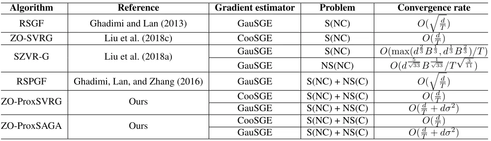
Table 1: Comparison of representative zeroth-order stochastic algorithms for finding an-approximate stationary point of non-convex problem, i.e.,Ek∇f(x)k2 ≤ or Ekgη(x)k2 ≤ . (S, NS, C and NC are the abbreviations of smooth, nonsmooth,

convex and nonconvex, respectively.Tis the whole iteration number,dis the dimension of data andndenotes the sample size.) B(≤n)is a mini-batch size.

Algorithm Reference Gradient estimator Problem Convergence rate

RSGF Ghadimi and Lan (2013) GauSGE S(NC) O(

q

d T)

ZO-SVRG Liu et al. (2018c) CooSGE S(NC) O(_Td)

SZVR-G Liu et al. (2018a) GauSGE S(NC) O(max(d

2 3B

1 3, d

1 3B

2 3)/T)

GauSGE NS(NC) O(d√533B

1 √

33/T

√

3 11)

RSPGF Ghadimi, Lan, and Zhang (2016) GauSGE S(NC) + NS(C) O(

q

d T)

ZO-ProxSVRG Ours CooSGE S(NC) + NS(C) O(

d T)

GauSGE S(NC) + NS(C) O(d

T +dσ

2₎

ZO-ProxSAGA Ours CooSGE S(NC) + NS(C) O(

d T)

GauSGE S(NC) + NS(C) O(_Td +dσ2)

where eachfi(x)is anonconvexand smooth loss function,

andψ(x) is a convex andnonsmoothregularization term. Until now, there are few zeroth-order stochastic methods for solving the problem (2) except a recent attempt pro-posed in (Ghadimi, Lan, and Zhang, 2016). Specifically, Ghadimi, Lan, and Zhang (2016) have proposed a random-ized stochastic projected gradient-free method (RSPGF), i.e., a zeroth-order proximal stochastic gradient method. However, due to the large variance of zeroth-order estimated gradient generated from randomly selecting the sample and the direction of derivative, the RSPGE only has a conver-gence rateO(√1

T), which is significantly slower thanO(

1

T),

the best convergence rate of the zeroth-order stochastic al-gorithm. To accelerate the RSPGF algorithm, we use the variance reduction strategies in the first-order methods,i.e., SVRG (Xiao and Zhang, 2014) and SAGA (Defazio, Bach, and Lacoste-Julien, 2014), to reduce the variance of esti-mated stochastic gradient.

Although SVRG and SAGA have shown good perfor-mances, applying these strategies to the zeroth-order method

is not a trivial task. The main challenge arises due to

that both SVRG and SAGA rely on the assumption that a stochastic gradient is anunbiasedestimate of the true full gradient. However, it does not hold in the zeroth-order al-gorithms. In the paper, thus, we will fill this gap between zeroth-order proximal stochastic method and the classic variance reduction approaches (SVRG and SAGA).

Main Contributions

In summary, our main contributions are summarized as fol-lows:

• We propose a class of faster gradient-free proximal stochastic methods (ZO-ProxSVRG and ZO-ProxSAGA), based on the variance reduction techniques of SVRG and SAGA. Our new algorithms only use the objective func-tion values in the optimizafunc-tion process.

• Moreover, we provide the theoretical analysis on the con-vergence properties of both new ProxSVRG and

ZO-ProxSAGA methods. Table 1 shows the specifical conver-gence rates of the proposed algorithms and other related ones. In particular, our algorithms have faster conver-gence rate O(1

T)thanO(

1

√

T)of the RSPGF (Ghadimi,

Lan, and Zhang, 2016) (the existing stochastic PG algo-rithm for solving nonconvex nonsmoothing problems). • Extensive experimental results and theoretical analysis

demonstrate the effectiveness of our algorithms.

Related Works

Gradient-free (zeroth-order) methods have been effectively used to solve many machine learning problems, where the explicit gradient is difficult or infeasible to obtain, and have also been widely studied. For example, Nesterov and Spokoiny (2017) proposed several random gradient-free methods by using Gaussian smoothing technique. Duchi et al. (2015) proposed a zeroth-order mirror descent al-gorithm. More recently, Yu et al. (2018); Dvurechensky, Gasnikov, and Gorbunov (2018) presented the accelerated zeroth-order methods for the convex optimization. To solve the nonsmooth problems, the zeroth-order online or stochas-tic ADMM methods (Liu et al., 2018b; Gao, Jiang, and Zhang, 2018) have been introduced.

(3)

Although the above zeroth-order stochastic methods can effectively solve the nonconvex optimization, there are few zeroth-order stochastic methods for the nonconvex nons-mooth composite optimization except the RSPGF method presented in (Ghadimi, Lan, and Zhang, 2016). In addition, Liu et al. (2018a) have also studied the zeroth-order algo-rithm for solving the nonconvex nonsmooth problem, which is different from problem (2).

Zeroth-Order Proximal Stochastic Method

Revisit

In this section, we briefly review the zeroth-order proxi-mal stochastic gradient (ZO-ProxSGD) method to solve the problem (2). Before that, we first revisit the proximal gradi-ent descgradi-ent (ProxGD) method (Mine and Fukushima, 1981). ProxGD is an effective method to solve the problem (2) via the following iteration:

xt+1=Proxηψ xt−η∇f(xt)

, t= 0,1,· · · , (3)

whereη > 0 is a step size, and Proxηψ(·) is aproximal

operatordefined as:

Proxηψ(x) = arg min

y∈Rd

ψ(y) + 1

2ηky−xk

2 _.

(4)

As discussed above, because ProxGD needs to compute the gradient at each iteration, it cannot be applied to solve the problems, where the explicit gradient of functionf(x)is not available. For example, in the black-box machine learn-ing model, only function values (e.g., prediction results) are available Chen et al. (2017). To avoid computing explicit gradient, we use the zeroth-order gradient estimators (Nes-terov and Spokoiny, 2017; Liu et al., 2018c) to estimate the gradient only by function values.

• Specifically, we use the Gaussian Smoothing Gradient

Estimator (GauSGE) (Nesterov and Spokoiny, 2017; Ghadimi, Lan, and Zhang, 2016) to estimate the gradients as follows:

ˆ

∇fi(x) =

fi(x+µui)−fi(x)

µ ui, i∈[n], (5) whereµ is a smoothing parameter, and{ui}ni=1 denote

i.i.d.random directions drawn from a zero-mean isotropic multivariate Gaussian distributionN(0, I).

• Moreover, to obtain better estimated gradient, we can use the Coordinate Smoothing Gradient Estimator

(CooSGE) (Gu, Huo, and Huang, 2016; Gu et al., 2018;

Liu et al., 2018c) to estimate the gradients as follows:

ˆ

∇fi(x) = d

X

j=1

fi(x+µjej)−fi(x−µjej)

2µj

ej, i∈[n],

(6)

whereµj is a coordinate-wise smoothing parameter, and

ejis a standard basis vector with1at itsj-th coordinate,

and0otherwise. Although the CooSGE need more func-tion queries than the GauSGE, it can get better estimated gradient, and even can make the algorithms to obtain a faster convergence rate.

Finally, based on these estimated gradients, we give a zeroth-order proximal gradient descent (ZO-ProxGD) method, which performs the following iteration:

xt+1=Proxηψ xt−η∇ˆf(xt)

, t= 0,1,· · · , (7)

where∇ˆf(x) = 1

n

Pn

i=1∇ˆfi(x).

Since ZO-ProxGD needs to estimate full gradient

ˆ

∇f(x) = 1_nPn

i=1∇fi(x), when n is large in the

prob-lem (2), its high cost per iteration is prohibitive. As a result, Ghadimi, Lan, and Zhang (2016) proposed the RSPGF (i.e., ZO-ProxSGD) with performing the following iteration:

xt+1=Proxηψ xt−η∇ˆfIt(xt)

, t= 0,1,· · · , (8)

where ∇ˆfIt(xt) =

1

b

P

i∈It

ˆ

∇fi(x),It ∈ {1,2,· · ·, n}

andb=|It|is the mini-batch size.

New Faster Zeroth-Order Proximal Stochastic

Methods

In this section, to efficiently solve the large-scale nonconvex nonsmooth problems, we propose a class of faster zeroth-order proximal stochastic methods with the variance reduc-tion (VR) techniques of SVRG and SAGA, respectively.

ZO-ProxSVRG

In the subsection, we propose the zeroth-order proximal SVRG (ZO-ProxSVRG) method by using VR technique of SVRG in (Xiao and Zhang, 2014; Reddi et al., 2016).

The corresponding algorithmic framework is described in Algorithm 1, where we use a mixture stochastic gra-dient vˆst = ˆ∇fIt(x

s

t)−∇ˆfIt(˜x

s_{) + ˆ}_∇_f_(˜_xs₎_{. Note that}

EIt[ˆv

s

t] = ˆ∇f(xst) =6 ∇f(xst),i.e., this stochastic

gradi-ent is abiasedestimate of the true full gradient. Although the SVRG has shown a great promise, it relies upon the assumption that the stochastic gradient is an unbiased es-timate of the true full gradient. Thus, adapting the similar ideas of SVRG to zeroth-order optimization is not a trivial task. To address this issue, we analyze the upper bound for the variance of the estimated gradientvˆs

t, and choose the

ap-propriate step sizeη and smoothing parameterµto control this variance, which will be in detail discussed in the below theorems.

Next, we derive the upper bounds for the variance of es-timated gradientvˆs

tbased on the CooSGE and the GauSGE,

respectively.

Lemma 1. In Algorithm 1 using the CooSGE, given the

mixture estimated gradientvˆs

t = ˆ∇fIt(x

s

t)−∇ˆfIt(˜x

s_{) +}

ˆ

∇f(˜xs), then the following inequality holds

Ekvˆts− ∇f(x s t)k

2_≤2δnL2d

b Ekx

s t−˜x

s_k2₊L2d2µ2

2 ,

(9)

where0≤δn≤1.

Remark 1. Lemma 1 shows that variance ofˆvs

t has an

up-per bound. As the number of iterations increases, both xs t

(4)

Lemma 2. In Algorithm 1 using the GauSGE, given the es-timated gradientvˆs

t = ˆ∇fIt(x

s

t)−∇ˆfIt(˜x

s_{) + ˆ}_∇_f_(˜_xs₎_,

then the following inequality holds

Ekvˆst− ∇f(xt)k2≤(2 +

12δn

b )(d+ 6)

3_L2_µ2

+6δnL

2

b Ekx

s t−x˜

s_k2_{+ (4 +}24δn

b )(2d+ 9)σ

2_.

(10)

Remark 2. Lemma 2 shows that variance ofvˆs

t has an

up-per bound. As the number of iterations increases, both xs t

andx˜s_{will approach the same stationary point}_x∗_{, then the}

variance of stochastic gradient decreases.

Algorithm 1ZO-ProxSVRG for Nonconvex Optimization

1: Input:mini-batch sizeb,S,mand step sizeη >0;

2: Initialize:x1

0= ˜x1∈Rd;

3: fors= 1,2,· · ·, Sdo

4: ∇ˆf(˜xs_{) =} 1

n

Pn

i=1∇ˆfi(˜xs);

5: fort= 0,1,· · · , m−1do

6: Uniformly randomly pick a mini-batch It ⊆

{1,2,· · ·, n}such that|It|=b;

7: Using (5) or (6) to estimate mixture stochastic gra-dientˆvs

t = ˆ∇fIt(x

s

t)−∇ˆfIt(˜x

s_{) + ˆ}_∇_f_(˜_xs₎_;

8: xs

t+1=Proxηψ(xts−ηˆvts);

9: end for

10: x˜s+1₌_xs mandx

s+1

0 =xsm;

11: end for

12: Output: Iterate x chosen uniformly random from

{(xst)mt=1}Ss=1.

ZO-ProxSAGA

In the subsection, we propose the zeroth-order proximal SAGA (ZO-ProxSAGA) method via using VR technique of SAGA in (Defazio, Bach, and Lacoste-Julien, 2014; Reddi et al., 2016).

The corresponding algorithmic description is given in Al-gorithm 2, where we use a mixture stochatic gradientvˆt =

1

b

P

it∈It

ˆ

∇fit(xt)− ∇fit(z

t it)

+ ˆφt. Similarly,EIt[ˆvt] =

ˆ

∇f(xst)6=∇f(xst),i.e., this stochastic gradient is abiased

estimate of the true full gradient. Note that in Algorithm 2, due toP

it∈It

ˆ

∇fit(z

t+1

it ) = P

it∈It

ˆ

∇fit(xt), the step 8 can use directly the termP

it∈It

ˆ

∇fit(xt)−∇ˆfit(z

t it)

, which is computed in the step 5, to avoid unnecessary cal-culations. Next, we give the upper bounds for the variance of stochastic gradient ˆvt based on the CooSGE and the

GauSGE, respectively.

Lemma 3. In Algorithm 2 using the CooSGE, given the

esti-mated gradientˆvt= 1_bPit∈It

ˆ

t it)

+ ˆφt

withφˆt = _n1P n

i=1∇ˆfi(zti), then the following inequality

holds

Ekˆvt− ∇f(xt)k2≤

2L2_d

nb

n

X

i=1

Ekxt−zitk

2

2+

L2_d2_µ2

2 .

(11)

Remark 3. Lemma 3 shows that variance ofvˆthas an upper

bound. As the number of iterations increases, both xt and

{zt

i}ni=1 will approach the same stationary point, then the

variance of stochastic gradient decreases.

Lemma 4. In Algorithm 2 using GauSGE, given the

esti-mated gradientˆvt=1_bPit∈It

ˆ

t it)

+ ˆφt

withφˆt = _n1P n

i=1∇ˆfi(zti), then the following inequality

holds

Ekˆvt− ∇f(xt)k2≤(2 +

12

b )(d+ 6)

3_L2_µ2

+6L

2

nb

n

X

i=1

Ekxt−zitk

2_{+ (4 +}24

b )(2d+ 9)σ

2_. ₍₁₂₎

Remark 4. Lemma 4 shows that variance ofvˆthas an upper

bound. As the number of iterations increases, both xt and

{zt

i}ni=1 will approach the same stationary pointx∗, then

the variance of stochastic gradient decreases.

Algorithm 2ZO-ProxSAGA for Nonconvex Optimization

1: Input:mini-batch sizeb,T and step sizeη >0;

2: Initialize:x0∈Rd, andzi0=x0fori∈ {1,2,· · ·, n},

ˆ

φ0= _n1P

n

i=1∇ˆfi(z0i);

3: fort= 0,1,· · ·, T −1do

4: Uniformly randomly pick a mini-batch It ⊆

{1,2,· · · , n}(with replacement) such that|It|=b;

5: Using (5) or (6) to estimate mixture stochastic gradi-entˆvt= 1_bP_i_t_∈I_t ∇ˆfit(xt)−∇ˆfit(z

t it)

+ ˆφt;

6: xt+1=Proxηψ(xt−ηvˆt);

7: zt_i+1

t =xtfori∈ Itandz

t+1

i =z t

i fori /∈ It;

8: φˆt+1= ˆφt−n1

P

it∈It

ˆ

∇fit(z

t it)−

ˆ

∇fit(z

t+1

it )

;

9: end for

10: Output: Iterate x chosen uniformly random from

{xt}Tt=1.

Convergence Analysis

In this section, we conduct the convergence analysis of both ZO-ProxSVRG and ZO-ProxSAGA. First, we give some mild assumptions regarding problem (2) as follows:

Assumption 1. For ∀i ∈ {1,2,· · ·, n}, gradient of the

functionfiis Lipschitz continuous with a Lipschitz constant

L >0, such that

k∇fi(x)− ∇fi(y)k ≤Lkx−yk, ∀x, y∈Rd,

which implies

fi(x)≤fi(y) +∇fi(y)T(x−y) +

L

2kx−yk

2_.

Assumption 2. The gradient is bounded ask∇fi(x)k2 ≤

σ2_{for all}_i_{= 1}_,₂_,_{· · ·}_{, n}_.

(5)

used in (Nesterov and Spokoiny, 2017; Liu et al., 2018b), which is relatively stricter than the bounded variance of gra-dient in (Lian et al., 2016; Liu et al., 2018c,a), due to that we need to analyze more complex problem (2) including a non-smooth part. Next, we introduce the standardgradient mapping(Parikh, Boyd, and others, 2014) used in the con-vergence analysis as follows:

gη(x) =

1

η x−Proxηψ(x−η∇f(x))

. (13)

For the nonconvex problems, ifgη(x) = 0, the pointxis a

critical point (Parikh, Boyd, and others, 2014). Thus, we can use the following definition as the convergence metric.

Definition 1. (Reddi et al., 2016) A solutionxis called

-accurate, ifEkgη(x)k2≤for someη >0.

Convergence Analysis of ZO-ProxSVRG

In the subsection, we show the convergence analysis of the ZO-ProxSVRG with the CooSGE (

ZO-ProxSVRG-CooSGE) and the GauSGE (ZO-ProxSVRG-GauSGE),

respectively.

Theorem 1. Assume the sequence{(xs

t)mt=1}Ss=1generated

from Algorithm 1 using theCooSGE, and define a sequence

{ct}mt=1as follows: fors= 1,2,· · ·, S

ct=

 



δnL2dη

b +ct+1(1 +β), 0≤t≤m−1;

0, t=m

(14)

whereβ > 0. LetT = mS,η = _dLρ (0 < ρ < 1

2)andb

satisfies the following inequality:

8ρ2m2

b +ρ≤1, (15)

then we have

Ekgη(xst)k

2_≤E[F(x10)−F(x∗)]

T γ +

L2_d2_µ2_η

4γ , (16)

whereγ = η₂ −Lη2 _and _x∗ _{is an optimal solution of the}

problem(2). Further letb = [n23],m = [n13],ρ = 1

4 and

µ=O(√1

dT), we have

Ekgη(xst)k

2_≤16dLE[F(x10)−F(x∗)]

T +O(

d

T). (17)

Remark 5. Theorem 1 shows that, givenµ=O(√1

dT),b=

[n23]andm= [n

1

3], the ZO-ProxSVRG-CooSGE hasO(d

T)

convergence rate.

Theorem 2. Assume the sequence{(xs

t)mt=1}Ss=1generated

from Algorithm 1 using the GauSGE, and define a sequence

{ct}mt=1as follows: fors= 1,2,· · ·, S

ct=

 



3δnL2η

b +ct+1(1 +β), 0≤t≤m−1;

0, t=m

(18)

whereβ > 0. Letη = _Lρ (0 < ρ < 1₂)and bsatisfies the following inequality:

24ρ2_m2

b +ρ≤1, (19)

then we have

Ekgη(xst)k2≤ E[F(x1

0)−F(x∗)]

T γ + (1 + 6δn

b )(d+ 6)

3L2µ2η

γ + (2 +12δn

b )(2d+ 9) σ2_η

γ ,

(20)

whereγ = η₂ −η2_L_and_x∗_{is an optimal solution of the}

problem(2). Further letb = [n23],m = [n13],ρ = 1

6 and

µ=O( 1

d√T), we have

Ekgη(xst)k

2

≤18LE[F(x

1

0)−F(x∗)]

T +O(

d T)

+O(dσ2). (21)

Remark 6. Theorem 2 shows that givenµ=O( 1

d√T),b=

[n23]andm= [n

1

3], the ZO-ProxSVRG-GauSGE hasO(d

T+

dσ2₎_{convergence rate, in which the part}_O₍_dσ2₎_generates

from the GauSGE.

Convergence Analysis of ZO-ProxSAGA

In this subsection, we provide the convergence analysis of the ZO-ProxSAGA with the CooSGE (

ZO-ProxSAGA-CooSGE) and the GauSGE (ZO-ProxSAGA-GauSGE),

respectively.

Theorem 3. Assume the sequence{xt}Tt=1 generated from

Algorithm 2 using the CooSGE, and define a positive se-quence{ct}Tt=1as follows:

ct=

L2_dη

b +ct+1(1−p)(1 +β) (22)

whereβ > 0. LetcT = 0,η = _Ldρ (0 < ρ < 1₂), and b

satisfies the following inequality:

32ρ2n2

b3 +ρ≤1, (23)

then we have

Ekgη(xt)k2≤ E

[F(x0)−F(x∗)]

T γ +

L2_d2_µ2_η

4γ , (24)

whereγ = η₂ −Lη2 _and_x∗ _{is an optimal solution of the}

problem(2). Further letb= [n23],ρ=1

8 andµ=O(

1

√

dT),

we have

Ekgη(xt)k2≤

64dLE[F(x0)−F(x∗)]

3T +O(

d

T). (25)

Remark 7. Theorem 3 shows that givenµ=O(_√1

dT)and

b = [n23], the ZO-ProxSAGA-CooSGE hasO(d

T)

(6)

Theorem 4. Assume the sequence{xt}Tt=1generated from

Algorithm 2 using the GauSGE, and define a positive se-quence{ct}Tt=1as follows:

ct=

3L2_η

b +ct+1(1−p)(1 +β), (26)

whereβ >0. LetcT = 0,η=_Lρ(0< ρ < 1₂)andbsatisfies

the following inequality:

96ρ2n2

b3 +ρ≤1, (27)

then we have

Ekgη(xt)k2≤E

[F(x0)−F(x∗)]

T γ +

(2 +12_b )(2d+ 9)σ2_η

γ

+(1 +

6

b)(d+ 6)

3_L2_µ2_η

γ , (28)

where γ = ₂1_η −Lη2 _and _x∗ _{is an optimal solution of}

the problem(2). Further let b = [n23],ρ = 1

12 and µ =

O( 1

d√T), we have

Ekgη(xt)k2≤

144LE[F(x0)−F(x∗)]

5T +O(

d

T) +O(dσ

2_).

₍₂₉₎

Remark 8. Theorem 4 shows that givenµ=O( 1

d√T)and

b= [n23], the ZO-ProxSAGA-GauSGE hasO(d

T+dσ

2₎

con-vergence rate, in which the partO(dσ2₎_{generates from the}

GauSGE.

All related proofs are in the supplementary document.

Experiments

In this section, we will compare the proposed algorithms (ProxSVRG-CooSGE, ProxSVRG-GauSGE, ZO-ProxSAGA-CooSGE, ZO-ProxSAGA-GauSGE) with the RSPGF method (Ghadimi, Lan, and Zhang, 2016) on two applications: black-box binary classification and ad-versarial attacks on black-box deep neural networks

(DNNs). Note that the RSPGF uses the GauSGE to estimate

gradient.

Black-Box Binary Classification

Experimental Setup In this experiment, we apply our

al-gorithms to learn the black-box binary classification prob-lem. Specifically, given a set of training samples{ai, li}ni=1,

whereai ∈Rd andli ∈ {−1,1}, we find the optimal

pre-dictorx∈Rdby solving the following problem:

min

x∈Rd

1

n

X

i=1

fi(x) +λ1kxk1+λ2kxk22, (30)

wherefi(x)is the black-box loss function, that only returns

the function value given an input. Here, we specify the non-convexsigmoid lossfunctionfi(x) = _1+exp(1_l

iaTix) in the black-box setting.

Table 2: Real data for black-box binary classification

datasets #samples #f eatures #classes

20news 16,242 100 2

a9a 32,561 123 2

w8a 64,700 300 2

covtype.binary 581,012 54 2

In the experiment, we use the publicly available real datasets1, which are summarized in Table 2. In the algo-rithms, we fix the mini-batch sizeb = 20, the smoothing parametersµ = 1

d√t in the GauSGE and µ =

1

√

dt in the

GooSGE. Meanwhile, we fixλ1=λ2= 10−5, and use the

same initial solutionx0from the standard normal

distribu-tion in each experiment. For each dataset, we use half of the samples as training data, and the rest as testing data.

Experimental Results Figures 1 and 2 show that both

ob-jective values and test losses of the proposed methods faster decrease than the RSPGF method, as the time increases. In particular, both the ZO-ProxSVRG and ZO-ProxSAGA using the CooSGE show the better performances than the counterparts using the GauSGE. From these results, we find that the CooSGE shows the better performances than the CauSGE in estimating gradients. Moreover, these re-sults also demonstrate that both the ZO-ProxSVRG and ZO-ProxSAGA using the CooSGE have a relatively faster convergence rate than the counterparts using the GauSGE. Since the ZO-ProxSAGA has less function query complexity than the ZO-ProxSVRG, it shows the better performances than the ZO-ProxSVRG. For example, the ZO-ProxSVRG-CooSGE needsO(ndS+bdT)function queries, while ZO-SAGA-CooSGE needsO(bdT)function queries.

Adversarial Attacks on Black-Box DNNs

In this experiment, we apply our methods to generate ad-versarial examples to attack a pre-trained neural network model. Following (Chen et al., 2017; Liu et al., 2018c), the parameters of given model are hidden from us and only its outputs are accessible. In this case, we can not compute the gradients by using back-propagation algorithm. Thus, we use the zeroth-order algorithms to find an universal ad-versarial perturbationx ∈ Rd that could fool the samples

{ai ∈ Rd, li ∈ N}ni=1, which can be specified as the

fol-lowing elastic-net attacks to black-box DNNs problem:

min

x∈Rd

1

n

X

i=1

max

Fli(ai+x)−max

j6=li

Fj(ai+x),0

+λ1kxk1+λ2kxk

2

2, (31)

where λ1 and λ2 are nonnegative parameters to balance

attack success rate, distortion and sparsity. Here F(a) = [F1(a),· · ·, FK(a)] ∈ [0,1]K represents the final layer

output of neural network, which is the probabilities of K classes.

1

20news is from the website https://cs.nyu.edu/∼_roweis/data.

(7)

0 50 100 150 200 250 300 10−4

10−3 10−2 10−1 100

CPU time (seconds)

Objective minus best

RSPGF ZO−ProxSAGA−GauSGE ZO−ProxSAGA−CooSGE ZO−ProxSVRG−GauSGE ZO−ProxSVRG−CooSGE

(a) 20news

0 100 200 300 400 500 600 700 800 10−4

10−3 10−2 10−1 100

CPU time (seconds)

(b) a9a

0 500 1000 1500

10−4 10−3 10−2 10−1 100

CPU time (seconds)

Objective minus best RSPGFZO−ProxSAGA−GauSGE ZO−ProxSAGA−CooSGE ZO−ProxSVRG−GauSGE ZO−ProxSVRG−CooSGE

(c) w8a

0 200 400 600 800 1000 1200 1400 1600 10−4

10−3 10−2 10−1 100

CPU time (seconds)

(d) covtype.binary

Figure 1: Objective valueversusCPU time on black-box binary classification.

0 50 100 150 200 250 300 0

0.1 0.2 0.3 0.4 0.5 0.6

CPU time (seconds)

Test error

(a) 20news

0 100 200 300 400 500 600 700 800 0

0.1 0.2 0.3 0.4 0.5 0.6

CPU time (seconds)

Test error

(b) a9a

0 500 1000 1500

0 0.1 0.2 0.3 0.4 0.5 0.6 0.7

CPU time (seconds)

Test error

(c) w8a

0 200 400 600 800 1000 1200 1400 1600 0

0.1 0.2 0.3 0.4 0.5 0.6

CPU time (seconds)

Test error

(d) covtype.binary

Figure 2: Test lossversusCPU time on black-box binary classification.

Following (Liu et al., 2018c), we use a pre-trained DNN2

on the MNIST dataset as the target black-box model, which achieves 99.4%test accuracy. In the experiment, we select n = 10 examples from the same class, and set the batch sizeb= 5and a constant step sizeη = 1/dfor the zeroth-order algorithms, whered = 28×28. In addition, we set λ1= 10−3andλ2= 1in the experiment.

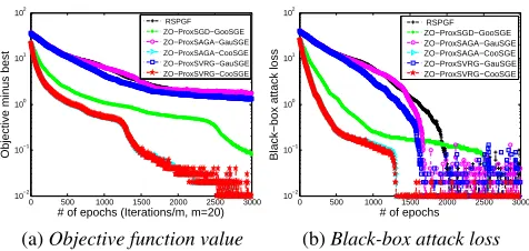
Figure 3 shows that both objective values and black-box attack losses (i.e. the first part of the problem (31)) of the proposed algorithms faster decrease than the RSPGF method, as the number of iteration increases. Here, we add the ZO-ProxSGD-CooSGE method for comparison, which is obtained by combining the ZO-ProxSGD method with the CooSGE. Interestingly, the ZO-ProxSGD-CooSGE shows better performance than both the ZO-ProxSVRG-GauSGE and ZO-ProxSAGA-GauSGE, which further demonstrates that the CooSGE can have better performance than the CauSGE in estimating gradient. Although having a rel-atively good performance in generating the adversarial samples, the ZO-ProxSGD still shows worse performance than both the ZO-ProxSVRG-CooSGE and ZO-ProxSAGA-CooSGE, due to not using the VR technique.

Conclusions

In this paper, we proposed a class of faster gradient-free proximal stochastic methods based on the zeroth-order gra-dient estimators,i.e., the GauSGE and the CooSGE, which only use the objective function values in the

optimiza-2

https://github.com/carlini/nn robust attacks.

0 500 1000 1500 2000 2500 3000 10−2

10−1 100 101 102

# of epochs (Iterations/m, m=20)

RSPGF ZO−ProxSGD−GooSGE ZO−ProxSAGA−GauSGE ZO−ProxSAGA−CooSGE ZO−ProxSVRG−GauSGE ZO−ProxSVRG−CooSGE

(a)Objective function value

0 500 1000 1500 2000 2500 3000 10−2

10−1 100 101 102

# of epochs

Black−box attack loss

RSPGF ZO−ProxSGD−GooSGE ZO−ProxSAGA−GauSGE ZO−ProxSAGA−CooSGE ZO−ProxSVRG−GauSGE ZO−ProxSVRG−CooSGE

(b)Black-box attack loss

Figure 3: Objective value and attack loss on generating ad-versarial samples from black-box DNNs.

tion. Moreover, we provided the theoretical analysis on the convergence properties of the proposed algorithms (ZO-ProxSVRG and ZO-ProxSAGA) based on the CooSGE and the GauSGE, respectively. In particular, both the ZO-ProxSVRG and ZO-ProxSAGA using the CooSGE have rel-atively faster convergence rates than the counterparts using the GauSGE, since the CooSGE has better performance than the CauSGE in estimating gradients.

Acknowledgments

(8)

IIS 1836945, IIS 1836938, DBI 1836866, IIS 1845666, IIS 1852606, IIS 1838627, IIS 1837956.

References

Agarwal, A.; Dekel, O.; and Xiao, L. 2010. Optimal algo-rithms for online convex optimization with multi-point ban-dit feedback. InCOLT, 28–40. Citeseer.

Beck, A., and Teboulle, M. 2009. A fast iterative shrinkage-thresholding algorithm for linear inverse problems. SIAM journal on imaging sciences2(1):183–202.

Bertsekas, D. P. 2011. Incremental proximal methods for large scale convex optimization. Mathematical program-ming129(2):163–195.

Chen, P.-Y.; Zhang, H.; Sharma, Y.; Yi, J.; and Hsieh, C.-J. 2017. Zoo: Zeroth order optimization based black-box attacks to deep neural networks without training substitute models. InThe 10th ACM Workshop on Artificial Intelli-gence and Security, 15–26. ACM.

Conn, A. R.; Scheinberg, K.; and Vicente, L. N. 2009. In-troduction to derivative-free optimization, volume 8. Siam.

Defazio, A.; Bach, F.; and Lacoste-Julien, S. 2014. Saga: A fast incremental gradient method with support for non-strongly convex composite objectives. InAdvances in Neu-ral Information Processing Systems, 1646–1654.

Duchi, J. C.; Jordan, M. I.; Wainwright, M. J.; and Wibisono, A. 2015. Optimal rates for zero-order convex optimization: The power of two function evaluations. IEEE Transactions on Information Theory61(5):2788–2806.

Dvurechensky, P.; Gasnikov, A.; and Gorbunov, E. 2018. An accelerated method for derivative-free smooth stochastic convex optimization. arXiv preprint arXiv:1802.09022.

Gao, X.; Jiang, B.; and Zhang, S. 2018. On the information-adaptive variants of the admm: an iteration complexity per-spective.Journal of Scientific Computing76(1):327–363.

Ghadimi, S., and Lan, G. 2013. Stochastic first- and zeroth-order methods for nonconvex stochastic program-ming. SIAM Journal on Optimization23:2341–2368.

Ghadimi, S.; Lan, G.; and Zhang, H. 2016. Mini-batch stochastic approximation methods for nonconvex stochas-tic composite optimization. Mathematical Programming 155(1-2):267–305.

Gu, B.; Huo, Z.; Deng, C.; and Huang, H. 2018. Faster derivative-free stochastic algorithm for shared memory ma-chines. InICML, 1807–1816.

Gu, B.; Huo, Z.; and Huang, H. 2016. Zeroth-order asyn-chronous doubly stochastic algorithm with variance reduc-tion.arXiv preprint arXiv:1612.01425.

Gu, B.; Huo, Z.; and Huang, H. 2018. Inexact proximal gra-dient methods for non-convex and non-smooth optimization. InAAAI.

Li, H., and Lin, Z. 2015. Accelerated proximal gradient methods for nonconvex programming. InAdvances in neu-ral information processing systems, 379–387.

Lian, X.; Zhang, H.; Hsieh, C. J.; Huang, Y.; and Liu, J. 2016. A comprehensive linear speedup analysis for asyn-chronous stochastic parallel optimization from zeroth-order to first-order. InAdvances in Neural Information Processing Systems, 3054–3062.

Liu, L.; Cheng, M.; Hsieh, C.-J.; and Tao, D. 2018a. Stochastic zeroth-order optimization via variance reduction method.CoRRabs/1805.11811.

Liu, S.; Chen, J.; Chen, P.-Y.; and Hero, A. 2018b. Zeroth-order online alternating direction method of multipliers: Convergence analysis and applications. In The Twenty-First International Conference on Artificial Intelligence and Statistics, volume 84, 288–297.

Liu, S.; Kailkhura, B.; Chen, P.-Y.; Ting, P.; Chang, S.; and Amini, L. 2018c. Zeroth-order stochastic vari-ance reduction for nonconvex optimization. arXiv preprint arXiv:1805.10367.

Mine, H., and Fukushima, M. 1981. A minimization method for the sum of a convex function and a continuously differ-entiable function. Journal of Optimization Theory & Appli-cations33(1):9–23.

Nesterov, Y., and Spokoiny, V. G. 2017. Random gradient-free minimization of convex functions.Foundations of Com-putational Mathematics17:527–566.

Nesterov, Y. 2004. Introductory Lectures on Convex Pro-gramming Volume I: Basic course. Kluwer, Boston.

Nesterov, Y. 2013. Gradient methods for minimizing com-posite functions. Mathematical Programming140(1):125– 161.

Parikh, N.; Boyd, S.; et al. 2014. Proximal algorithms. Foun-dations and TrendsR in Optimization1(3):127–239.

Reddi, S.; Sra, S.; Poczos, B.; and Smola, A. J. 2016. Prox-imal stochastic methods for nonsmooth nonconvex finite-sum optimization. InAdvances in Neural Information Pro-cessing Systems, 1145–1153.

Shamir, O. 2017. An optimal algorithm for bandit and zero-order convex optimization with two-point feedback.Journal of Machine Learning Research18(52):1–11.

Sokolov, A.; Hitschler, J.; and Riezler, S. 2018. Sparse stochastic zeroth-order optimization with an ap-plication to bandit structured prediction. arXiv preprint arXiv:1806.04458.

Wainwright, M. J.; Jordan, M. I.; et al. 2008. Graphical mod-els, exponential families, and variational inference. Founda-tions and TrendsR in Machine Learning1(1–2):1–305.

Xiao, L., and Zhang, T. 2014. A proximal stochastic gradient method with progressive variance reduction. SIAM Journal on Optimization24(4):2057–2075.

Faster Gradient-Free Proximal Stochastic Methods for Nonconvex Nonsmooth Optimization