A relation between algebraic and transform-based reconstruction technique in computed tomography

(1)

Adv. Radio Sci., 11, 95–100, 2013 www.adv-radio-sci.net/11/95/2013/ doi:10.5194/ars-11-95-2013

Advances in

Radio Science

A relation between algebraic and transform-based reconstruction

technique in computed tomography

S. Kiefhaber, M. Rosenbaum, W. Sauer-Greff, and R. Urbansky

Technical University of Kaiserslautern, Chair of Communications Engineering, Germany Correspondence to: S. Kiefhaber ([email protected])

Abstract. In this contribution a coherent relation between the

algebraic and the transform-based reconstruction technique for computed tomography is introduced using the mathemat-ical means of two-dimensional signal processing. There are two advantages arising from that approach. First, the alge-braic reconstruction technique can now be used efficiently regarding memory usage without considerations concerning the handling of large sparse matrices. Second, the relation grants a more intuitive understanding as to the convergence characteristics of the iterative method. Besides the gain in theoretical insight these advantages offer new possibilities for application-specific fine tuning of reconstruction tech-niques.

1 Introduction

Computed tomography is a well-established method in medicine, material science and quality control. It is an imag-ing technique used to create a cross-sectional image of the in-terior of a body to be examined. In contrast to classical imag-ing where the image corresponds directly to the measure-ments, in computed tomography the image is generated in an indirect manner. Therefore a series of transmission mea-surements, e.g. utilising x-rays, is taken. The projection data can be used to reconstruct an image of the inner structure of an object.

Concerning algorithms, the key part of every tomographic imaging system is the reconstruction technique. There are two major reconstruction techniques that are considered in this paper. The first, transform-based approach, was intro-duced in 1917 by the Austrian mathematician Johann Radon (Radon, 1917). The Radon transform and its inverse are ana-lytical expressions of the projection process during the trans-mission measurements and the reconstruction technique, re-spectively. They are well understood from a signal

process-ing point of view. The second, algebraic reconstruction tech-nique is attributed to Bender et al. and, in principal, is an ac-complishment of the Polish mathematician Stefan Kaczmarz who proposed an iterative method to approximate solutions of systems of linear equations (Kaczmarz, 1937). In terms of linear algebra this technique is well known.

The main contribution of this paper is the reinterpretation of the algebraic reconstruction technique by means of two-dimensional signal processing. Starting with the analysis and reinterpretation of the description of the measurement pro-cess using a system of linear equations in Subsect. 3.1 this leads to a mathematical relation between the algebraic and the transform-based reconstruction technique.

Knowledge about this relation has two advantages. First, the algebraic reconstruction technique can now be imple-mented efficiently as to the usage of memory avoiding the necessity to handle large sparse matrices. Second, the closed form of the iteration exactly describes the convergence char-acteristics of the iterative method. In addition to the academ-ical benefit these advantages could offer new possibilities for application-specific fine tuning of reconstruction techniques. The remainder of this publication is organized as follows. A short introduction to the process of data acquisition in computed tomography along with the mathematical descrip-tion of the measured data, namely the Radon transform, is given in Subsect. 2.1. The essential facts about the inverse Radon transform are revisited in Subsect. 2.2 in a intuitive manner based on Morneburg (1995) avoiding the indeed ex-act but also cumbersome mathematical derivation. The prin-cipal ideas of Kaczmarz’ method are summarised in Sub-sect. 2.3. The reinterpretation of the algebraic reconstruction technique is presented in Sect. 3. The proof of the relation between the two methods is given in Subsect. 3.2. The im-plications of the introduced relation between algebraic and transform-based reconstruction technique are discussed in

(2)

96 S. Kiefhaber et al.: A relation between algebraic and transform-based reconstruction technique

2 Kiefhaber et al.: A relation between algebraic and transform-based reconstruction technique in computed tomography

Fig. 1. Measurement of the attenuation of x-rays on their paths along parallels through the phantom repeatedly for different direc-tions, here exemplary for two different angles.

plications of the introduced relation between algebraic and 70

transform-based reconstruction technique are discussed in Subsec. 3.3. A concluding summary of the basic ideas and insights of this contribution is given in Sec. 4.

2 Preliminary Considerations

In this section a short recapitulation of the underlying ideas 75

and the necessary preliminary considerations concerning computed tomography, the transform-based and the algebraic reconstruction technique are given.

2.1 Computed tomography

Computed tomography was first successfully conducted by 80

SIR GODFREY NEWBOLD HOUNSFIELD in 1971 who in 1979 received the Nobel Price in Physiology or Medicine for his efforts together with ALLAN MCLEOD CORMACK. With his device he measured the accumulated attenuation of x-rays on their paths along parallels through the phantom re-85

peatedly for different directions of equally distributed angles between zero and 180 degrees. This is illustrated in Fig. 2.1. Mathematically the measured attenuation can be expressed as the Radon transform of the function describing the spacial distribution of the attenuation coefficient. The local attenua-tion coefficient in a plane(x,y)∈R2 is expressed as a con-tinuous functiong(x,y). The paths are expressed as straight linesG(r,φ) :{(x,y)|0 =r−xcos(φ)−ysin(φ)}whereris the perpendicular distance of G to the origin and φ is the angle betweenGand the y-axis. The ensemble of integrals overg(x,y)along the paths defined byG(r,φ)is the Radon transform

p(r,φ) =R{g(x,y)}=

Z

G(r,φ)

g(x,y)dxdy (1)

and corresponds to the measured data. The main goal in com-puted tomography is to reconstruct the function describing

Fig. 2.Illustration of the backprojection operation.

Fig. 3.Comparison of original and result of plain backprojection

the original spacial distribution of the attenuation coefficient 90

g(x,y)from the integral values measured along parallel paths from different directions as represented by the Radon trans-form p(r,φ). The practical means to solve this problem is given by so-called reconstruction techniques.

For further details on the Radon transform as well as its 95

inverse which is subject to subsection 2.2 please cf. CHOet al. (1993); MORNEBURG (1995); POULARIKAS (1996).

2.2 Transform-based reconstruction technique

Having the Radon transform in mind, the first idea to solve the reconstruction problem is quite manifest, namely inver-sion of the measurement process by backprojecting the inte-gral values onto their respective paths and accumulating the portions from each direction. Mathematically, this backpro-jection can be written as the integral ofp(r,φ)overφ.

B{p(r,φ)}=

π

Z

0

p(r,φ)dφ (2)

The backprojection operation is illustrated in Fig. 2.2. Fig. 2.2 shows the original image as well as the result of the con-100

secutive Radon transform and backprojection. Obviously, the reconstruction resulting from the plain backprojection differs significantly from the original image by a certain blurring ef-fect.

Fig. 1. Measurement of the attenuation of x-rays on their paths

along parallels through the phantom repeatedly for different direc-tions, here exemplary for two different angles.

Subsect. 3.4. A concluding summary of the basic ideas and insights of this contribution is given in Sect. 4.

2 Preliminary Considerations

In this section a short recapitulation of the underlying ideas and the necessary preliminary considerations concerning computed tomography, the transform-based and the algebraic reconstruction technique are given.

2.1 Computed tomography

Computed tomography was first successfully conducted by Sir Godfrey Newbold Hounsfield in 1971 who in 1979 re-ceived the Nobel Price in Physiology or Medicine for his ef-forts together with Allan McLeod Cormack. With his device he measured the accumulated attenuation of x-rays on their paths along parallels through the phantom repeatedly for dif-ferent directions of equally distributed angles between zero and 180 degrees. This is illustrated in Fig. 1.

Mathematically the measured attenuation can be expressed as the Radon transform of the function describing the spacial distribution of the attenuation coefficient. The local attenua-tion coefficient in a plane(x, y)∈_R2is expressed as a con-tinuous functiong(x, y). The paths are expressed as straight linesG(r, φ): {(x, y)|0=r−xcos(φ)−ysin(φ)}whereris the perpendicular distance ofG to the origin and φ is the angle betweenGand the y-axis. The ensemble of integrals overg(x, y)along the paths defined byG(r, φ)is the Radon transform

p(r, φ)=R{g(x, y)} =

Z

G(r,φ)

g(x, y)dxdy (1)

and corresponds to the measured data. The main goal in computed tomography is to reconstruct the function describ-ing the original spacial distribution of the attenuation coeffi-cientg(x, y)from the integral values measured along parallel

Fig. 1. Measurement of the attenuation of x-rays on their paths along parallels through the phantom repeatedly for different direc-tions, here exemplary for two different angles.

plications of the introduced relation between algebraic and 70

transform-based reconstruction technique are discussed in Subsec. 3.3. A concluding summary of the basic ideas and insights of this contribution is given in Sec. 4.

2 Preliminary Considerations

In this section a short recapitulation of the underlying ideas 75

and the necessary preliminary considerations concerning computed tomography, the transform-based and the algebraic reconstruction technique are given.

2.1 Computed tomography

Computed tomography was first successfully conducted by 80

SIR GODFREY NEWBOLD HOUNSFIELD in 1971 who in 1979 received the Nobel Price in Physiology or Medicine for his efforts together with ALLAN MCLEODCORMACK. With his device he measured the accumulated attenuation of x-rays on their paths along parallels through the phantom re-85

peatedly for different directions of equally distributed angles between zero and 180 degrees. This is illustrated in Fig. 2.1. Mathematically the measured attenuation can be expressed as the Radon transform of the function describing the spacial distribution of the attenuation coefficient. The local attenua-tion coefficient in a plane(x,y)∈R2is expressed as a con-tinuous functiong(x,y). The paths are expressed as straight linesG(r,φ) :{(x,y)|0 =r−xcos(φ)−ysin(φ)}whereris the perpendicular distance of G to the origin and φ is the angle betweenGand the y-axis. The ensemble of integrals overg(x,y)along the paths defined byG(r,φ)is the Radon transform

p(r,φ) =R{g(x,y)}=

Z

G(r,φ)

g(x,y)dxdy (1)

and corresponds to the measured data. The main goal in com-puted tomography is to reconstruct the function describing

Fig. 2.Illustration of the backprojection operation.

Fig. 3.Comparison of original and result of plain backprojection

the original spacial distribution of the attenuation coefficient 90

g(x,y)from the integral values measured along parallel paths from different directions as represented by the Radon trans-form p(r,φ). The practical means to solve this problem is given by so-called reconstruction techniques.

For further details on the Radon transform as well as its 95

inverse which is subject to subsection 2.2 please cf. CHOet al. (1993); MORNEBURG (1995); POULARIKAS (1996).

2.2 Transform-based reconstruction technique

Having the Radon transform in mind, the first idea to solve the reconstruction problem is quite manifest, namely inver-sion of the measurement process by backprojecting the inte-gral values onto their respective paths and accumulating the portions from each direction. Mathematically, this backpro-jection can be written as the integral ofp(r,φ)overφ.

B{p(r,φ)}=

π

Z

0

p(r,φ)dφ (2)

The backprojection operation is illustrated in Fig. 2.2. Fig. 2.2 shows the original image as well as the result of the con-100

secutive Radon transform and backprojection. Obviously, the reconstruction resulting from the plain backprojection differs significantly from the original image by a certain blurring ef-fect.

Fig. 2. Illustration of the backprojection operation.

2 Kiefhaber et al.: A relation between algebraic and transform-based reconstruction technique in computed tomography

Fig. 1.

Measurement of the attenuation of x-rays on their paths

along parallels through the phantom repeatedly for different

direc-tions, here exemplary for two different angles.

plications of the introduced relation between algebraic and

70

transform-based reconstruction technique are discussed in

Subsec. 3.3. A concluding summary of the basic ideas and

insights of this contribution is given in Sec. 4.

2 Preliminary Considerations

In this section a short recapitulation of the underlying ideas

75

and the necessary preliminary considerations concerning

computed tomography, the transform-based and the algebraic

reconstruction technique are given.

2.1 Computed tomography

Computed tomography was first successfully conducted by

80

S

IR

G

ODFREY

N

EWBOLD

H

OUNSFIELD

in 1971 who in

1979 received the

Nobel Price in Physiology or Medicine

for his efforts together with A

LLAN

M

C

L

EOD

C

ORMACK

.

With his device he measured the accumulated attenuation of

x-rays on their paths along parallels through the phantom

re-85

peatedly for different directions of equally distributed angles

between zero and 180 degrees. This is illustrated in Fig. 2.1.

Mathematically the measured attenuation can be expressed

as the Radon transform of the function describing the spacial

distribution of the attenuation coefficient. The local

attenua-tion coefficient in a plane

(

x,y

)

∈

_R

2

_{is expressed as a}

con-tinuous function

g

(

x,y

)

. The paths are expressed as straight

lines

G

(

r,φ

) :

{

(

x,y

)

|

0 =

r

−

x

cos(

φ

)

−

y

sin(

φ

)

}

where

r

is

the perpendicular distance of

G

to the origin and

φ

is the

angle between

G

and the y-axis. The ensemble of integrals

over

g

(

x,y

)

along the paths defined by

G

(

r,φ

)

is the Radon

transform

p

(

r,φ

) =

R{

g

(

x,y

)

}

=

Z

G(r,φ)

g

(

x,y

)d

x

d

y

(1)

and corresponds to the measured data. The main goal in

com-puted tomography is to reconstruct the function describing

Fig. 2.

Illustration of the backprojection operation.

Fig. 3.

Comparison of original and result of plain backprojection

the original spacial distribution of the attenuation coefficient

90

g

(

x,y

)

from the integral values measured along parallel paths

from different directions as represented by the Radon

trans-form

p

(

r,φ

)

. The practical means to solve this problem is

given by so-called reconstruction techniques.

For further details on the Radon transform as well as its

95

inverse which is subject to subsection 2.2 please cf. C

HO

et

al. (1993); M

ORNEBURG

(1995); P

OULARIKAS

(1996).

2.2 Transform-based reconstruction technique

Having the Radon transform in mind, the first idea to solve

the reconstruction problem is quite manifest, namely

inver-sion of the measurement process by backprojecting the

inte-gral values onto their respective paths and accumulating the

portions from each direction. Mathematically, this

backpro-jection can be written as the integral of

p

(

r,φ

)

over

φ

.

B{

p

(

r,φ

)

}

=

π

Z

0

p

(

r,φ

)d

φ

(2)

The backprojection operation is illustrated in Fig. 2.2. Fig.

2.2 shows the original image as well as the result of the

con-100

secutive Radon transform and backprojection. Obviously, the

reconstruction resulting from the plain backprojection differs

significantly from the original image by a certain blurring

ef-fect.

Fig. 3. Comparison of original and result of plain backprojection.

paths from different directions as represented by the Radon transformp(r, φ). The practical means to solve this problem is given by so-called reconstruction techniques.

For further details on the Radon transform as well as its inverse which is subject to Subsect. 2.2 please cf. Cho et al. (1993); Morneburg (1995); Poularikas (1996).

2.2 Transform-based reconstruction technique

Having the Radon transform in mind, the first idea to solve the reconstruction problem is quite manifest, namely inver-sion of the measurement process by backprojecting the inte-gral values onto their respective paths and accumulating the portions from each direction. Mathematically, this backpro-jection can be written as the integral ofp(r, φ)overφ.

B{p(r, φ)} =

π Z

0

p(r, φ)dφ (2)

The backprojection operation is illustrated in Fig. 2. Figure 3 shows the original image as well as the result of the consecu-tive Radon transform and backprojection. Obviously, the re-construction resulting from the plain backprojection differs significantly from the original image by a certain blurring ef-fect.

(3)

S. Kiefhaber et al.: A relation between algebraic and transform-based reconstruction technique 97

Kiefhaber et al.: A relation between algebraic and transform-based reconstruction technique in computed tomography 3

Fig. 4. 2D transmission system consisting of Radon transform, backprojection and compensating filter.

The next step towards the solution of the reconstruction 105

problem is to treat the concatenation of Radon transform and backprojection as a two-dimensional linear transmission sys-tem. Thereby it is possible to identify the transmission be-haviour of the system and compensate for it by adding a filter with the inverse behaviour to the signal processing chain. 110

According to DEANS (1983), the impulse response as well as the transfer function of the linear transmission system con-sisting of the concatenation of Radon transform and back-projection decay according to the reciprocal radial distance from the origin, i. e.hRB=1_r andHRB=_f1_r in the original 115

and the Fourier domain, respectively. The functional identity of the impulse responsehRBand the transfer functionHRB is called a fix point of the Hankel transform of order zero which for rotationally symmetric functions is identical to the Fourier transform in two dimensions. The transfer function 120

of the composite systemHRB=_f1

r will play a key role in the derivation of the relation between the transform-based and the algebraic reconstruction technique.

The impulse response of the compensating filter follows from inverting the transfer function HRB and then taking its two-dimensional inverse Fourier transform. Mathemati-cally, the filtering corresponds to a convolution which, incor-porated into Eq. (2), leads to the so-called filtered backpro-jection.

B∗{p(r,φ)}=

π

Z

0

p(r,φ)∗ F₂−1_D{fr}dφ (3)

The filtered backprojection is one representation of the in-verse Radon transform and an analytical solution to the re-125

construction problem. Discretization and implementation leads to the transform-based reconstruction technique. Fig-ure 2.2 illustrates the described construction of the filtered backprojection. The inverse Radon transform can also be de-rived in a strictly mathematical manner as, e. g., shown in 130

POULARIKAS (1996). The strictly mathematical derivation allows to identify the transfer function of the compensating filterfras the determinant of the Jacobian matrix altered due to the transform from Cartesian to polar coordinates which is inherent to the geometry of the measurement process. 135

2.3 Algebraic reconstruction technique

In comparison to transform-based methods, the derivation of the algebraic reconstruction technique follows a somewhat

Fig. 5.Setting up the equation system by defining one linear equa-tion per ray.

different approach. The reconstruction problem is stated di-rectly in a discretised form rather than continuously as for the transform-based reconstruction technique. Figure 2.3 shows a four by four pixel area to be reconstructed which is over-layed with six corridors corresponding to the parallel paths for one exemplary direction. The commonly used approach (see, e. g., KAKet al. (2001)) is to set up one linear equation for each path considering all directions

x1a1,j+x2a2,j+...+xNaN,j=pj (4)

and to combine them to a system of linear equations written here using a vector matrix formalism.

Ax=p (5)

The individual coefficientsai,jmay for example be chosen to account for the intersectional area of the pixeliwith corridor j. Also common practice is to use a hit-or-miss approach in order to reduce the computational effort. If a pixel intersects 140

with the corridor at hand the respective coefficient is set to one, otherwise to zero.

In the linear equation system (5) vector p corresponds to the measured data, matrix A accounts for the geometry of the tomographic system and vectorxcorresponds to the 145

wanted spacial distribution of the attenuation coefficient. On first sight the solution of the reconstruction problem is ob-tained by solving the system of linear equations forx. How-ever, there are certain difficulties that in general prohibit the straight forward solution of Eq. (5).

150

First, matrixAdoes not necessarily need to be square or, second, invertible at all for that matter. Even ifAis a square matrix possible measurement noise might disrupt an exact solution. Third, the mere size of the equation system for any real tomographic system makes a solution, for example using 155

Fig. 4. 2-D transmission system consisting of Radon transform,

backprojection and compensating filter.

The next step towards the solution of the reconstruction problem is to treat the concatenation of Radon transform and backprojection as a two-dimensional linear transmission sys-tem. Thereby it is possible to identify the transmission be-haviour of the system and compensate for it by adding a filter with the inverse behaviour to the signal processing chain.

According to Deans (1983), the impulse response as well as the transfer function of the linear transmission system con-sisting of the concatenation of Radon transform and back-projection decay according to the reciprocal radial distance from the origin, i.e.hRB=1_r andHRB=_f1

r in the original and the Fourier domain, respectively. The functional identity of the impulse responsehRBand the transfer functionHRB

is called a fix point of the Hankel transform of order zero which for rotationally symmetric functions is identical to the Fourier transform in two dimensions. The transfer function of the composite systemHRB=_f1_r will play a key role in

the derivation of the relation between the transform-based and the algebraic reconstruction technique.

The impulse response of the compensating filter follows from inverting the transfer function HRB and then taking

its two-dimensional inverse Fourier transform. Mathemati-cally, the filtering corresponds to a convolution which, incor-porated into Eq. (2), leads to the so-called filtered backpro-jection.

B∗{p(r, φ)} =

π Z

0

p(r, φ)∗F₂−_D1{fr}dφ (3)

The filtered backprojection is one representation of the in-verse Radon transform and an analytical solution to the reconstruction problem. Discretization and implementation leads to the transform-based reconstruction technique. Fig-ure 4 illustrates the described construction of the filtered backprojection. The inverse Radon transform can also be de-rived in a strictly mathematical manner as, e.g., shown in Poularikas (1996). The strictly mathematical derivation al-lows to identify the transfer function of the compensating fil-terfr as the determinant of the Jacobian matrix altered due

to the transform from Cartesian to polar coordinates which is inherent to the geometry of the measurement process.

2.3 Algebraic reconstruction technique

Kiefhaber et al.: A relation between algebraic and transform-based reconstruction technique in computed tomography 3

Fig. 4. 2D transmission system consisting of Radon transform, backprojection and compensating filter.

The next step towards the solution of the reconstruction 105

problem is to treat the concatenation of Radon transform and backprojection as a two-dimensional linear transmission sys-tem. Thereby it is possible to identify the transmission be-haviour of the system and compensate for it by adding a filter with the inverse behaviour to the signal processing chain. 110

According to DEANS (1983), the impulse response as well as the transfer function of the linear transmission system con-sisting of the concatenation of Radon transform and back-projection decay according to the reciprocal radial distance from the origin, i. e. hRB=1_r andHRB=_f1_r in the original 115

and the Fourier domain, respectively. The functional identity of the impulse responsehRBand the transfer functionHRB is called a fix point of the Hankel transform of order zero which for rotationally symmetric functions is identical to the Fourier transform in two dimensions. The transfer function 120

of the composite system HRB=_f1_r will play a key role in the derivation of the relation between the transform-based and the algebraic reconstruction technique.

The impulse response of the compensating filter follows from inverting the transfer function HRB and then taking its two-dimensional inverse Fourier transform. Mathemati-cally, the filtering corresponds to a convolution which, incor-porated into Eq. (2), leads to the so-called filtered backpro-jection.

B∗{p(r,φ)}=

π

Z

0

p(r,φ)∗ F₂−1_D{fr}dφ (3)

The filtered backprojection is one representation of the in-verse Radon transform and an analytical solution to the re-125

construction problem. Discretization and implementation leads to the transform-based reconstruction technique. Fig-ure 2.2 illustrates the described construction of the filtered backprojection. The inverse Radon transform can also be de-rived in a strictly mathematical manner as, e. g., shown in 130

POULARIKAS (1996). The strictly mathematical derivation allows to identify the transfer function of the compensating filterfras the determinant of the Jacobian matrix altered due to the transform from Cartesian to polar coordinates which is inherent to the geometry of the measurement process. 135

2.3 Algebraic reconstruction technique

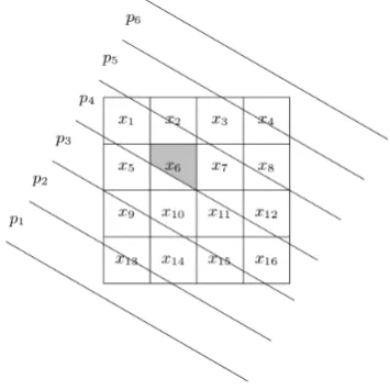
Fig. 5.Setting up the equation system by defining one linear equa-tion per ray.

different approach. The reconstruction problem is stated di-rectly in a discretised form rather than continuously as for the transform-based reconstruction technique. Figure 2.3 shows a four by four pixel area to be reconstructed which is over-layed with six corridors corresponding to the parallel paths for one exemplary direction. The commonly used approach (see, e. g., KAKet al. (2001)) is to set up one linear equation for each path considering all directions

x1a1,j+x2a2,j+...+xNaN,j=pj (4)

Ax=p (5)

The individual coefficientsai,jmay for example be chosen to account for the intersectional area of the pixeliwith corridor j. Also common practice is to use a hit-or-miss approach in order to reduce the computational effort. If a pixel intersects 140

with the corridor at hand the respective coefficient is set to one, otherwise to zero.

In the linear equation system (5) vector p corresponds to the measured data, matrix Aaccounts for the geometry of the tomographic system and vectorx corresponds to the 145

wanted spacial distribution of the attenuation coefficient. On first sight the solution of the reconstruction problem is ob-tained by solving the system of linear equations forx. How-ever, there are certain difficulties that in general prohibit the straight forward solution of Eq. (5).

150

First, matrixAdoes not necessarily need to be square or, second, invertible at all for that matter. Even ifAis a square matrix possible measurement noise might disrupt an exact solution. Third, the mere size of the equation system for any real tomographic system makes a solution, for example using 155

Fig. 5. Setting up the equation system by defining one linear

equa-tion per ray.

different approach. The reconstruction problem is stated di-rectly in a discretised form rather than continuously as for the transform-based reconstruction technique. Figure 5 shows a four by four pixel area to be reconstructed which is over-layed with six corridors corresponding to the parallel paths for one exemplary direction. The commonly used approach (see, e.g., Kak et al., 2001) is to set up one linear equation for each path considering all directions

x1a1,j+x2a2,j+. . .+xNaN,j =pj (4)

Ax=p (5)

The individual coefficientsai,j may for example be chosen to

account for the intersectional area of the pixeliwith corridor

j. Also common practice is to use a hit-or-miss approach in order to reduce the computational effort. If a pixel intersects with the corridor at hand the respective coefficient is set to one, otherwise to zero.

In the linear equation system (5) vector p corresponds to the measured data, matrix A accounts for the geometry of the tomographic system and vector x corresponds to the wanted spacial distribution of the attenuation coefficient. On first sight the solution of the reconstruction problem is ob-tained by solving the system of linear equations for x. How-ever, there are certain difficulties that in general prohibit the straight forward solution of Eq. (5).

First, matrix A does not necessarily need to be square or, second, invertible at all for that matter. Even if A is a square matrix possible measurement noise might disrupt an exact solution. Third, the mere size of the equation system for any real tomographic system makes a solution, for example using

(4)

98 S. Kiefhaber et al.: A relation between algebraic and transform-based reconstruction technique

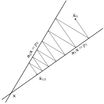
Fig. 6. Move arbitrary pointx0˜ towards the intersectional point of hyperplanes through successive orthogonal projections to find a solution of system of linear equations. Exemplary for first 13 itera-tions

the Moore-Penrose pseudoinverse to approximate a solution, computationally extremely expensive.

Therefore it is advisable to utilize an iterative method to directly determine (in general) an approximationx˜to a solu-tionxof the system of linear equations. In computed tomo-160

graphy there are several methods used such as thealgebraic reconstruction techniqueas suggested by BENDERet al. , the simultaneous iterative reconstruction techniqueor the simul-taneous algebraic reconstruction technique(cf. e. g. KAKet al. (2001)). All of them are in principle based on a method 165

proposed by KACZMARZ (1937).

His idea was to interpretxas a point in ann-dimensional space. Therewith every line of the linear equation system can be used to define a hyperplane in that space. The intersec-tion of all hyperplanes, provided it exists, corresponds to the 170

solution of the system of linear equations. So, to solve the system of linear equations means to find the intersectional point of all hyperplanes. KACZMARZsuggested to do so by choosing an arbitrary point ˜x0 in the n-dimensional space

and moving the initially guessed point towards the real so-175

lution through an iterative process of successive orthogonal projections on the hyperplanes . This process is illustrated for a two-dimensional solution-space in Fig. 2.3.

Mathematically, KACZMARZ’ method can be written as follows. For a detailed derivation cf., e. g., KAK et al. (2001).

˜

xj= ˜xj−1+ a|_j |aj|

(pj−p˜j) where p˜j=aj·x˜j−1 (6)

Here x˜j is the approximation to the solution of the system of linear equations after j orthogonal projections,aj is the j-th line of the coefficient matrixA, andpj is thej-th

mea-sured value andp˜jis the result of the linear mapping defined in (5) assuming˜xj is the wanted spacial distribution of the attenuation coefficient. According to KACZMARZ (1937); TANABE (1971), if for every value ofn one full projection cycle is conducted it follows that in the limitnto infinity˜xn approximates the solution with arbitrary accuracy.

lim

n→∞˜xn=x (7)

Note that if there is no unique solution, the estimate oscillates within the neighbourhood of the intersections.

180

3 Relation of methods

The first step to derive a relation between the inverse Radon transform and KACZMARZ’ method is to reexamine the ini-tial model on which the setup of the system of linear equa-tions is based. This leads to a reinterpretation of KACZ-185

MARZ’ method as iterative backprojection. Thereafter the transmission behaviour of the iterative backprojection will be closely examined by presenting a closed form representation which also exactly describes the convergence characteristics of the iterative method.

190

3.1 Reinterpretation of linear mapping as discretised Radon transform

The representations of the distribution function and the paths in terms of pixels and corridors, respectively, correspond to the usage of a Haar basis; in terms of sampling and interpo-195

lation theory it corresponds to interpolation with B-splines of order zero or, colloquial, to anearest neighbour interpo-lation (cf., e.g., UNSER (2000)). By disregarding the par-ticular method of interpolation the setup of the linear equa-tion system can be done assuming the elements of vectorsx 200

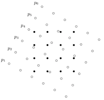
andpbeing the weights of a Dirac basis representations, i. e. the samples of the continuous function describing the spacial distribution of the attenuation coefficients and their directed sums as discretisation of the path integrals, respectively. This is illustrated in Fig. 3.1. The particular method of interpola-205

tion is accounted for by the values of the coefficient matrix A.

From that point of view it becomes comprehensible that depending on the kind of interpolation the system of lin-ear equations (5) is essentially a discretisation of the Radon 210

transform. By applying this idea on Eq. (6) KACZMARZ’ method can be understood as iterative backprojection of the difference between virtual projection datap˜n computed us-ing the estimated distribution function˜xn−1and the actually measured datap.

215

Based on the above considerations Eq. (6) can be rewritten using the Radon transform and backprojection operators on

Fig. 6. Move arbitrary pointx˜0towards the intersectional point of

hyperplanes through successive orthogonal projections to find a so-lution of system of linear equations. Exemplary for first 13 itera-tions.

the Moore-Penrose pseudoinverse to approximate a solution, computationally extremely expensive.

Therefore it is advisable to utilize an iterative method to directly determine (in general) an approximationx to a solu-˜

tion x of the system of linear equations. In computed tomo-graphy there are several methods used such as the algebraic reconstruction technique as suggested by Bender et al., the simultaneous iterative reconstruction technique or the simul-taneous algebraic reconstruction technique (cf. e.g. Kak et al., 2001). All of them are in principle based on a method proposed by (Kaczmarz, 1937).

His idea was to interpret x as a point in ann-dimensional space. Therewith every line of the linear equation system can be used to define a hyperplane in that space. The intersec-tion of all hyperplanes, provided it exists, corresponds to the solution of the system of linear equations. So, to solve the system of linear equations means to find the intersectional point of all hyperplanes. Kaczmarz suggested to do so by choosing an arbitrary point x˜0 in the n-dimensional space

and moving the initially guessed point towards the real so-lution through an iterative process of successive orthogonal projections on the hyperplanes . This process is illustrated for a two-dimensional solution-space in Fig. 6.

Mathematically, Kaczmarz’ method can be written as fol-lows. For a detailed derivation cf., e.g., Kak et al. (2001).

˜

xj= ˜xj−1+

a|_j

|aj|

pj− ˜pj

where p˜j=aj· ˜xj−1 (6) Herex˜j is the approximation to the solution of the system

of linear equations afterj orthogonal projections, aj is the

j-th line of the coefficient matrix A, andpj is thej-th

mea-sured value andp˜jis the result of the linear mapping defined

in (5) assumingx˜j is the wanted spacial distribution of the

attenuation coefficient. According to Kaczmarz (1937); Tan-abe (1971), if for every value ofnone full projection cycle is conducted it follows that in the limitnto infinityx˜n

approx-imates the solution with arbitrary accuracy. lim

n→∞ ˜

xn=x (7)

Note that if there is no unique solution, the estimate oscillates within the neighbourhood of the intersections.

3 Relation of methods

The first step to derive a relation between the inverse Radon transform and Kaczmarz’ method is to reexamine the initial model on which the setup of the system of linear equations is based. This leads to a reinterpretation of Kaczmarz’ method as iterative backprojection. Thereafter the transmission be-haviour of the iterative backprojection will be closely exam-ined by presenting a closed form representation which also exactly describes the convergence characteristics of the iter-ative method.

3.1 Reinterpretation of linear mapping as discretised Radon transform

The representations of the distribution function and the paths in terms of pixels and corridors, respectively, correspond to the usage of a Haar basis; in terms of sampling and interpo-lation theory it corresponds to interpointerpo-lation with B-splines of order zero or, colloquial, to a nearest neighbour interpo-lation (cf., e.g., Unser, 2000). By disregarding the particular method of interpolation the setup of the linear equation sys-tem can be done assuming the elements of vectors x and p be-ing the weights of a Dirac basis representations, i.e. the sam-ples of the continuous function describing the spacial distri-bution of the attenuation coefficients and their directed sums as discretisation of the path integrals, respectively. This is il-lustrated in Fig. 7. The particular method of interpolation is accounted for by the values of the coefficient matrix A.

From that point of view it becomes comprehensible that depending on the kind of interpolation the system of linear Eq. (5) is essentially a discretisation of the Radon transform. By applying this idea on Eq. (6) Kaczmarz’ method can be understood as iterative backprojection of the difference be-tween virtual projection data p˜n computed using the

esti-mated distribution functionx˜n−1and the actually measured datap.

Based on the above considerations Eq. (6) can be rewritten using the Radon transform and backprojection operators on the continuously defined distribution function.

˜

gn+1= ˜gn+B(p−Rg˜n) where p=Rg

= ˜gn+B(Rg−Rg˜n)

= ˜gn+BRg−BRg˜n (8)

(5)

S. Kiefhaber et al.: A relation between algebraic and transform-based reconstruction technique 99

Kiefhaber et al.: A relation between algebraic and transform-based reconstruction technique in computed tomography

5

Fig. 7. Dirac representation of model on which the set up of the system of linear equations is based.

the continuously defined distribution function.

˜

g

n+1

= ˜

g

n

+

B

(

p

− R

g

˜

n

)

where

p

=

R

g

= ˜

g

n

+

B

(

R

g

− R

g

˜

n

)

220

= ˜

g

n

+

BR

g

− BR

˜

g

n

(8)

At this point it is obvious that both reconstruction

tech-niques are not completely independent of each other as, e. g.,

asserted in K

AK

et al.

(2001). Using the means of

two-dimensional signal processing, in particular sampling and

225

interpolation theory K

ACZMARZ

’ method has indeed been

shown to be a kind of iterative backprojection using the

Radon transform to determine the estimation error. In the

following subsection 3.2 the iterative backprojecting will be

shown, for all practical means, to actually have the same

230

transmission behaviour as the inverse Radon transform. This

will also yield an explicit description of the convergence

characteristics of the iterative method.

3.2 Transmission behaviour of iterative backprojection

In order to understand the transmission behaviour of the

it-erative backprojection it is self-evident to take a closer look

at the Fourier space representation of Eq. (8). From

subsec-tion 2.2 it is known that a linear two-dimensional

transmis-sion system consisting of consecutive Radon transform and

(unfiltered) backprojection can be described by an impulse

response as well as a transfer function following

_x1

. Bearing

that in mind the Fourier transform of Eq. (8) can be written

as follows.

˜

G

n+1

= ˜

G

n

+

1 f

r

G

−

1 f

r

˜

G

n

(9)

Here

f

r

is the spacial frequency in radial direction and

G

235

and

G

˜

are the spectra of the actual and estimated distribution

functions, respectively.

The idea for deriving a closed form representation of the

iterative method arises from taking a look at the first four

iteration steps in Fourier space. The initial guess has been

240

chosen according to

G

˜

0

= 0.

˜

G

0

= 0

˜

G

1

=

1 f

r

G

˜

G

2

=

2 f

r

−

1 f

2 r

G

˜

G

3

=

3 f

r

−

3 f

2 r

+

1 f

3 r

G

245

˜

G

4

=

4 f

r

−

6 f

2 r

+

4 f

3 r

−

1 f

4 r

G

The term in brackets can be identified as part of an

alternat-ing binomial series for which the followalternat-ing relationship is

known.

n

X

k=0

n

k

a

n−k

b

k

= (

a

+

b

)

n

(10)

This leads to the assertion that for

f

r

≥

1 and

g

˜

0

= 0

the

fol-lowing relation holds, where

a

= 1

and

b

=

−

1

fr

have been

used in Eq. (10).

˜

G

n

=

1 −

1 f

r

n

G

This can be shown by mathematical induction.

Base case (

n

= 0

)

˜

G

0

=

1 −

1 f

r

0

!

G

= 0

(11)

Inductive step

(

n

→

n

+ 1) using (11) in (9)

˜

G

n+1

=

1 −

1 f

r

n

G

+

1 f

r

G

−

1 f

r

1 −

1 f

r

n

G

=

1 −

1 f

r

n

+

1 f

r

1 −

1 f

r

n

G

250

=

1 −

1 f

r

1 −

1 f

r

n

G

=

1 −

1 f

r

n+1

!

G

Q.E.D.

(12)

(Note that the above identity can also be derived making use

of the fact that Eq. (9) is a linear inhomgenous recursion

formula of first order for which there is a general closed form

255

correspondence.)

Taking the limit of Eq. (12) for

n

to infinity clarifies the

transmission behaviour of the iterative backprojection. By

rewriting the term in brackets it becomes obvious that if

f

r

is

greater than one the bracketed term vanishes in the limit and

Fig. 7. Dirac representation of model on which the set up of the

system of linear equations is based.

At this point it is obvious that both reconstruction tech-niques are not completely independent of each other as, e.g., asserted in Kak et al. (2001). Using the means of two-dimensional signal processing, in particular sampling and in-terpolation theory Kaczmarz’ method has indeed been shown to be a kind of iterative backprojection using the Radon trans-form to determine the estimation error. In the following Sub-sect. 3.2 the iterative backprojecting will be shown, for all practical means, to actually have the same transmission be-haviour as the inverse Radon transform. This will also yield an explicit description of the convergence characteristics of the iterative method.

3.2 Transmission behaviour of iterative backprojection

In order to understand the transmission behaviour of the iter-ative backprojection it is self-evident to take a closer look at the Fourier space representation of Eq. (8). From Sub-sect. 2.2 it is known that a linear two-dimensional transmis-sion system consisting of consecutive Radon transform and (unfiltered) backprojection can be described by an impulse response as well as a transfer function following 1_x. Bearing that in mind the Fourier transform of Eq. (8) can be written as follows.

˜

Gn+1= ˜Gn+

1

fr

G− 1

fr

˜

Gn (9)

Herefr is the spacial frequency in radial direction and G

andG˜ are the spectra of the actual and estimated distribution functions, respectively.

The idea for deriving a closed form representation of the iterative method arises from taking a look at the first four iteration steps in Fourier space. The initial guess has been

chosen according to_G˜

0=0.

˜

G0=0

˜

G1= 1

fr

G

˜

G2=

₂ fr − 1 f2 r G ˜

G3=

₃ fr − 3 f2 r + 1 f3 r G ˜

G4=

₄ fr − 6 f2 r + 4 f3 r − 1 f4 r G

The term in brackets can be identified as part of an alternat-ing binomial series for which the followalternat-ing relationship is known.

n X

k=0

_n

k

an−kbk=(a+b)n (10)

This leads to the assertion that forfr≥1 andg˜0=0 the fol-lowing relation holds, wherea=1 andb= −1

fr have been used in Eq. (10).

˜

Gn=

1−

1− 1

fr n

G

This can be shown by mathematical induction.

3.2.1 Base case (n=0)

˜

G0= 1−

1− 1

fr 0!

G=0 (11)

3.3 Inductive step

(n→n+1) using (11) in (9) ˜

Gn+1=

1−

1− 1 fr

n G+ 1

fr

G− 1 fr

1−

1− 1 fr n G = 1−

1− 1

fr n

+ 1

fr

1− 1

fr n G = 1−

1− 1

fr

1− 1

fr n

G

= 1−

1− 1

fr n+1!

G Q.E.D. (12)

(Note that the above identity can also be derived making use of the fact that Eq. (9) is a linear inhomgenous recursion for-mula of first order for which there is a general closed form correspondence.)

Taking the limit of Eq. (12) fornto infinity clarifies the transmission behaviour of the iterative backprojection. By rewriting the term in brackets it becomes obvious that iffris

greater than one the bracketed term vanishes in the limit and

(6)

100 S. Kiefhaber et al.: A relation between algebraic and transform-based reconstruction technique

the spectrum of the estimated solution_G˜

napproximates the

spectrumGof the actual solution with arbitrary accuracy.

lim

n→∞ ˜

Gn= lim n→∞

1−

_f r−1

fr n

G=G (13) In the original space it then follows for the estimated and actual solutions that

lim

n→∞ ˜

gn=g. (14)

Hence, for frequenciesfr >1 the iterative backprojection

converges to the solution as the term in brackets vanishes in Eq. (13).

3.4 Implications

The first implication regards the stability of the numerical implementation of the algebraic reconstruction technique. For the numerical computation the constrainfr>1 means

that in terms of linear algebra the biggest eigenvalue of the concatenated projection and backprojection has to be lower or equal to one to guarantee convergence. In terms of the Radon and backprojection operators the operator-norm of the concatenation has to be lower or equal to one. Practically, the square sum of the pixel values , i.e. the energy of the recon-struction may not increase from one iteration step to the next. This can, e.g., be ensured by weighting the whole reconstruc-tion with a constant factor. The closer the implementareconstruc-tion is to the stability bound the faster the convergence.

The second implication regards the runtime of the recon-struction techniques. As for every cycle of the iterative back-projection a Radon transform and a backback-projection has to be performed it is obvious that the transform-based reconstruc-tion technique delivers its result in a fracreconstruc-tion of the time that is needed for the algebraic reconstruction technique. Albeit, the exact time needed for the algebraic reconstruction tech-nique depends on the required accuracy of the reconstruction which can be utilized as a criterion to abort the iteration pro-cess.

Last, the introduced relation allows to implement the alge-braic reconstruction technique independently of the vector-matrix formalism avoiding the necessity to deal with han-dling large sparse matrices.

4 Summary

In this contribution the derivation of a relation between the algebraic and the transform-based reconstruction technique in computed tomography was discussed in a very general way. Therefore, based on preliminary considerations, the model for setting up the system of linear equations was rein-terpreted using the means of sampling and interpolation the-ory which lead to understand Kaczmarz’ method as iterative backprojection. The transmission behaviour of the iterative backprojection was examined and characterised offering a closed form representation of the iteration. Finally the impli-cations and advantages of the new relation besides the aca-demical benefit where discussed. The insights offered in this contribution give the means for further application-specific refinement and tuning of reconstruction techniques.

References

Bender, R., Gordon, R., and Herman, G.: Algebraic Reconstruction Techniques (ART) for Three-Dimensional Electron Microscopy and X-Ray Photography, in J. Theoret. Biol., 29, 471–481, 1970. Cho, Z.-H., Jones, J. P., and Singh, M.: Foundations of medical imaging, New York: Wiley, 1993, ISBN 0-471-54573-2, 1993. Deans, S.: The Radon transform and some of its Applications, New

York, Wiley, ISBN 0-471-89804-X, 1983.

Kaczmarz, S.: Angen¨aherte Aufl¨osung von Systemen linearer Gle-ichungen, Bull. Acad. Pol. Sci. Lett., A35, 355–357, 1937. Kak, A., and Slaney, M.: Principles of Computerized Tomographic

Imaging, New York, Society of Industrial and Applied Mathe-matics, ISBN 0-87942-198-3, 2001.

Morneburg, H. (Hrsg.): Bildgebende Systeme für die medizinis-che Diagnostik: Röntgendiagnostik und Angiographie, Comput-ertomographie, Nuklearmedizin, Magnetresonanztomographie, Sonographie, integrierte Informationssysteme. 3., wesentlich überarb. und erw. Aufl. München: Publicis-MCD-Verl., ISBN 3-89578-002-2, 1995.

Poularikas, A., D. (Hrsg.): The transforms and applications hand-book, Boca Raton, Fla.: CRC Press [u.a.], ISBN 0-8493-8342-0, 1996.

Radon, J.: Über die Bestimmung von Funktionen durch ihre Integralwerte längs gewisser Mannigfaltigkeiten, in: Berichte Sächsische Akademie der Wissenschaften, Math.-Phys. Kl., Leipzig, 69, 262–267, 1917.

Tanabe, K.: Projection Method for Solving a Singular System of Linear Equations and its Applications, in: Numer. Math., 17, 1971, 203–214, Springer-Verlag, 1971.

Unser, M.: Sampling–50 Years after Shannon, in: Proceedings of the IEEE, 88, 4, 569–587, Publisher Item Identifier S-0018-9219(00)01299-7, 2000.