Computation of electrostatic ﬁelds in anisotropic human tissues using the Finite Integration Technique (FIT)

(1)

Advances in

Radio Science

Computation of electrostatic fields in anisotropic human tissues

using the Finite Integration Technique (FIT)

V. C. Motrescu and U. van Rienen

Institute of General Electrical Engineering, University of Rostock, Germany

Abstract. The exposure of human body to electromagnetic fields has in the recent years become a matter of great in-terest for scientists working in the area of biology and bio-medicine. Due to the difficulty of performing measurements, accurate models of the human body, in the form of a com-puter data set, are used for computations of the fields in-side the body by employing numerical methods such as the method used for our calculations, namely the Finite Inte-gration Technique (FIT). A fact that has to be taken into account when computing electromagnetic fields in the hu-man body is that some tissue classes, i.e. cardiac and skeletal muscles, have higher electrical conductivity and permittivity along fibers rather than across them. This property leads to diagonal conductivity and permittivity tensors only when ex-pressing them in a local coordinate system while in a global coordinate system they become full tensors. The Finite Inte-gration Technique (FIT) in its classical form can handle di-agonally anisotropic materials quite effectively but it needed an extension for handling fully anisotropic materials. New electric voltages were placed on the grid and a new averag-ing method of conductivity and permittivity on the grid was found. In this paper, we present results from electrostatic computations performed with the extended version of FIT for fully anisotropic materials.

1 Introduction

With continuously increasing numbers of electrical and elec-tronic devices being used both in households and for com-munication purposes, special concerns arise regarding the possible adverse biological effects of high or low frequency electromagnetic fields on the human body. The difficulties in directly measuring the fields’ induced currents or energy inside the body have resulted in different maximum values within the safety guidelines for limiting the effects of human Correspondence to: V. C. Motrescu

([email protected])

exposure to non-ionizing electromagnetic radiation. In such conditions, the estimation of electromagnetic fields inside the body using numerical methods adequate for computer code implementations, represents a good alternative to the experi-mental measurements, especially, because the computational capacities are currently able to respond to such complex tasks and continue to have a quick evolution. Another argument for using computer based numerical methods is the availabil-ity of realistic human body models of high resolution based on anatomical data in the form of a computer data set. Nu-merical methods such as the Finite Element Method (FEM), the Finite Difference Method (FD), the Boundary Element Method (BEM), and the Finite Integration Technique (FIT) have already been used in computations of electromagnetic fields in the human body. Our computations are based on an extended version of the Finite Integration Technique (FIT) which allows us to account for the anisotropic character of some tissue classes.

2 Human body model

(2)

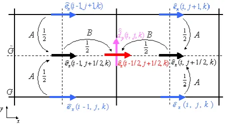
Fig. 1. Local interpolation scheme of a grid voltage in x-direction

at the location of a grid flux in y-direction.

Orientation Data Set which gives the direction of fibers by providing two angles for every voxel containing muscle tis-sue (Sachse et al., 1998).

3 Electromagnetic properties of biological tissues

It is known that biological tissue is non-magnetic i.e. the per-meability of biological tissue is equal to that of free space (Durney et al., 1986). The permittivity and conductivity vary with temperature but a stronger variance is experienced with frequency. While permittivity of biological tissue gen-erally decreases with frequency, its conductivity gengen-erally in-creases.

Some tissue types which present a fiber structure (e.g. skeletal and cardiac muscles) are anisotropic having higher conductivity and permittivity in the longitudinal direction of the fibers than on the perpendicular direction to the fibers (Sachse et al., 1997). Shortly, these tissues present a trans-versely isotropic anisotropy with regard to their dielectric properties.

(Note: In compliance with the subject matter, the remain-der of this paper will refer only to permittivity, though, it should be noted that conductivity can be treated in exactly the same way.)

In a local coordinate system, the permittivity of muscle tissue is described by a diagonal tensor of rank two:

Tεl=

 

εl 0 0

0 εp 0

0 0 εp



, (1)

whereεlis the longitudinal permittivity andεpis the

perpen-dicular permittivity, relative to the fiber’s direction.

Since muscle fibers are miscellaneously oriented in the body, for computational reasons, it is useful to express this tensor in a global coordinate system. In this respect, the local tensor has to be rotated according to the following equation: TεG=RTεLR

−1_, ₍₂₎

where the rotation matrix R is the product of two other rota-tion matrices: R=RxyRxz, with Rxyand Rxzgiven below.

Rxy=

 

cosφ−sinφ0 sinφ cosφ 0

0 0 1



 Rxz=

 

sinθ 0 cosθ

0 1 0

cosθ 0−sinθ  . (3) The anglesφandθare the rotation angles about the z- and y-axes, respectively, provided by the Orientation Data Set. After the rotation in Eq. (2) we obtain a full and symmetric tensor which expresses the permittivity of muscle tissue in a global coordinate system.

4 Considerations concerning the classical Finite Inte-gration Technique (FIT)

Since a lot of literature has already been published about the FIT, only a short introduction is provided here concerning the allocation of some grid-state variables and material treatment related to the subject of this paper. For more general details about FIT, we recommend you see van Rienen (2001), mean-while, for more information concerning the subject matter of this paper, see van Rienen et al. (2003).

The Finite Integration Technique (FIT) was first published by Weiland (1977) and developed as a numerical method which discretizes the Maxwell’s equations on a grid pair preserving the analytical properties of the original equations (van Rienen, 2001). On the FIT’s grid doublet, in connection with Electrostatics, the following variables are defined:

– the electric potentials (denoted withϕn), allocated in

ev-ery mesh node belonging to the primary grid;

– the electric grid voltages (denoted witheˆn), allocated in

the middle of the edges belonging to the primary grid and calculated as the integral of the electric field along primary edges;

– the electric grid flux densities (denoted withdˆˆn), normal

in the middle of the surfaces belonging to the dual grid and calculated as the integral of the electric flux on dual surfaces.

In a 3D Cartesian coordinate system, because the dual grid is shifted with half an edge length in all positive directions with respect to the primary grid, the primary edges intersect dual surfaces on the normal direction in the middle. This means that an electric grid voltageeˆnfrom the primary grid

is allocated in the same point with the corresponding electric grid flux_dˆˆ

nin the same direction, from the dual grid.

The electric fluxes and voltages with coinciding both, lo-cations and orientations, are related to each other by the per-mittivity according to the following equation:

ˆ ˆ dn

ˆ en

= R R

˜

AnD·dA

R

LnE·ds

= R R

˜

AnεdA+O(1

κ+1₎

R

Lnds+O(1

κ₎

≈ε R R

˜

AndA

R

Lnds

+O(1κ)≈ε| ˜An| |Ln|

(3)

whereκ takes values betweenκ=2 for varying permittivity or non-uniform step size andκ=3 otherwise. The symbol εdenotes a weighted average of the permittivity on a dual surface from four possibly different values belonging to the primary grid cells intersected by that dual surface. For the entire grid, the point-wise relation in Eq. (4) becomes:

ˆˆ

d= ˜DADεD_S−1e=ˆ Mεeˆ, (5)

where: D˜A, Dε and D−_S1 are diagonal matrices containing

the areas of the dual surfaces, the permittivity of the primary grid cells averaged on the dual surfaces and the inverse of the primary edge lengths, respectively. The vectorsdˆˆ and

ˆ

econtain the electric grid fluxes allocated in the middle of dual surfaces and the electric grid voltages along the primary edges. Mεis the material operator which decomposed along

the axes of a Cartesian coordinate system has the following diagonal form:

Mε=

  ˜

DAyzDεxxD −1 Sx 0 0 0 ˜

DAxzDεyyD −1 Sy 0 0 0 ˜

DAxyDεzzD −1 Sz



 (6)

In its classical form, FIT allows the presence of diagonally anisotropic material on the grid but, as it was shown, this allowance is not enough for computing muscle tissues which are fully anisotropic in a global coordinate system.

5 Extension of the Finite Integration Technique for computing anisotropic tissues

To deal with anisotropic tissues, we follow the idea from (Kr¨uger, 2000) where gyrotropic materials were treated in time domain.

When the diagonal matrix Dεin Eq. (5) is replaced with a

full one, the material operator in Eq. (6) becomes:

Mε=

   ˜

DAyzDεxxD −1 Sx ˜

DAxzDεyxD −1 Sx ˜

DAxyDεzxD −1 Sx

˜

DAyzDεxyD −1 Sy ˜

DAxzDεyyD −1 Sy ˜

DAxyDεzyD −1 Sy

˜

DAyzDεxzD −1 Sz ˜

DAxzDεyzD −1 Sz ˜

 

 (7)

The off-diagonal terms of the material operator are coupling electric grid flux vectors in one direction to electric grid volt-age vectors in another direction. To bring the vectors with different orientations to the same location on the grid, an in-terpolation process is necessary (Kr¨uger, 2000) for which a local scheme is presented in Fig. 1.

In Fig. 1, the electric grid voltageeˆx(i−1/2, j+1/2, k)

is interpolated in two steps at the location of dˆˆy(i, j, k).

In the first step, every pair of electric voltages having the same coordinate on the x-axis, are interpolated along the y-axis in the middle (each voltage contributing with a fac-tor of a half) through an A-type interpolation, building the voltages eˆx(i−1, j+1/2, k) and eˆx(i, j+1/2, k). In the

second step, these two voltages are interpolated along the x-axis in the middle (each contributing with a factor of a

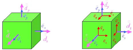
Fig. 2. Allocation of both electric grid voltages and electric grid

fluxes relative to a dual FIT cell. Left: before the interpolation. Right: after the interpolation.

half) through a B-type interpolation, building the voltage ˆ

ex(i−1/2, j+1/2, k).

The local interpolation process is expressed by the follow-ing equation:

ˆ

ex(i−1/2, j+1/2, k)=

1 4

ˆ

ex(i, j, k)

+ êx(i, j+1, k)+ êx(i−1, k, k)+ êx(i−1, j+1, k)

. (8)

Figure 2 shows the allocation of voltages relative to a dual cell after the interpolation (right-hand side) compared to the classical allocation (left-hand side).

To globally account the interpolation process, the follow-ing matrices are defined:

[Qx]pq=

1

2 p=q orp=q+1

0 else (9)

Qy_pq=

1

2 p=q orp=q+I

0 else (10)

Qz

pq=

₁

2p=qorp=q+I J

0 else , (11)

whereIandJ represent the maximum number of grid nodes in x- and y-directions, respectively (Kr¨uger, 2000). Within the FIT algorithm, the interpolation matrices will be placed at the off-diagonal terms in the material operator.

In order to keep the symmetry of the physical permittivity tensor the off-diagonal terms [Mε]u,vand [Mε]v,uof the

dis-crete material operator have to be equal. The symmetry of the material operator can be reached through the following steps:

– Assuming that primary and dual edges in the same di-rection have the same length, their cancellation leads to equal grid information in the above-mentioned terms of the material operator according to Eq. (12).

˜ Avw

Lv

= ˜ LvL˜w

Lv = ˜ Auw Lu = ˜ LuL˜w

Lu

≈ ˜Lw. (12)

The approximation introduced in Eq. (12) is given by Lu= ˜Lu+O(1), where the first order error term

(4)

Fig. 3. Construction of electric voltages on the grid.

Fig. 4. Top row: electric potential distribtuion. Bottom row: electric

flux density. Left column: εl/εp=1. Middle column: εl/εp=2.

Right column:εl/εp=3

– Averaging the permittivity along the common dual edge ˜

Lw resulting from the first step leads to equal material

information in the considered terms. The permittivity average for each off-diagonal term of the material oper-ator uses the approximation from Eq. (12):

RR

˜

Auwε dA+O(1

k+1₎

R

Luds+O(1

k₎ =

¯ ε ˜ Lw

R

˜

Luds

R

Luds

+O(1k)

≈ ¯ε ˜ Lw

+O(1

k∗₎_{≈ ¯}_ε ˜ Lw

, (13)

wherek∗_{∈ [}_1,₃_]_.

– Positioning the interpolation matrices within the mate-rial operator such as to ensure the symmetry regarding the interpolation process.

Table 1. Electric flux density (max value [C/m2]) given in % rela-tive to the max value in the case ofεl/εp=3.

εl/εp=1 εl/εp=2 εl/εp=3

dmax[C/m2] 13.5% 60.8% 100%

Taking into account the above considerations, the material operator becomes:

Mε=

   ˜ DAyzDεxxD

−1 Sx

QT_x Dεyx D˜Sz Qy

QT_x Dεzx D˜Sy Qz

QT_y DεxyD˜Sz Qx ˜

DAxzDεyyD −1 Sy

QT_y Dεzy D˜Sx Qz

QT_z DεxzD˜Sy Qx

QT_z DεyzD˜Sx Qy ˜

  .(14)

This distribution of the interpolation matrices to the off-diagonal terms ensures the global symmetry of the mate-rial operator. Due to the permittivity average, when cou-pling two directions the A-type interpolation is weighted with the length of a dual edge on the third direction. To keep the symmetry, the B-type interpolation cannot be length-weighted. Figure 3 shows that the voltageseˆy(i, j−1, k)and

ˆ

ey(i+1, j−1, k)are built along the dual edgeL˜z(i, j−1, k)

and the voltageseˆy(i, j, k),eˆy(i+1, j, k)are built along the

dual edgeL˜z(i, j, k).

6 Simulations

The human body model (HUGO) offered by the simulation software package CST EMStudio™ (CST GmbH) was used for the import of a cubic volume of muscle tissues within a C++ code where the anisotropic FIT was implemented. The diagonal direction of muscle fibres is described by the anglesφ=θ=45◦. These muscles were placed in the elec-trostatic field determined by the imposed potential values of −10 V and+10 V, at the boundary planes Z=min and Z=max, through the Dirichlet boundary conditions. All the other boundaries, were treated with Neumann boundary con-ditions. Three simulations were performed using the CG solver from PETSc (Balay et al., 1997) corresponding to three different values for the ratio between longitudinal and perpendicular permittivity of muscle tissues with respect to their fibre direction, i.e.εl/εp=1;2;3.

7 Results and discussions

In Fig. 4, the top row presents three scalar plots of the electric potentials computed inside a muscle volume considered to be isotropic (left), anisotropic (having the ratioεl/εp=2

(mid-dle)) and anisotropic (withεl/εp=3 (right)). Comparing the

(5)

The bottom row in Fig. 4 presents three vector plots of the electric flux density, each computed with the correspond-ing electric potentials in the same column and scaled to the same maximum value which was found in the anisotropic case ofεl/εp=3. Relative to this value, the other maximum

values are given in percentage in Table 1. Compared to the isotropic case where the electric flux is homogeneous in the entire muscle volume, in the anisotropic cases, the flux has higher values along the fiber’s direction.

8 Conclusions

In this paper we presented the anisotropy of muscle tissues with regard to dielectric permittivity and its mathematical an-alytic model. This model was further discretized to conform with the numerical algorithm of the Finite Integration Tech-nique and implemented in software code. With this code, more simulations were performed and the results were com-pared to the isotropic case.

Acknowledgements. The authors are grateful to M. Clemens (TU

Darmstadt) for many useful suggestions as well as to F. Sachse (IBT Karlsruhe, now CVRTI Univ. of Utah) for providing us with the Orientation Data Set. V. Motrescu was supported by DFG (RI 814/12-1) and CST GmbH, Darmstadt.

References

Balay, S., Gropp, W. D., McInnes, L. C., and Smith, B. F.: PETSc – Efficient Management of Parallelism in Object Oriented Nu-merical Software Libraries, Modern Software Tools in Scientific Computing, 163–202, Birkhauser Press, 1997.

CST EMStudio™: CST GmbH, Bad Neuheimer Str. 19, D-64289, Darmstadt, Germany.

Durney, C. H., Massoudi, C. H., and Iskander, M. F.: Radiofre-quency Radiation Dosimetry Handbook, Fourth Edition, Univ. of Utah, Salt Lake City, http://www.brooks.af.mil/AFRL/HED/ hedr/reports/handbook/home.html, 1986.

Gabriel, S., Lau, R. W., and Gabriel, C.: The dielectric properties of biological tissues: II. Measurements in the frequency range 10 Hz to 20 GHz, Phys. Med. Biol., 41, 2251–2269, 1996. Kr¨uger, H.: Zur numerischen Berechnung transienter

elektromag-netischer Felder in gyrotropen Materialien, Dissertation, Tech-nische Universit¨at, Darmstadt, 2000.

Sachse, F. B., Werner, C., Mueller, M., and Meyer-Waarden, K.: Preprocessing of the Visible Man dataset for the generation of macroscopic anatomical models, Proc. First Users Conference of the National Library of Medicine’s Visible Human Project, 123–124, 1996a.

Sachse, F. B., Werner, C., Mueller, M., and Meyer-Waarden, K.: Segmentation and tissue-classification of the Visible Man dataset using the computer tomographic scans and the thin sections pho-tos, Proc. First Users Conference of the National Library of Medicine’s Visible Human Project, 125–126, 1996b.

Sachse, F. B., Werner, C., Meyer-Waarden, K., and D¨ossel, O.: Comparison of Solutions to the Forward Problem in Electro-physiology with Homogeneous, Heterogeneous and Anisotropic Impedance Models, Biomedizinische Technik, 42, 277–280, 1997.

Sachse, F. B., Wolf, M., Werner, C., and Meyer-Waarden, K.: Extension of Anatomical Models of the Human Body: Three-Dimensional Interpolation of Muscle Fiber Orientation Based on Restrictions, J. Computing and Information Technology, 6, 1, 95–101, 1998.

van Rienen, U., Flehr, J., Schreiber, U., and Motrescu, V.: Mod-eling and Simulation of Electro-Quasistatic Fields, ModMod-eling, Simulation and Optimization of Integrated Circuits, Interna-tional Series of Numerical Mathematics, Birkh¨auser Verlag Basel/Switzerland, 146, 17–31, 2003.

van Rienen, U.: Numerical Methods in Computational Electrody-namics – Linear Systems in Practical Applications, Springer-LNCSE, Verlag Berlin Heidelberg, 12, 2001.