1Computational Aerodynamics
Institute, China Aerodynamics Research and Development Center, Mianyang 621000, China Full list of author information is available at the end of the article
Abstract
This paper presents an engineering-oriented UGKS solver package developed in China Aerodynamics Research and Development Center (CARDC). The solver is programmed in Fortran language and uses structured body-fitted mesh, aiming for predicting aerodynamic and aerothermodynamics characteristics in flows covering various regimes on complex three-dimensional configurations. The conservative discrete ordinate method and implicit implementation are incorporated. Meanwhile, a local mesh refinement technique in the velocity space is developed. The parallel strategies include MPI and OpenMP. Test cases include a wedge, a cylinder, a 2D blunt cone, a sphere, and a X38-like vehicle. Good agreements with experimental or DSMC results have been achieved.
Keywords:Unified gas kinetic scheme, Conservative discrete ordinate method, Implicit algorithm, Mesh refinement, MPI, OpenMP, Application
1 Introduction
During the reentry process, vehicles may encounter different flow regimes such as free molecular, transitional, near continuum, and continuum regime. The determination of aerodynamic forces and heat loads has great impact on the design of vehicles [1]. In the non-continuum regimes, traditional macroscopic methods, such as Euler, Navier-Stokes and Burnett equations, may become invalid. The following methods are mainly used for the non-equilibrium flow simulations. The first kind of method is based on probabilistic modeling. The most popular one is the direct simulation Monte
Carlo (DSMC) method. DSMC was first proposed by Bird [2] more than half a century
ago. It follows the evolution of representative particles with uncoupled transport and collision process. The DSMC has been fully validated for providing physical solutions through its comparison with the experiments measurements [3,4]. It has played a key role in the design and flight analysis of vehicles in the rarefied environment. Some of
the most cited DSMC codes in literature are DS2V/3 V [5], DAC [6], SMILE [7],
MONACO [8], and DSMCFOAM [9]. The main differences among these codes are in
the treatment of collision selection methods and mesh topology.
Another kind of approach is the deterministic method. Deterministic method mainly concerns the Boltzmann equation. Due to the complexity of the Boltzmann collision term, researchers usually choose the simplified collision model, such as BGK model [10], Shakhov model [11], Rykov model [12]. Titarev [13] has developed an implicit
solver named Nesvetay-3D on unstructured mesh. Three-dimensional TVD method is applied for the numerical discretization. Both spatial and velocity mesh decomposition
are used in the parallelization. A total number of 6.9 × 10⁹ mesh points in the
six-dimensional space is used for the supersonic flow simulation around a re-entry space vehicle. Wadsworth [14] has developed a parallel, finite volume 2D/axisymmetric code SMOKE which is based on conservative numerical schemes developed by Mieus-sens [15]. In Baranger’s team, a 3D code [16] has been used in the past years for rar-efied flow simulations. This code can handle polyatomic gases. It uses block structured mesh and hybrid parallelization, i.e., space domain decomposition with MPI and inner parallelization with OpenMP. Furthermore, the code is equipped with velocity mesh re-finement technique which improves the code in both CPU time saving and memory
storage. Li’s team has developed a 3D code based on the model equation with the name
gas-kinetic unified algorithm (GKUA) [17, 18]. Three-dimensional hypersonic flows
around sphere and spacecraft with different Knudsen numbers and Mach numbers have been studied. The total six-dimensional mesh for a complex wing-body configur-ation reaches 7.3 × 10¹¹and 23,800 CPU cores [19] have been used in the computation. However, the above deterministic methods share a common feature. They decouple the particle transport and collision. Therefore, the cell size and time step in these numerical schemes are limited by the particle mean free path and mean collision time in order to provide accurate numerical solutions. When the flow regime is close to continuum or near continuum, the time step and cell size limitations are rather severe and make these methods extremely time-consuming and inefficient.
Another distinguishable deterministic method, which is named unified gas kinetic
scheme (UGKS), was proposed by Xu et al. [20–22]. UGKS is a multi-scale method
with coupled particle transport and collision in its numerical flux modeling. It is based on an integral solution of the gas-kinetic model equation. It can recover the flow phys-ics from the kinetic particle transport and collision to the hydrodynamic wave propaga-tion. Moreover, the time step is determined only by the CFL condition, which is not limited by the mean collision time. So the scheme becomes more efficient in various flow regimes, especially when the local Knudsen number is low. Applying UGKS to analyze aerodynamic and aerothermodynamics on flying vehicles in near space flight is our long term objective.
This paper is organized in the following. Section2is about the introduction of UGKS and some techniques to accelerate convergence. Section3is a simple description of the
framework. Section 4 is some 2D and 3D validation test cases. The last section is the
conclusion.
2 Method
2.1 Unified gas kinetic scheme
The three-dimensional Shakhov model equation [11],which can give the correct Prandtl
number, in non-dimensional form reads
ftþufxþvfyþwfz¼ f þ−f
τ ð1Þ
where the free-stream parameters density ρ∞, velocity U∞, viscosity coefficient μ∞ and
and ! ¼c !u−!U is the peculiar velocity. T, !q, Pr are the temperature, heat flux and Prandtl number, respectively.
The relations between conservative variables ρ, ρU, ρV,ρW, ρE with the probability density function is
ρ;ρU;ρV;ρW;ρE
ð ÞT¼
Z
ψTfdΞ ð2Þ
where ψT= (1,u,v,w, 1/2(u2+v2+w2))T is vector of moments anddΞ=dudvdwis the volume element in the phase space.
Integrating Eq. (1) in the volume element we can get
∂Q
∂t þ
∂F
∂xþ
∂G
∂y þ
∂H
∂y ¼0 F¼
Z
ufψαdΞ G¼
Z
vfψαdΞ H¼
Z
wfψαdΞ
ð3Þ
where the conservation constraint or compatibility condition in the following form has been used
Z
f−fþ
ψαdΞ¼0 ; α¼1;2;3;4;5 ð4Þ
For curvilinear coordinate system, applying the finite volume method eq. (3) goes to
ΔQ¼−V−1
Z tnþ1
tn
JS
ð Þiþ1=2;j;k−ðJSÞi−1=2;j;k
þðJSÞi;jþ1=2;k−ðJSÞi;j−1=2;k
þðJSÞi;j;kþ1=2−ðJSÞi;j;k−1=2 2
4
3 5dt
J¼FiþGjþHk
ð5Þ
where V is the cell volume, S and J are the cell face vectors and flux vectors, respectively.
The flux across a cell interface is based on the integral solution of the model equa-tion. Discontinuous spatial reconstruction with nonlinear limiter is used to introduce artificial dissipation for UGKS once the scheme becomes a shock capturing method when the dissipative flow structure cannot be well resolved by the cell size. Details can be found in [20]. In this paper, we use van Leer limiter in the reconstruction. Due to the discreteness of the velocity space, numerical quadrature should be used to calculate various integrals. In this paper, composite Newton-Cote’s (N−C) quadrature is adopted.
The Rykov model [12] for diatomic gases is also implemented in our UGKS code
2.2 Conservative discrete ordinate method [23]
The compatibility condition Eq. (4) is the basis for the governing Eq. (3). But once the
DOM is introduced and the velocity space is discretised, Eq. (4) no longer holds and
becomes Z
f−fþ
ψαdΞ¼ErrðN−CÞ ð6Þ
Here Erris the numerical error introduced by the numerical quadrature.Errcan be
reduced by increasing the velocity space mesh in a certain extent but will finally stay in some level, which is determined by the intrinsic nature of numerical quadrature.
This numerical error results in a source term in the governing Eq. (5). The source
term can be expressed in the formRttζζþ1½1τErrðN−CÞdt Define
SS¼ 1
Δt
Z tζþ1
tζ 1
τErrðN−CÞ
dt≈ 1
τErrðN−CÞ
ζþ1
ð7Þ
HereΔtis the marching time step. The five components ofSScorrespond to the
gov-erning equations of mass, momentum in the x, y and z directions and the energy, re-spectively. After some simple derivations we can get
τ¼ μ
pRe∞∝ Kn∞
M∞ μ
p ð8Þ
From Eq. (7) and Eq. (8) we can see that SSis related to free-stream condition and numerical quadrature.
In order to eliminate the numerical source term completely, we introduce CDOM proposed by Titarev [24] into UGKS,
∭fþ−f
τ ψT1dudvdw¼
1
τ 0;0;0;0;0;−2=3qx;−2=3qy;−2=3qz
T
ð9Þ
where
ψT
1 ¼ 1;u;v;w;
1 2 u
2þv2þw2
;1
2ðu−UÞc
!2
;1
2ðv−VÞc
!2
;1
2ðw−WÞc
!2
T
c
!2
¼ðu−UÞ2þðv−VÞ2þðw−WÞ2
The first five equations in (9) represent conservation of mass, momentum and energy during collision process. In discretised velocity space, the multiple integral is replaced by numerical quadratures. If the equilibrium distribution function remains in the form given in section 2.1, Eq. (9) no longer holds due to numerical error of quadratures. In other words, the conservation property will not be maintained.
Substituting the expression ∭fψT
1dudvdw¼ ðρ;ρU;ρV;ρW;ρE;qx;qy;qzÞ
T
into Eq. (9) we can get a new Eq. (10), which can be solved by the Newton iteration method. An initial guess equals to (ρ,U,V,W,λ,qx,qy,qz) is provided. Then a new group of variables,ðρ0;U0;
V0;W0;λ0;qx0;q0y;q0zÞcan be got.
numerical source term Errgoes to machine zero, which has been validated in numer-ical experiments.
The UGKS in Section2.1has a second-order of accuracy. What we do in this section
only changes the form of the heat flux modified equilibrium state. The spatial recon-struction and the evaluation of the numerical flux remain unchanged. Thus, CDOM does not affect the spatial accuracy and the coupling of particle transport and collision.
2.3 Implicit UGKS [25]
The governing equation in a physical control volume (i,j,k), at velocity mesh point
ul, m, n= (ul,vm,wn), is given by
∂fi;j;k;l;m;n ∂t þul
∂fi;j;k;l;m;n ∂x þvm
∂fi;j;k;l;m;n ∂y þwn
∂fi;j;k;l;m;n ∂z ¼
fþi;j;k;l;m;n−fi;j;k;l;m;n
τ ð11Þ
DefineΔf=fζ+ 1−fζandΔt=tζ+ 1−tζ, then the implicit method reads
1þΔt 1
τζþΔtul;m;n∇
Δf
ð Þi;j;k;l;m;n¼ΔtR
ζ
i;j;k;l;m;n
Rζi;j;k;l;m;n¼−ul
∂fζi;j;k;l;m;n
∂x −vm
∂fζi;j;k;l;m;n
∂y −wn
∂fζi;j;k;l;m;n
∂z þ 1 τζ fþ−f
¼−R0þ 1 τζ fþ−f
ð12Þ
whereR'is the evolving time averaged flux which can be written as
R0¼
RΔtt
0 X6
ii¼1
unfpð Þt dt
Δtt ð13Þ
whereun=ul,m,n•niiandniiis the unit vector normal to the cell interface. The evolving time step Δtt is different from the marching time step Δt. Based on some numerical experimental results, we propose in this paper the following principle to determineΔtt
Δtt<Δtmin=CFL ð14Þ
whereΔtminis the minimum time step in the whole field determined by the CFL condition. Eq. (12) can be rewritten in the following form
1þΔt 1
τζ
Δf
ð Þi;j;k;l;m;nþ
Δt Vi;j;k
X6
ii¼1
ul;m;nnii
Si;j;k;iiFF ð ÞiΔf ;j;k;l;m;n;ð ÞiΔf 1;j1;k1;l;m;n
¼ΔtRζi;j;k;l;m;n
where the subscripts (i1,j1,k1) indicates the cell sharing the iith edge with the (i,j,k) cell. The quantity FFcan be expressed as
FF ð ÞΔf i;j;k;l;m;n;ð ÞΔf i1;j1;k1;l;m;n
¼1
2 ð ÞΔf i;j;k;l;m;nþð ÞΔf i1;j1;k1;l;m;n
h i
þ1
2 sign ul;m;nnii
Δf
ð Þi;j;k;l;m;n−ð ÞΔf i1;j1;k1;l;m;n
h i
Substituting the above expression into Eq. (15) we can get
Fig. 2Distribution function at pts4
Fig. 1Temperature contour for the jet case
1þΔt1
τζþΔtbi;j;k;l;m;n
Δf
ð Þi;j;k;l;m;nþ
X6
ii¼1
Δtci;j;k;l;m;nð ÞΔf i1;j1;k1;l;m;n¼ΔtRζi;j;k;l;m;n
bi;j;k;l;m;n¼
X6
ii¼1
ul;m;nnii
1þ sign ul;m;nnii
Si;j;k;ii
2Vi;j;k
ci;j;k;l;m;n¼ ul;m;nnii
1−sign ul;m;nnii
Si;j;k;ii
2Vi;j;k
ð16Þ
Writing Eq. (16) in matrix form
IþΔtZl;m;n
ð ÞΔf l;m;n¼ΔtΧl−;1m;nRζl;m;n ð17Þ
Δf
ð Þl;m;n¼
Δf
ð Þ1;1;1;l;m;n
Δf
ð Þ2;1;1;l;m;n
⋯
Δf
ð ÞNI−1;NJ−1;NK−1;l;m;n
0 B B @ 1 C C
A Rζl;m;n¼
Rζ1;1;1;l;m;n Rζ2;1;1;l;m;n
⋯
RζNI−1;NJ−1;NK−1;l;m;n
0 B B B @ 1 C C C A
Χl;m;n¼
χ1;1;1;l;m;n 0 ⋯ 0
0 χ2;1;1;l;m;n ⋯ 0
0 0 ⋯ 0
0 0 ⋯ χNI−1;NJ−1;NK−1;l;m;n
0 B B @ 1 C C A
Table 1Free-stream conditions
Configuration Mach Kn λdefinition Working gas L(m) ω T∞(K) Tw(K)
Wedge 10 0.05 HS Argon 0.2 0.81 200 300
Cylinder 1.96 0.0162, 0.162 VHS Nitrogen radius 0.74 124.94 259.87
Cylinder 5 0.01, 0.1, 1 VHS Argon radius 0.81 273 273
Cylinder 10 3.03e-3, 7.58e-2 VHS Argon radius 0.81 200 500
Cylinder 25 3.69e-3, 1.84e-2 9.22e-2, 0.461
VHS Argon radius 0.734 200 1500
Cone 8.1 9.75e-3, 3.38e-1 VHS Argon 0.02 0.81 247, 189 273
Sphere 4.25 0.031~0.672 VHS Nitrogen 0.002 0.74 65 302
Sphere 5.45 0.256~1.96 VHS Nitrogen 0.002 0.74 43 315
X38-like 4 8.41e-5~8.41e-2 VHS Argon 0.28 0.81 56 300
X38-like 6 1.26e-4~1.26e-1 VHS Argon 0.28 0.81 56 300
X38-like 8 1.68e-4~1.68e-1 VHS Argon 0.28 0.81 56 300
where NI, NJ and NK are the physical mesh points in the i, j and k directions, respectively.
Applying approximate LU decomposition to (I+Δt⋅Zl,m,n) we can get
IþΔtZl;m;n¼Ll;m;nUl;m;nþ◯ Δt2
WhereLl,m,nandUl,m,nare both diagonal matrices and can be given by
lpq ¼ Δtzpq p<q
0 p>q
upq ¼
0 p<q
Δtzpq p>q
lpp¼upp¼1
The implicit method in the final form reads
Ll;m;nUl;m;nð ÞΔf l;m;n¼ΔtΧl−;1m;nR
ζ
l;m;n ð18Þ
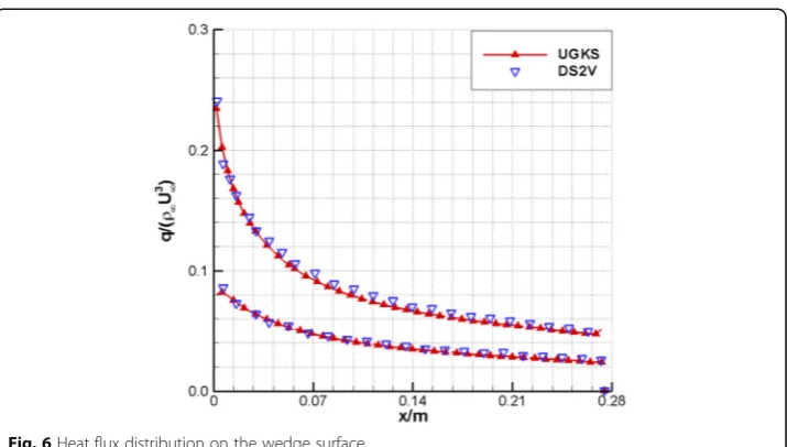
Fig. 5Pressure distribution on the wedge surface
Fig. 4Pressure contour of the wedge
In structured meshes, (Δf)l,m,ncan be obtained after backward and forward
substitu-tion andfζ+ 1can be got subsequently.
In the above procedure, the gain term f+ in the collision term is treated explicitly. Since UGKS is a multi-scale hybrid method with both macroscopic and microscopic variable updates. The macroscopic variables can be updated implicitly first to give a pre-evaluatingf+, resulting in a complete implicit implementation [26] for the collision term. This is very useful for continuum or near continuum flows.
2.4 Local refinement in the velocity mesh
Generic adaptive mesh refinement (AMR) [27,28] in velocity can greatly decrease the CPU time and memory requirements for UGKS. However, the resulting velocity meshes are usually different for different spatial cells, making it rather difficult to apply the im-plicit technique.
Fig. 7Shear stress distribution on the wedge surface
In our UGKS solver package, we combine the merits of both methods through the following procedure. First, the bounds and interval of a global uniform velocity mesh are calculated according to numerical experiences or a pre-conducted Navier-Stokes simulation results. Obviously, the lower and upper limits of the velocity mesh in each direction are determined by the highest temperature which usually appears in the shock
layer. While the mesh intervalΔvis determined by the lowest temperature in the whole
field. Second, a global uniform velocity mesh is generated which we call background
mesh. The interval of this mesh is a•Δvwhere a is larger than one. Then we give a
patch on the background velocity mesh for the spatial cells whose velocity mesh
inter-val should be less than a•Δv. The location of the patch can be determined by the
pre-calculated Navier-Stokes results or even by the UGKS results with the background velocity mesh. The resulting velocity mesh is still structured. The implicit method can be applied without any difficulties.
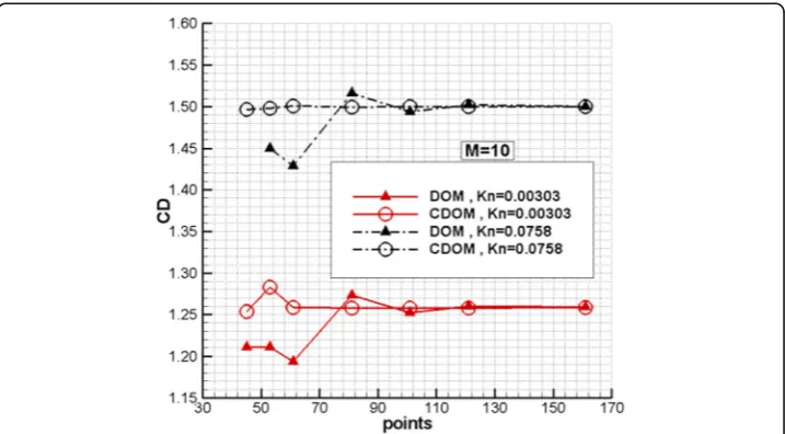
Fig. 9Cylinder drag coefficient vs points in u(v) direction
Fig. 8|SS(1)| on the cylinder surface
Up to now, the only difficulty arising may be the interpolation of distribution func-tions from the background mesh to the patch. We use the following conservative
method. Take 1D case for example, the composite Newton-Cote’s quadrature requires
that the total number of velocity points is 4 N + 1, where N is a positive integer. We can get an interpolation polynomial from the five distribution functions which is equally spaced on a small block of four successive intervals on the velocity mesh. Since
Newton-Cote’s quadrature coefficients are derived from this polynomial, they are
consistent. It can be easily proved that the conservations of mass, momentum and energy hold if we extend the original 5 points equally spaced mesh to a 9 points equally spaced mesh. For 2D or 3D cases, extending a block mesh of 5 × 5 or 5 × 5 × 5 to 9 × 9 or 9 × 9 × 9 can be done in the same way. Proof of the conservation law can be verificated through some mathematical software such as MAPLE.
We have applied this technique in a 2D jet case on a blunt cone. The freestream
Mach number is 8.1 with an altitude of 90 km. The jet condition is ρj= 7.468e−3,
Fig. 10Convergent histories of the drag coefficient with Ma = 5.0 and Kn = 0.01
uj=cj, pj= 373Pa, Tj= 240K. The pressure ratio of the jet to the free-stream is
about 2000. For the jet-off case, a velocity mesh of 121 × 121 is enough. For the jet-on case, the local temperature decreases severely due to rapid expansion from
the jet exit. Figure 1 shows the temperature contour. The temperature in the
downstream of the jet near pts4 is about one order lower than the free-stream temperature. Thus, it’s necessary to refine the velocity mesh in order to resolve the corresponding distribution function. From the pre-conducted UGKS results, we choose 9 blocks of 5 × 5 sub-mesh and extend them to 9 × 9 sub-mesh. The final
distribution function and the velocity mesh are shown in Fig. 2.
In this case, if we use global uniform mesh, the total mesh will be 241 × 241. With the local refinement technique, the total mesh is 121 × 121 + 9 × (9 × 9 - 5 × 5) = 15,145 which is only 1/3.8 of the former.
2.5 Parallelization
At present, hybrid parallelization similar to that in [16] is used. The space mesh is decomposed and parallelized with MPI which has been broadly applied in many trad-itional CFD software. In every MPI process, several threads are used with OpenMP. However, due to the architecture change of our new super cluster, three space dimen-sions and one velocity dimension decomposition technique is under developing, allow-ing for a larger parallel scale up to 10,000 cores in the near future.
3 Code framework
The UGKS solver package is based on the framework of our in-house NS solver,
CARDC Hypersonic Aerodynamic Numerical Tunnel (CHANT) [29]. Figure 3 shows
Table 2Comparison of the explicit and implicit methods in convergence rate
Ma Kn Nc.E Nc.I Rs = Nc.E/ Nc.I/1.02
5 0.01 502,450 5800 84.93
5 0.1 463,500 3500 129.83
10 0.01 505,900 4645 106.78
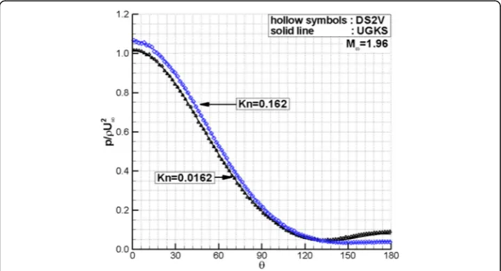
Fig. 12Pressure distributions on the cylinder surface at M = 1.96
the general sketch. The whole package is composed of five parts: input, output, initialization, control and calculation. The flowfield of a certain configuration is ob-tained through calculations over all structured blocks one by one. Multi-stage interface is devised for further development. Fortran90 is used for all subroutines.
The current features of UGKS solver package can be summarized as follows:
2D and 3D body-fitted structured multi-block mesh Steady and unsteady simulations
Explicit and implicit methods
Conservative discrete ordinate method Local refinement in velocity mesh Shakhov model for monatomic gases Rykov model for diatomic gases
Fig. 13Slip velocity distributions on the cylinder surface at M = 1.96
Diffuse or specular reflection wall boundaries, free-stream boundary, outflow boundary, symmetrical boundary
Several models for the viscosity calculation such as hard sphere model, variable hard sphere model [30] or the Sutherland model
Hybrid parallelization with MPI and OpenMP
4 Validation cases
Five test cases are considered. UGKS results are compared with those obtained from
either DS2V [5], MONACO [31], RariHV [32] or experiments. Fully diffuse solid
boundary is used. In all cases, the global Knudsen number Kn is defined as
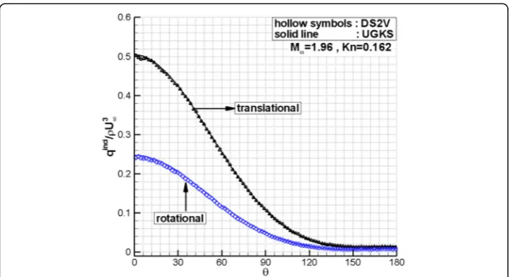
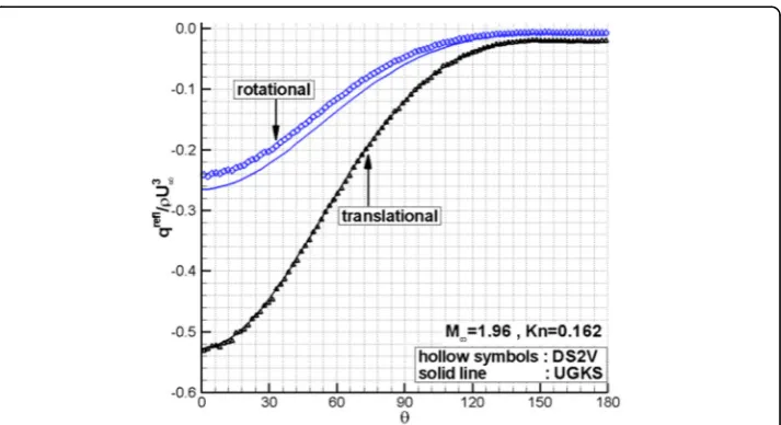
Fig. 15Reflective heat flux distributions on the cylinder surface at M = 1.96
Fig. 16Pressure distributions on the cylinder surface at M = 5
Kn¼λ
L ð19Þ
where λ is the mean free path which is determined for either hard sphere (HS) mole-cules [30].
λ¼16
5
ffiffiffiffiffiffiffiffiffiffiffi
m 2πkT
r
μ
ρ ð20Þ
or variable hard sphere (VHS) molecules
λ¼2 5ð −2ωÞð7−2ωÞ
15
ffiffiffiffiffiffiffiffiffiffiffi
m 2πkT
r
μ
ρ ð21Þ
where ω is the power law index of the viscosity, m is the atomic mass, k is the Boltzmann constant.
Fig. 17Heat flux distributions on the cylinder surface at M = 5
The main free-stream conditions for all cases are summarized in Table1.
4.1 Hypersonic flow over a 400wedge
The angle of attack is 10 degrees. Figure 4 shows the pressure contour predicted by
UGKS. Figures 5,6 and 7 display the pressure, heat flux and shear stress distributions on the surface, respectively. The UGKS results and DS2V results are almost identical, indicating that UGKS code package and DS2V can predict flows with similar accuracy.
4.2 Super and hypersonic flows over a 2D cylinder
This is a quite comprehensive test case covering supersonic and hypersonic flows in all regimes. We also use this case for validating the CDOM and implicit techniques de-scribed in section2.
Fig. 19Shear stress distributions on the cylinder surface at M = 10
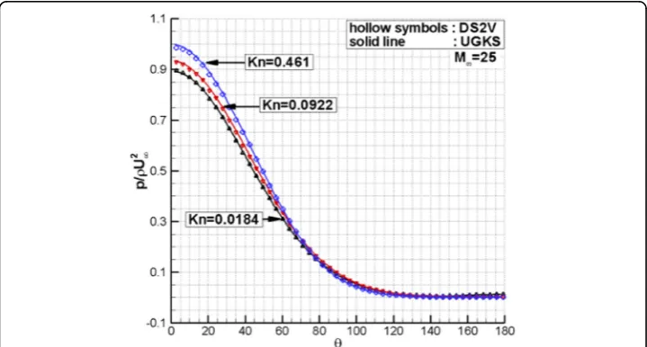
Fig. 20Pressure distributions on the cylinder surface at M = 25
For Mach number 10, both DOM and CDOM calculations are conducted. Figure 8
shows the variable |SS(1)| in the cells just near the wall at different velocity space meshes. When the velocity space mesh increases, the numerical source term decreases but will stay at a certain level finally. So increasing the velocity space mesh will not elimin-ate the source term. However, the source term will be on an order of 10−14~10−15 if CDOM is applied. The total drag at different velocity space meshes is given in Fig.9. Ob-viously, the mesh dependence with CDOM is much smaller than that with DOM. The so-lution at 61 × 61 mesh with CDOM can be considered as mesh convergent while with DOM the same result can only be obtained at a much finer mesh of 121 × 121. Thus, the time and memory cost will decrease by nearly three quarters with the help of CDOM.
Figures 10and 11show the convergent histories of the drag coefficient and residual
for Mach number 5 and Knudsen number 0.01, respectively. A comparison of the
expli-cit and impliexpli-cit methods in convergence rate is shown in Table 2. Nc.E and Nc.I are
the total iterations steps for a convergent solution for the explicit and implicit methods,
Fig. 21Heat flux distributions on the cylinder surface at M = 25
Table 3Comparisons of cylinder drag
M∞ Kn∞ UGKS DS2V/MONACO Relative error (%)
1.96 0.0162 1.597 1.582 0.92
1.96 0.162 1.862 1.863 −0.06
5 0.01 1.320 1.316 0.31
5 0.1 1.527 1.523 0.28
5 1 1.929 1.917 0.62
5.43 0.303 1.774 1.775 −0.05
5.43 1.52 2.277 2.304 −1.19
10 0.00303 1.258 1.252 0.56
10 0.0758 1.500 1.496 0.27
25 0.00369 1.256 N-A/1.259 −0.21
25 0.0184 1.348 1.349/1.347 0.07
25 0.0922 1.531 1.521/1.528 0.22
respectively. Rs is the speed-up ratio for the implicit method, where the denominator 1.02 comes from the fact that the computational cost of one time step for the implicit method is about 2% more than that for the explicit method. A speed up ratio of nearly two orders can be achieved.
Figures 12,13,14and 15show the comparisons between UGKS and DS2V for a
di-atomic nitrogen gas. The UGKS results are obtained with the Rykov model with rota-tional degrees of freedom. Thus, the heat flux can be divided into two parts, the contributions of translational degree and rotational degree. Good agreements can be seen, providing a sound validation for our UGKS code for diatomic gases.
Figures 16and 17are the results for Mach number 5. Figures18and 19are the
re-sults for Mach number 10. Figures20and21are the results for Mach number 25. We
omit some comparisons at certain Mach numbers because of space limitations.
Table 3 gives the drag coefficient comparisons. The maximum relative error is only
2.03%.
Fig. 23Pressure contour and streamlines
Fig. 22Cone model
4.3 Hypersonic flow over a 2D cone
Figure 22gives the computational configuration. The angle of attack is 0 degree. The
pressure contour and streamlines are shown in Fig.23. The altitude in the figure is only
‘nominal’ which means that only the temperature and number density at the
corre-sponding altitude are used, since the air is treated as a monatomic gas. In other words,
internal degrees of freedom are ignored. The two global Knudsen numbers in Table 1
for cone case correspond to nominal altitudes 60 km and 85 km, respectively. The flow pattern is relatively simple, i.e., a bow shock in front of the blunt body and a vortex in the bottom similar to that in a backward step case. However, the bow shock in front of the 85 km case is much weaker than that in the 60 km case. The recirculation zone in the bottom is smaller, too.
Figures 24,25and 26show the pressure, heat flux, and shear stress distributions on the cone surface, respectively. The abscissa indicates the distance from the very begin of the cone on the surface. The bottom pressure at 60 km rises about one order from the corner to the center of the bottom, resulting in a large adverse pressure gradient and inducing a large separation. At 85 km, the pressure curve is rather flat and only
a
b
Fig. 25Heat flux distributions on the cone surface (a) Body (b) Bottom
small adverse pressure gradient occurs. Moreover, the minimum pressure, heat flux and stress at the bottom are almost three orders lower than the maximum values on the cone. UGKS can capture these phenomena as accurately as the DS2V.
4.4 Supersonic and hypersonic flows over a sphere
The flow past a sphere is simulated with Rykov model to compare with the experimen-tal drag coefficients [33]. The space mesh contains 21,840 cells while a velocity mesh of 41 × 41 × 41 is used.
Figure 27shows the pressure contour for two cases. When the Knudsen number is
large, variable gradient in the whole field is small. There is only weak compressive wave in front of the sphere.
a
b
Fig. 27Pressure contour on the symmetry plane and the sphere surface (a) M = 4.25, Kn = 0.031 (b) M = 5.45, Kn = 1.96
a
b
Fig. 26Shear stress distributions on the cone surface (a) Body (b) Bottom
Table 4 gives the drag coefficient comparisons. The maximum relative error is only 2.64%. The agreements can be considered as excellent since the root mean square (RMS) error of the experiments is about ±2%.
4.5 Supersonic and hypersonic flows over a X38-like vehicle
The angle of attack is 20 degrees in this case. The space mesh contains 334,434 cells while a velocity mesh of 33 × 33 × 33 is used. The total six-dimensional mesh reaches 1.2 × 10¹⁰. The reference area for the aerodynamic coefficient is 2.41 × 10⁻²m2.
Figure 28 gives the spatial streamlines around the vehicle with Mach number 4.
When the free-stream Knudsen number is relatively small, the adverse pressure gradi-ent can be large enough to induce the flow to separate from the boundary, resulting in the vortex in Fig.28(a).
Figure29shows the local Knudsen number distribution near the surface. Local Knudsen number is calculated through Eq. (19) with the characteristic length L substituted by the local gradient-length Q/|dQ/dl| proposed by Boyd [34]. In this paper, the density-based gradient-length is used. The local Knudsen number can cover a wide range of values with
5.45 16.8 0.490 2.248 2.28 1.41%
5.45 32.1 0.256 2.005 2.04 1.71%
a
b
four to five order of magnitude difference. Thus, such a multi-scale method as UGKS is needed in order to correctly simulate these flow fields.
Table 5 gives the aerodynamic coefficients comparisons for Mach number 8. The
DSMC results are provided with RariHV which is an in-house DSMC software based on unstructured mesh in our group. The maximum relative error is only 2.27%.
5 Conclusions
Our UGKS solver package is introduced including the main numerical techniques for improving the efficiency and accuracy, such as implicit method and local mesh refine-ment technique in the velocity space. It is devised for simulating flow fields around complex configurations for all flow regimes.
Several validations are conducted by comprehensive comparisons with industry-standard DSMC code and experimental results including the pressure, heat flux, shear stress and aerodynamic coefficients for supersonic and hypersonic flows at almost all regimes. The agreements are satisfactory in all cases.
Future work include more application to 3D complex configurations and complex flow, improvement on physical models to consider vibrational degree, implementation of models for gas mixtures, and increases in computational efficiency and accuracy.
a
b
Fig. 29Local Knudsen number distribution (a) M = 6, Kn = 1.26e-4 (b) M = 6, Kn = 1.26e-2
Table 5Comparisons of X38-like coefficients with Mach number 8
Coefficients Kn UGKS RariHV Relative error(%)
Lift 1.68e-1 1.98E-01 1.96E-01 0.98
1.68e-2 1.94E-01 1.92E-01 1.15
1.68e-3 1.93E-01 1.94E-01 −0.69
Drag 1.68e-1 1.00E+ 00 9.79E-01 2.27
1.68e-2 5.56E-01 5.46E-01 1.85
1.68e-3 2.90E-01 2.95E-01 −1.71
Competing interests
The authors declare that they have no competing interests.
Publisher’s Note
Springer Nature remains neutral with regard to jurisdictional claims in published maps and institutional affiliations.
Author details
1Computational Aerodynamics Institute, China Aerodynamics Research and Development Center, Mianyang 621000,
China.2National University of Defense Technology, Changsha 410000, China.
Received: 17 January 2019 Accepted: 22 January 2019
References
1. Ivanov MS, Gimelshein SF (1998) Computational hypersonic rarefied flows. Annu Rev Fluid Mech 30:469–505 2. Bird GA (1963) Approach to translational equilibrium in a rigid sphere gas. Phys Fluids 6(10):1518–1519 3. Bird GA (1990) Application of the direct simulation Monte Carlo method to the full shuttle geometry. AIAA
Paper 90–1692
4. Pham-Van-Diep G, Erwin D, Muntz EP (1989) Nonequilibrium molecular motion in a hypersonic shock wave. Science 245:624–626
5. Bird GA (2005) The DS2V/3V program suite for DSMC calculations. Rarefied Gas Dynamics. Amer Inst Physics, Melville, 541–546
6. LeBeau GJ (1999) A parallel implementation of the direct simulation Monte Carlo method. Comput Methods Appl Mech Eng 174:319–337
7. Ivanov MS, Markelov GN, Gimelshein SF (1998) Statistical simulation of reactive rarefied flows: numerical approach and applications. AIAA Paper 98–2669
8. Dietrich S, Boyd ID (1996) Scalar and parallel optimized implementation of the direct simulation Monte Carlo method. J Comput Phys 126(2):328–342
9. Scanlon TJ et al (2010) An open source, parallel DSMC code for rarefied gas flows in arbitrary geometries. Comput Fluids 39(10):2078–2089
10. Bhatnagar PL, Gross EP, Krook M (1954) A model for collision processes in gases I: small amplitude processes in charged and neutral onecomponent systems. Phys Rev 94(3):511–525
11. Shakhov E (1968) Generalization of the Krook kinetic equation. Fluid Dynamics 3(5):95–96
12. Rykov VA (1975) A model kinetic equation for a gas with rotational degrees of freedom. Fluid Dynamics 10(6):959–966 13. Titarev V, Dumbser M, Utyuzhnikov S (2014) Construction and comparison of parallel implicit kinetic solvers in three
spatial dimensions. J Comput Phys 256:17–33
14. Wadsworth DC et al (2009) Assessment of Translational Anisotropy in Rarefied Flows Using Kinetic Approaches. Rarefied Gas Dynamics. Amer Inst Physics, Melville, 206–211
15. Mieussens L (2000) Discrete-velocity models and numerical schemes for the Boltzmann-BGK equation in plane and axisymmetric geometries. J Comput Phys 162(2):429–466
16. Baranger C et al (2014) Locally refined discrete velocity grids for stationary rarefied flow simulations. J Comput Phys 257: 572–593
17. Li ZH, Zhang HX (2009) Gas-kinetic numerical studies of three-dimensional complex flows on spacecraft re-entry. J Comput Phys 228(4):1116–1138
18. Peng A-P et al (2016) Implicit gas-kinetic unified algorithm based on multi-block docking grid for multi-body reentry flows covering all flow regimes. J Comput Phys 327:919–942
19. Li Z et al (2015) A massively parallel algorithm for hypersonic covering various flow regimes to solve Boltzmann model equation. Acta Aeronautica et Astronautica Sinica 36(1):201–212
20. Xu K, Huang JC (2010) A unified gas-kinetic scheme for continuum and rarefied flows. J Comput Phys 229(20):7747–7764 21. Xu K (2015) Direct modeling for computational Fluid dynamics. World Scientific, Singapore
22. Huang JC, Xu K, Yu P (2012) A Unified Gas-Kinetic Scheme for Continuum and Rarefied Flows II: Multi-Dimensional Cases. Communications in Computational Physics 12(3): 662-690.
23. Jiang D et al (2015) Study on the numerical error introduced by dissatisfying the conservation constraint in UGKS and its effects. Chinese J Theor Appl Mech 47(1):163–168
25. Mao M et al (2015) Study on implicit implementation of the unified gas kinetic scheme. Chinese J Theor Appl Mech 47(5):822–829
26. Zhu Y, Zhong C, Xu K (2016) Implicit unified gas-kinetic scheme for steady state solutions in all flow regimes. J Comput Phys 315:16–38
27. Yu P (2013) A Unied Gas Kinetic Scheme For All Knudsen Number Flows. The Hong Kong University of Science and Technology, Hong Kong
28. Chen SZ et al (2012) A unified gas kinetic scheme with moving mesh and velocity space adaptation. J Comput Phys 231(20):6643–6664
29. Mao M (2006) Study of Practical Algorithm for numerical Simulation of Complicated hypersonic Flow. Dissertation, China Aerodynamics Research and Development Center.
30. Bird GA (1994) Molecular gas dynamics and the direct simulation of gas flows. Oxford Univ. Press,Inc, New York 31. Lofthouse AJ (2008) Nonequilibrium hypersonic aerothermodynamics using the Direct Simulation Monte Carlo and
Navier-Stokes models. Dissertation, University of Michigan
32. Li J et al (2018) Novel hybrid hard sphere model for direct simulation Monte Carlo computations. J Thermophys Heat Transf 32(1):156–160
33. Wendt JF (1971) Drag Coefficients of Spheres in Hypersonic Non-Continuum Flow. von Karman Institute for Fluid Dynamics, Belgium
34. Boyd ID, Chen G, Candler GV (1995) Predicting failure of the continuum FLUID equations in transitional hypersonic flows. Phys Fluids 7(1):210–219