Relevance-based quantization of scattering features for unsupervised mining of environmental audio

R E S E A R C H

Open Access

Relevance-based quantization of

scattering features for unsupervised mining of

environmental audio

Vincent Lostanlen

, Grégoire Lafay

, Joakim Andén

and Mathieu Lagrange

Abstract

The emerging field of computational acoustic monitoring aims at retrieving high-level information from acoustic scenes recorded by some network of sensors. These networks gather large amounts of data requiring analysis. To decide which parts to inspect further, we need tools that automatically mine the data, identifying recurring patterns and isolated events. This requires a similarity measure for acoustic scenes that does not impose strong assumptions on the data.

The state of the art in audio similarity measurement is the “bag-of-frames” approach, which models a recording using summary statistics of short-term audio descriptors, such as mel-frequency cepstral coefficients (MFCCs). They successfully characterise static scenes with little variability in auditory content, but cannot accurately capture scenes with a few salient events superimposed over static background. To overcome this issue, we propose a two-scale representation which describes a recording using clusters of scattering coefficients. The scattering coefficients capture short-scale structure, while the cluster model captures longer time scales, allowing for more accurate characterization of sparse events. Evaluation within the acoustic scene similarity framework demonstrates the interest of the proposed approach.

Keywords: Unsupervised learning, Data mining, Acoustic signal processing, Wavelet transforms, Audio databases, Content-based retrieval, Nearest neighbor searches, Acoustic sensors, Environmental sensors

1 Introduction

The amount of audio data recorded from our sonic envi-ronment has grown considerably over the past decades. In order to measure the effect of human activity and cli-mate change on animal biodiversity [34], researchers have recently undertaken a massive deployment of acoustic sensors throughout the world [27, 33, 37]. In addition, recent work has explored acoustic monitoring for charac-terization of human pleasantness in urban areas [11,29], as well as the prediction of annoyance due to traffic [10]. Since they bear a strong societal impact and raise many scientific challenges, we believe that these applications are of considerable interest for signal processing community.

An important problem is that manually analyzing the recorded data to identify the quantities of interest is very

*Correspondence:[email protected]

1_{LS2N, CNRS, Ecole Centrale de Nantes, France}

Full list of author information is available at the end of the article

costly. Some sort of pre-screening is therefore required to reduce the need for human expert listening and annota-tion. To this aim, the most straightforward approach is to specify a closed set of sound classes, such as sound classes expected to appear near the acoustic sensors. Computa-tional models are then trained for these classes which are used to automatically annotate recordings [40]. A given time interval (e.g., a single day) is then represented by the number of events detected during that interval for each class. This allows the scientist to drastically reduce the amount of information requiring manual processing. However, this approach has two drawbacks. First, it relies on trained models whose prediction on unseen data—i.e., sensors outside of the training set—is prone to errors. Secondly, and more importantly, it is based on prior knowledge and thus cannot be considered for exploratory analysis, in which quantities of interest have yet to be defined.

To identify which parts need human inspection, one needs tools that are able to detect both recurring patterns and sparsely distributed events. Identifying recurring pat-terns allows the user to focus on certain time points for manual annotation, while detection of more rare struc-tures enables discovery of unforeseen phenomena.

With this aim, we need to design an algorithm for acoustic similarity retrieval, where the audio fragments judged “most similar” to a given query recording must be extracted from some larger dataset. To construct such an algorithm, we are required to represent an audio record-ing in a way that captures its distinctive qualities. A widespread choice of representation is the bag of frames [3], which describes an auditory scene recording using summary statistics of short-time features. Unfortunately, the bag-of-frames approach only captures the average structure of the scene, so the approach often fails when presented with highly dynamic scenes or those charac-terised by a few distinct sound events sparsely distributed over time. Furthermore, experiments in cognitive psy-chology [9] and cognitive neuroscience [25] suggest that human acoustic perception is highly sensitive to such iso-lated sound events. We believe that the failure to model such distinct events is one of the reasons why the bag-of-frames representation is insufficient [15].

Solving the acoustic similarity retrieval first requires the ability to capture meaningful signal structure at small time scales. This is often achieved using mel-frequency cepstral coefficients (MFCCs). Originally developed for speech processing [7], MFCCs have recently found wider use in music information retrieval [19] and environmental audio processing [3]. A richer representation, the scatter-ing transform, has enjoyed significant success in various audio [1] and biomedical [6] signal classification tasks. Its structure is that of a convolutional neural network [2,4,17,21], but with fixed filters. Specifically, it alternates convolutions with wavelet filters and pointwise nonlin-earities to ensure time-shift invariance and time-warping stability [22].

For our task, one advantage of the scattering transform is that it does not require a training step, allowing for a wider range of applications compared to learned features. Indeed, for data mining of previously unheard datasets, the properties of relevant audio structures remains to be defined, leading to an unsupervised setting.

In this work, we propose a new model for acoustic scenes, where the signal is represented at sub-second scales by scattering transforms, while larger scales are captured by a cluster model. This unsupervised model quantizes the scattering coefficients into a given num-ber of clusters. These clusters are then used to define a set of distances for acoustic similarity retrieval. Evaluating this approach on a scene retrieval task, we obtain sig-nificant improvements over traditional bag-of-frames and

summary statistics models applied both to MFCCs and scattering coefficients.

Motivations of the proposed approach and a brief review of the state of the art in acoustic scene model-ing are given in Section 2. We describe the scattering transform in Section 3, discuss feature post-processing in Section4, and propose a cluster-based scene descrip-tion in Secdescrip-tion5. Section6describes several experiments for the acoustic scene similarity retrieval task. Results are reported in Section7.

2 Background

Characterization of the similarity between audio record-ings be they at the scale of the minute, the hour, the day, or larger, is of interest for many application areas involv-ing acoustic monitorinvolv-ing such as urban sound environ-ment analysis and ecoacoustics. In this context, a classical approach is the bag of frames (BoF), first applied to the problem by Aucouturier et al. [3]. It models an auditory scene using high-level summary statistics computed from local features, typically implemented by Gaussian mixture models (GMMs) of MFCCs.

It is worth mentionning that this task typically falls into an unsupervised paradigm where no prior knowledge is used to model a given scene. For each scene s, a model Ms is computed. The similarity among the scenes1and

s2is computed as the similarity betweenM1andM2(see

Section 6for further details). The BoF approach is also widely used in a supervised fashion for solving a classifi-cation task [32]. In this case, each class of scenes from a given typology, say {park, boulevard, square}, is modeled by a GMM trained on scenes taken from a training set. In order to predict the class of a given scenes, the likelihood each model given the scene are computed. The scene is then labeledparkif the likelihood of the GMM trained on park scenes is higher than all other likelihoods.

(perceived or measured) is not sufficient to fully charac-terise an acoustic scene [11,13]. Instead, cognitive pro-cesses, such as sound environment quality perception [9] or loudness judgment [14], seem to rely upon higher-level cognitive attributes. These typically include the identities of the sound sources which constitute the scene. It has been shown that, if available, the complete description of the scene in terms of event occurrences is powerful enough to reliably predict high-level cognitive classes. For example, in urban areas, the presence of birds is likely to be heard in parks and are therefore strong pleasantness indicators. Consequently, research in sound perception is now strongly focused on the contribution of specific sound sources in the assessment of sound environments [16, 29]. Although the complete set of events occurring within a given auditory stream may not be discernable even to human expects, research has shown that a small set of events (so-called markers) suffice to reliably predict many high-level attributes.

From a cognitive psychology perspective, the consensus is therefore that only a few distinct events are sufficient to describe an auditory scene, in contrast to BoF models which treat each observation separately and do not cap-ture their temporal struccap-ture. A method that takes this knowledge into account could therefore have potential for great impact in acoustic scene modeling, given a rich enough representation of these distinct events.

3 Wavelet scattering

Local invariance to shifting and stability to time-warping are necessary when representing acoustic scenes for similarity measurement. The scattering transform is designed to satisfy these properties while retaining high discriminative power. It is computed by applying audi-tory and modulation wavelet filter banks alternated with complex modulus nonlinearities.

3.1 Invariance and stability in audio signals

The notion of invariance to time-shifting plays an essen-tial role in acoustic scene similarity retrieval. Indeed, recordings may be shifted locally in time without affecting similarity to other recordings. To discard this superfluous source of variability, signals are first mapped into a time-shift invariant feature space. These features are then used to calculate similarities. Since the features ensure invari-ance, it does not have to be learned when constructing the desired similarity measure.

Formally, given a signal x(t), we would like its trans-lation xc(t) = x(t−c) to be mapped to the same fea-ture vector provided that |c| T for some maximum durationT that specifies the extent of the time-shifting invariance. We can also define more complicated trans-formations by lettingcvary witht. In this case, we have xτ(t)= x(t−τ(t))for some functionτ, which performs

a time-warping of x(t) to obtain xτ(t). Time-warpings

model various changes, such as small variations in pitch, reverberation, and rhythmic organization of events. These make up an important part of intra-class variability among natural sounds, so representations must be robust with respect to such transformations.

The wavelet scattering transform, described below, has both of these desired properties: invariance to time-shifting and stability to time-warping. The stability condi-tion can be formulated as a Lipschitz continuity property, which guarantees that the feature transforms ofx(t)and xτ(t) are close together if |τ(t)| is bounded by a small constant [22].

3.2 Wavelet scalogram

Our convention for the Fourier transform of a continuous-time signalx(t)isxˆ(ω) = _−∞+∞x(t)exp(−i2πωt)dt. Let ψ(t)be a complex-valued analytic bandpass filter of cen-tral frequencyξ1and bandwidth ξ1/Q1, whereQ1 is the

quality factor of the filter. A filter bank of wavelets is built by dilating ψ(t) according to a geometric sequence of scales 2γ1/Q1_{, obtaining}

ψγ1(t)=2−γ1/Q1ψ

2−γ1/Q1_t

. (1)

The variableγ1is a scale (an inverse log-frequency)

tak-ing integer values between 0 and (J1Q1 − 1), where J1

is the number of octaves spanned by the filter bank. For each γ1, the wavelet ψγ1(t) has a central frequency of 2−γ1/Q1ξ_{1 and a bandwidth of 2}−γ1/Q1ξ₁/_{Q1 resulting in}

the same quality factorQ1asψ. In the following, we setξ1

to 20 kHz,J1to 10, and the quality factorQ1, which is also

the number of wavelets per octave, to 8. This results in the wavelet filters covering the whole range of human hear-ing, from 20 Hz to 20 kHz. SettingQ1=8 results in filters

whose bandwidth approximates an equivalent rectangular bandwidth (ERB) scale [41].

The wavelet transform of an audio signalx(t)is obtained by convolution with all wavelet filters. Applying a point-wise complex modulus, the transform yields the wavelet scalogram

x1(t,γ1)= |x∗ψγ1|(t). (2)

The scalogram bears resemblance to the constant-Q transform (CQT), which is derived from the short-term Fourier transform (STFT) by averaging the frequency axis into constant-Q subbands of central frequencies 2−γ1/Q1ξ_{1. Indeed, both time-frequency representations}

are indexed by time t and log-frequency γ1. However,

Therefore, the scalogram has a better temporal localiza-tion at high frequencies than the CQT, at the expense of a greater computational cost since the inverse fast Fourier transform routine must be called for each waveletψγ1 in the filter bank. However, this allows us to observe ampli-tude modulations at fine temporal scales in the scalogram, down to 2Q1/ξ1forγ1=0, of the order of 1 ms given the

aforementioned values ofQ1andξ1.

To obtain the desired invariance and stability proper-ties, the scalogram is averaged in time using a lowpass filter φ(t) with cut-off frequency 1/T (and approximate durationT), to get

S1x(t,γ1)=x1(·,γ1)∗φ(t), (3)

which is known as the set of first-order scattering coef-ficients. They capture the average spectral envelope of x(t) over scales of duration T and where the spectral resolution is varying with constant Q. In this way, they are closely related to the mel-frequency spectrogram and related features, such as MFCCs.

3.3 Extracting modulations with second-order scattering In auditory scenes, short-time amplitude modulations may be caused by a variety of rapid mechanical interac-tions, including collision, friction, turbulent flow, and so on. At longer time-scales, they also account for higher-level attributes of sound, such as prosody in speech or rhythm in music. Although they are discarded while fil-teringx1(t,γ1)into the time-shift invariant representation

S1x(t,γ1), they can be recovered fromx1(t,γ1)by a

sec-ond wavelet transform and another complex modulus. We define second-order waveletsψ_γ2(t)in the same way as the first-order wavelets, but with parametersξ2,J2, and

Q2. Consequently, they have central frequencies 2−γ2/Q2ξ2

forγ2taking values between 0 and(J2Q2−1). While this

abuses notation slightly, the identity of the wavelets should

be clear from context. The amplitude modulation spec-trum resulting from a wavelet modulus decomposition using these second-order wavelets is then

x2(t,γ1,γ2)= |x1∗ψγ2|(t,γ1). (4)

In the following, we setξ2to 2.5 kHz,Q2to 1, andJ2to 12.

Lastly, the low-pass filterφ(t)is applied tox2(t,γ1,γ2)to

guarantee local invariance to time-shifting, which yields the second-order scattering coefficients

S2x(t,γ1,γ2)=x2(·,γ1,γ2)∗φ(t). (5)

The scattering transform Sx(t,γ ) consists of the concatenation of first-order coefficients S1x(t,γ1) and

second-order coefficients S2x(t,γ1,γ2) into a feature

matrix Sx(t,γ ), where γ denotes either γ1 or (γ1,γ2).

While higher-order scattering coefficients can be calcu-lated, for the purposes of our current work, the first and second order are sufficient. Indeed, higher-order scat-tering coefficients have been shown to contain reduced energy and are therefore of limited use [36].

3.4 Gammatone wavelets

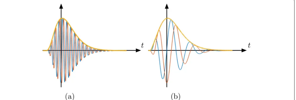
Waveletsψγ1(t)andψγ2(t)are designed as fourth-order Gammatone wavelets with one vanishing moment [35] and are shown in Fig. 1. In the context of auditory scene analysis, the asymmetric envelopes of Gammatone wavelets are more biologically plausible than the symmet-ric, Gaussian envelopes of the more widely used Mor-let waveMor-lets. Indeed, it allows to reproduce two impor-tant psychoacoustic effects in the mammalian cochlea: the asymmetry of temporal masking and the asymme-try of spectral masking [41]. The asymmetry of tem-poral masking is the fact that a masking noise has to be louder if placed after the onset of a stimulus rather than before. Likewise, because critical bands are skewed towards higher frequencies, a masking tone has to be

louder if it is above the stimulus in frequency rather than below. It should also be noted that Gammatone wavelets follow the typical amplitude profile of natural sounds, beginning with a relatively sharp attack and ending with a slower decay. As such, they are similar to filters discov-ered automatically by unsupervised encoding of natural sounds [30, 31]. In addition, Gammatone wavelets have proven to outperform Morlet wavelets on a benchmark of supervised musical instrument classification from scat-tering coefficients [20]. This suggests that, despite being hand-crafted and not learned, Gammatone wavelets pro-vide a sparser time-frequency representation of acoustic scenes compared to other variants. More information can be found in Additional file1.

4 Feature design

Before constructing models for similarity estimation, it is beneficial to process scattering coefficients to improve invariance, normality, and generalization power. In this section, we review two transformations which achieve these properties: logarithmic compression and standardisation.

4.1 Logarithmic compression

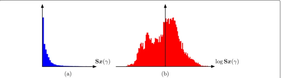
Many algorithms in pattern recognition, including near-est neighbor classifiers and support vector machines, tend to work best when all features follow a standard nor-mal distribution across all training instances [12]. Yet the distribution of the scattering coefficients is skewed towards larger values. We can reduce this skewness by applying a pointwise concave transformation to all coeffi-cients. In particular, we find that the logarithm performs particularly well in this respect. Figure2shows the distri-bution of an arbitrarily chosen scattering coefficient over the DCASE 2013 dataset, before and after logarithmic compression.

Taking the logarithm of a magnitude spectrum is ubiq-uitous in audio signal processing. Indeed, it is corrob-orated by the Weber-Fechner law in psychoacoustics,

which states that the sensation of loudness is roughly proportional to the logarithm of the acoustic pressure. We must also recall that the measured amplitude of sound sources often decays polynomially with the distance to the microphone—a source of spurious variability in scene classification. Logarithmic compression linearizes this dependency, facilitating the construction of powerful invariants at the classifier stage.

4.2 Standardization

LetSx(γ,n) be a dataset, whereγ andndenote feature and sample indices, respectively. Many algorithms operate better on features which have zero mean and unit variance to avoid mismatch in numeric ranges [12]. To standardize Sx(γ,n), we subtract the sample mean vector μ[Sx(γ )] fromSx(γ,n) and divide the result by the sample stan-dard deviation vector σ[Sx](γ ). The vectors μ[Sx(γ )] andσ[Sx](γ )are estimated from the entire dataset.

5 Acoustic scene similarity retrieval

As discussed in Section2, results in sound perception sug-gest the appropriateness of source-driven representations of auditory scenes for predicting high-level properties. While this can be addressed in the supervised case using late integration of discriminative classifiers [1], this is not directly feasible in the unsupervised case. As the detection of events is still an open problem [32], we consider in this paper a generic quantization scheme in order to identify and represent time intervals of the scene that are coherent, thus likely to be dominated by a given source of interest.

Given a set of d-dimensional feature vectors Xu =

xu₁,. . .,xu_L, extracted from the scene su, where u = {1, 2,. . .,U}, we would like to partition Xu into a set Cu =

cu₁,. . .,cu_M of M clusters. This partition is obtained by minimizing the variance of each cluster and known as ak-means clustering [18]. Each scene su is then described by a set of clustersCu. Note that this quantization approach differs from unsupervised learning schemes such as the ones studied in [5], where the scene

features are projected in a dictionary learned from the entire dataset. Here, with the aim of better balancing the influence of salient sound events and texture-like sounds on the final decision, the similarity between two scenes is computed based on the similarity of their centroids.

The similarity between the scene centroidsμu_mover the entire dataset is computed using a radial basis function (RBF) kernelKcombined with a local scaling method [39]:

K_mnuv =exp

− μum−μvn2

μu

m−μum,qμvn−μvn,q

. (6)

Here,μu_m,qandμv_n,qare theqthnearest neighbors to the centroidsμu_mandμv_n, respectively, and the double bars· denote the Euclidean norm.

To compute the similarity between two scenes, we con-sider several centroid-based similarity metrics:

• Relevance-based quantization closest similarity (RbQ-c): the similarity between two scenessuandsvis equal to the largest similarity between their centroids

max m,n K

uv

mn, (7)

• Relevance-based quantization average similarity (RbQ-a): the similarity between two scenessuandsv is equal to the average of their centroid similarities

1 M2

m,n

K_mnuv (8)

and,

• Relevance-based quantization weighted similarity (RbQ-w): the similarity between two scenes is computed using a variant of the earth mover’s distance applied to the set of centroids each weighted by the number of frames assigned to its cluster.

ForRbQ-w, each scene is represented by a signature

pu=μu₁,wu₁,μu₂,wu₂,. . .,μu_M,wu_M, (9)

where each of theMcentroidsμu₁,. . .,μu_Mare paired with corresponding weightswu₁,. . .,wu_M. The weightwu_mfor the mth centroidμu_mis the number of frames belonging to a particular cluster. The similarity between scenes is then given by a cross-bin histogram distance known as the non-normalized earth mover’s distance EMD introduced by [28]. TheEMD computes the distance between two his- tograms by finding the minimal cost for transforming one histogram into the other, where cost is measured by the number of transported histogram counts multiplied by a dissimilarity measure between the histogram bins. Here, that measure is given by 1−Kuv

mn.

6 Experiments

To evaluate the representations introduced in the previ-ous section, we apply it to the acprevi-oustic scene similarity

retrieval task. Results demonstrate the improved perfor-mance of the relevance-based quantization of scattering coefficients compared to baseline methods using sum-mary statistics of MFCCs. The implementations of the presented methods and the experimental protocol are available online.1

6.1 Dataset

The experiments in this paper are carried out on the pub-licly available DCASE 2013 dataset [32]. Although the dataset was constructed for the task of acoustic scene clas-sification, where the goal is to correctly assign the class of a given recording, we can use the same recordings and class labels for the task of acoustic scene similarity retrieval. The dataset consists of two parts, a public and a private subset, each made up of 100 acoustic scene record-ings sampled at 44100 Hz and 30 s in duration. The dataset is evenly divided into 10 acoustic scene classes:bus,busy street,office,open air market,park,quiet street,restaurant, supermarket,tube, andtube station. The recordings were made by three different recordists at a wide variety of loca-tions in the Greater London area over a period of several months. In order to avoid any correlation between record-ing conditions and label distribution, all recordrecord-ings were carried out under moderate weather conditions, at vary-ing times of day and week, and each recordist recorded each scene type. As a result, the dataset enjoys significant intra-class diversity while remaining of manageable size, making it suitable for evaluation of algorithmic design choices [15]. As an illustration, Fig. 3 represents the wavelet scalogram of one recording within the DCASE 2013, labeled aspark.

6.2 Feature design

We perform our experiments using both scattering coef-ficients and MFCCs. For the scattering transform, each 30-second scene is described by 128 vectors of dimen-sion 1367 computed with half-overlapping windowsφ(t) of durationT = 372 ms, for a total of 24 s. Here, we dis-card 3 s from the beginning and end of the scene to avoid boundary artifacts. We also conduct experiments with and without logarithmic compression of the scattering coefficients (see Section4.1).

MFCCs are computed for windows of 50 ms and hops of 25 ms with full frequency range. The standard config-uration of 39 coefficients coupled with an average-energy measure performs best in preliminary tests, so we use this in the following. We average the coefficients using 250 ms long non-overlapping windows so that each window rep-resents structures of scales close to that of scattering coefficients.

6.3 Evaluation and algorithm

Fig. 3Wavelet scalogramx1(t,γ1)of the audio recordingpark04in the DCASE 2013 dataset. We observe that this acoustic scene is a mixture of transient events (chirping birds, footsteps) and stationary texture (flowing water)

at rank k (p@k). This number is computed by taking a query item and counting the number of items of the same class within thek closest neighbors, and then averaging over all query items. We determine these neighbors using one of the proposed similarity measuresRbQ-c, RbQ-a, or RbQ-w. We compute p@k for k = {1,. . ., 9}, since each class only has 10 items. Note that p@1 is equal to the classification accuracy obtained by the nearest-neighbor classifier in a leave-one-out cross-validation setting.

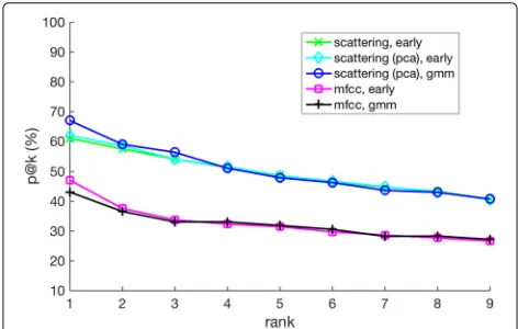
The RbQ measures are compared to commonly used early integration approachearly, which consists in aver-aging over time the feature set of each scene, resulting in one feature vector per scene. The distance on this aver-age feature vector is then used to determinep@k. For the BoF approach of Aucouturier et al. [3], GMMs are esti-mated for each scene using the expectation-maximization (EM) algorithm [8,24]. The similarity between a given pair of scene GMMs is then calculated through Monte Carlo sampling approximation. To ensure convergence of the EM algorithm for the scattering features, we reduce their dimension from 1367 to 30 by projecting the features onto the top 30 principal components of the dataset. The num-ber of Gaussians is optimized for each type of features by grid search in the range [ 2, 20]. Bestp@5 is reached with 8 and 4 Gaussians, respectively, for MFCCs and scattering features. Recommended number of Gaussians for MFCCs given in [3] is 10.

The scaling parameterqof the RBF kernels (see Eq.6) is set to 10% of the number of data points to cluster. As the number of Gaussians for the BoF approach, the number of clustersM controls the level of abstraction. For each method, unless otherwise stated, the parameterMis set to 8. It thus allows 8 different types of observations to be modeled, which seems reasonable given the duration of the scene (30 s). Note that this is the only free parameter in the proposed method. However, except forRbQ-a, the results are not very sensitive to the choice ofM, as long

as it is large enough to characterize the seen. A numerical demonstration is provided at the end of the next section.

7 Results

Results for the acoustic scene similarity retrieval task demonstrate that logarithmically compressed scattering features outperform MFCCs. Combining these with the RbQcluster model, improvements are obtained over tra-ditional BoF and summary statistic measures.

7.1 Baselines

As seen in Fig. 4, scattering features significantly out-perform the baseline MFCCs for both BoF and early integration schemes. This is expected, as the scattering transform extends the MFCCs by including supplemen-tary amplitude modulation information [1]. We also note that applying principal components analysis reduction to the scattering transform has little effect for the early inte-gration scheme. In the context of summary statistics, 30

dimensions are sufficient to discriminate between audi-tory scenes.

Comparing the BoF to early integration, both approaches perform similarly for MFCCs and PCA-reduced scattering features alike. This is in line with previous results on BoF [15], where it is found to perform similarly as similarity retrieval on features averaged over the entire recording.

The early approach being simpler in terms of implemen-tation and runtime complexity, we retain this method as baseline for the remainder of the experiments.

7.2 Logarithmic compression

Figure5shows that logarithmic compression of the scat-tering features is beneficial. For clarity’s sake, data is shown for the early approach only, but an equivalent gain is achieved for the relevance-based quantization approaches.

7.3 MFCC vs. scattering transform

Irrespective of the rank k considered, the best result is achieved for the scattering transform with logarithmic compression using the RbQ-c approach. Overall, log-compressed scattering coefficients systematically outper-form MFCCs (Fig. 6). This is to be expected since the scattering coefficients capture larger-scale modulations, as opposed to MFCCs which only describe the short-time spectral envelope.

7.4 Relevance-based quantization vs. early integration For the scattering transform, bothRbQ-candRbQ-w out-perform early, thus confirming the benefits of using a relevance-based quantization (RbQ) to improve the simi-larity measures between the scenes. However, it is worth noting that RbQ-a performs comparably to or worse thanearly, showing that the discriminant information is destroyed by averaging the contributions from all cen-troids. This result is in line with the findings of [15]. To

Fig. 5Acoustic scene similarity retrieval in the DCASE 2013 private dataset: precisions at rankk(p@k) obtained for scattering with or without logarithmic compression, as a function of the rankk

Fig. 6Acoustic scene similarity retrieval in the DCASE 2013 private dataset: precisions at rankk(p@k) obtained for MFCCs and scattering with logarithmic compression

take advantage of such a representation, we need to select certain representative centroids when comparing quan-tized objects. The same behavior is observed for MFCCs, with RbQ-c and RbQ-w outperforming early, which is equivalent to the state-of-the-art BoF model, as seen pre-viously.

Furthermore, it appears that RbQ-c is better able to characterise the classes compared to RbQ-w. Although not the only way of incorporating the number of frames associated to each centroid, the earth mover’s distance is a rather natural way of doing so. Its worse performance therefore suggests that including this information may not always be desirable. Indeed, nothing a priori indicates that the discriminant information between two scenes lies within the majority of their frames. On the contrary, two similar environments may share a lot of similar sound sources with only a few sources discriminating between them.

Withp@5 as our metric (cf. [3] and [15]), we see that replacing MFCCs by the logarithmically compressed scat-tering transform increases performance from 0.31 to 0.49. In addition, the relevance-based quantization using the closest similarity (RbQ-c) further improves the perfor-mance to 0.54 for a global increase of 0.23.

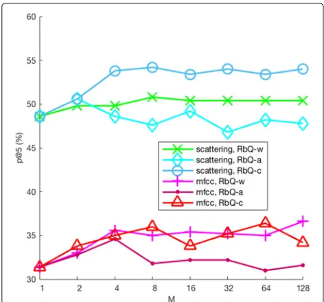
7.5 Sensitivity to number of clustersM

We now study the sensitivity of the precision at rank 5 (p@5) with respect to the number of clusters M. The results are shown in Fig.7.

Fig. 7Acoustic scene similarity retrieval in the DCASE 2013 private dataset: precision at rank 5 (p@5) obtained for different methods as a function of the number of clustersM

for better characterization of various signal structures in the scenes. As the number of clusters increases, the RbQ-amethod performs worse for both scattering features and MFCCs since any distinct objects are averaged out by clus-ters representing the background. TheRbQ-wandRbQ-c methods do better in this regard, as they are better able to emphasize the clusters that discriminate well between scenes.

UsingRbQ-c, therefore, we are not very sensitive to the choice of M, as long as it is large enough to allow for separation of the discriminative sound objects from the background. This motivates our choice ofM = 8 for the previous experiments in this section.

8 Conclusions

This paper presents a new approach for modeling acous-tic scenes based on scattering transforms at small scales and cluster-based representations at large scales. Com-pared to traditional BoF and summary statistics models, this representation allows for the characterization of dis-tinct sound events superimposed on a stationary texture, a concept which has strong grounding in the cognitive psychology literature. To adequately capture such dis-tinct events, we develop a cluster-based model and val-idate it using experiments on acoustic scene similarity retrieval. For this task, we show significant improvements over the traditional BoF and summary statistics models based on both standard MFCCs and scattering features. These outcomes shall be studied further in future work by considering larger databases and emerging tasks in ecoacoustics [34,38].

Endnote

1_{https://github.com/mathieulagrange/}

paperRelevanceBasedSimilarity

Additional file

Additional file 1:Supplementary material. (PDF 63 KB)

Funding

This study is co-funded by the ANR under project referenc ANR-16-CE22-0012.

Availability of data and materials

The dataset supporting the conclusions of this article is available in the dcase2013 repository,http://c4dm.eecs.qmul.ac.uk/sceneseventschallenge/ description.html. The software supporting the conclusions of this article is available in:

• Companion website:https://github.com/mathieulagrange/ paperRelevanceBasedSimilarity

• Programming language: MATLAB • License: GNU GPL

• Any restrictions to use by non-academics: license needed

Authors’ contributions

GL and VL carried out the numerical experiments and drafted the manuscript. VL, GL, JA, and ML participated in the design of the study and helped to draft the manuscript. All authors read and approved the final manuscript.

Competing interests

The authors declare that they have no competing interests.

Publisher’s Note

Springer Nature remains neutral with regard to jurisdictional claims in published maps and institutional affiliations.

Author details

1_{LS2N, CNRS, Ecole Centrale de Nantes, France.}2_{Center for Computational} Biology, Flatiron Institute, New York, NY, USA.3New York University, New York, NY, USA.

Received: 23 February 2018 Accepted: 26 August 2018

References

1. J. Andén, S. Mallat, Deep scattering spectrum. IEEE Trans. Sig. Process.

62(16), 4114–4128 (2014)

2. R. Arandjelovic, A. Zisserman, inIEEE International Conference on Computer Vision (ICCV). Look, listen and learn (IEEE, 2017), pp. 609–617

3. J. J. Aucouturier, B. Defreville, F. Pachet, The bag-of-frames approach to audio pattern recognition: A sufficient model for urban soundscapes but not for polyphonic music. J. Acoust. Soc. Am.122(2), 881–891 (2007) 4. Y. Aytar, C. Vondrick, A. Torralba, inAdvances in Neural Information

Processing Systems. Soundnet: Learning sound representations from unlabeled video (Curran Associates, Inc., Red Hook, 2016), pp. 892–900 5. V. Bisot, R. Serizel, S. Essid, G. Richard, in2016 IEEE International Conference

on Acoustics, Speech and Signal Processing (ICASSP). Acoustic scene classification with matrix factorization for unsupervised feature learning (IEEE, New York, 2016), pp. 6445–6449

6. V. Chudáˇcek, J. Anden, S. Mallat, P. Abry, M. Doret, Scattering transform for intrapartum fetal heart rate variability fractal analysis: A case study. IEEE Trans. Biomed. Eng.61(4), 1100–1108 (2013)

7. S. Davis, P. Mermelstein, Comparison of parametric representations for monosyllabic word recognition in continuously spoken sentences. IEEE Trans. Acoust. Speech Sig. Process.28(4), 357–366 (1980)

8. A. P. Dempster, N. M. Laird, D. B. Rubin, Maximum likelihood from incomplete data via the EM algorithm. J. Royal Stat. Soc. B Stat. Methol.

9. D. Dubois, C. Guastavino, M. Raimbault, A cognitive approach to urban soundscapes: Using verbal data to access everyday life auditory categories. Acta Acustica U. Acustica.92(6), 865–874 (2006)

10. J. R. Gloaguen, A. Can, M. Lagrange, J. F. Petiot, inWorkshop on Detection and Classification of Acoustic Scenes and Events. Estimating traffic noise levels using acoustic monitoring: A preliminary study, (2016) 11. F. Guyot, S. Nathanail, F. Montignies, B. Masson, inProceedings Forum

Acusticum. Urban sound environment quality through a physical and perceptive classification of sound sources: A cross-cultural study, (Budapest, Hungary, 2005)

12. C. W. Hsu, C. C. Chang, C. J. Lin, et al.,A practical guide to support vector classification. Tech. rep.(National Taiwan University, Taipei, 2003) 13. J. Kang,Urban sound environment. (CRC Press, 2006)

14. S. Kuwano, S. Namba, T. Kato, J. Hellbrck, Memory of the loudness of sounds in relation to overall impression. Acoust. Sci. Technics.4(24) (2003). The Acoustical Society of Japan

15. M. Lagrange, G. Lafay, B. Defreville, J. J. Aucouturier, The bag-of-frames approach: A not so sufficient model for urban soundscapes. JASA Express Lett.138(5), 487–492 (2015)

16. C. Lavandier, B. Defréville, The contribution of sound source

characteristics in the assessment of urban soundscapes. Acta Acustica U. Acustica.92(6), 912–921 (2006). Stuttgart, Germany

17. H. Lee, P. Pham, Y. Largman, A. Ng, inProc. NIPS. Unsupervised feature learning for audio classification using convolutional deep belief networks, (2009), pp. 1096–1104

18. S. Lloyd, Least squares quantization in PCM. IEEE Trans. Inf. Theory.28(2), 129–137 (1982)

19. B. Logan, inProceedings of the International Symposium on Music Information Retrieval. Mel frequency cepstral coefficients for music modeling, (2000)

20. V. Lostanlen,Convolutional operators in the time-frequency domain. Ph.D. thesis. (École Normale Supérieure, Paris, 2017)

21. V. Lostanlen, C. E. Cella, inProceedings of the International Society for Music Information Retrieval Conference. ISMIR. Deep convolutional networks in the pitch spiral for music instrument classification, (2016)

22. S. Mallat, Group Invariant Scattering. Commun. Pur. Appl. Math.65(10), 1331–1398 (2012). Wiley, New York

23. J. H. McDermott, M. Schemitsch, E. P. Simoncelli, Summary statistics in auditory perception. Nat. Neurosci.16(4), 493–498 (2013)

24. T. K. Moon, The expectation-maximization algorithm. IEEE Signal Proc. Mag.13(6), 47–60 (1996). New York

25. I. Nelken, Processing of complex stimuli and natural scenes in the auditory cortex. Curr. Opin. Neurobiol.14(4), 474–480 (2004). Elsevier, Amsterdam 26. I. Nelken, A. de Cheveigné, An ear for statistics. Nat. Neurosci.16(4),

381–382 (2013)

27. S. R. Ness, H. Symonds, P. Spong, G. Tzanetakis, The Orchive: Data mining a massive bioacoustic archive. Int. Work. Mach. Learn. Bioacoustics (2013) 28. O. Pele, M. Werman, inEuropean Conference on Computer Vision. A linear

time histogram metric for improved SIFT matching (Springer, 2008), pp. 495–508

29. P. Ricciardi, P. Delaitre, C. Lavandier, F. Torchia, P. Aumond, Sound quality indicators for urban places in Paris cross-validated by Milan data. J. Acoust. Soc. Am.138(4), 2337–2348 (2015)

30. T. Sainath, R. J. Weiss, A. Senior, K. W. Wilson, O. Vinyals, inProceedings of INTERSPEECH. Learning the speech front-end with raw waveform cldnns, (2015)

31. E. C. Smith, M. S. Lewicki, Efficient auditory coding. Nature.439(7079), 978–982 (2006)

32. D. Stowell, D. Giannoulis, E. Benetos, M. Lagrange, M. D. Plumbley, Detection and classification of acoustic scenes and events. IEEE Trans. Multimed.17(10), 1733–1746 (2015)

33. D. Stowell, M. D. Plumbley, Large-scale analysis of frequency modulation in birdsong databases. Methods Ecol. Evol.11(2013). New York 34. J. Sueur, A. Farina, Ecoacoustics: the ecological investigation and

interpretation of environmental sound. Biosemiotics.8(3), 493–502 (2015). Berlin

35. A. Venkitaraman, A. Adiga, C. S. Seelamantula, Auditory-motivated Gammatone wavelet transform. Sig. Process.94, 608–619 (2014) 36. I. Waldspurger, inProc. SampTA. Exponential decay of scattering

coefficients (IEEE, New York, 2017), pp. 143–146. Conference was held in Tallinn, Estonia

37. P. S. Warren, M. Katti, M. Ermann, A. Brazel, Urban bioacoustics: It’s not just noise. Anim. Behav.71(3), 491–502 (2006)

38. J. Wimmer, M. Towsey, P. Roe, I. Williamson, Sampling environmental acoustic recordings to determine bird species richness. Ecol. Appl.23(6), 1419–1428 (2013)

39. L. Zelnik-Manor, P. Perona, inAdvances in Neural Information Processing Systems. (NIPS) No. 17. Self-tuning spectral clustering (MIT Press, Cambridge, 2004), pp. 1601–1608

40. L. Zhang, M. Towsey, J. Zhang, P. Roe, Classifying and ranking audio clips to support bird species richness surveys. Ecol. Inform.34, 108–116 (2016) 41. E. Zwicker, H. Fastl,Psychoacoustics: Facts and models, vol. 22. (Springer