R E S E A R C H
Open Access
New results on anti-periodic boundary value
problems for second-order nonlinear
differential equations
Ruixi Liang
**Correspondence:
[email protected] School of Mathematical Sciences and Computing Technology, Central South University, Changsha, Hunan 410075, China
Abstract
This paper is concerned with the solvability of anti-periodic boundary value problems for second-order nonlinear differential equations. By using topological methods, some sufficient conditions for the existence of solution are obtained, which extend and improve the previous results.
MSC: 34B05
Keywords: anti-periodic boundary value problem; existence of solution; nonlinear
1 Introduction
In this paper, we will consider the existence of solutions to second-order differential equa-tions of the type
x(t) =ft,x(t),x(t), t∈J= [,T], (.) subject to the anti-periodic boundary conditions
x() +x(T) = , x() +x(T) = , (.)
whereT is a positive constant andf : [,T]×R×R→Ris continuous. Equation (.) subject to (.) is called an anti-periodic boundary value problem.
Anti-periodic problems have been studied extensively in recent years. For example, anti-periodic boundary value problems for ordinary differential equations were considered in [–]. Also, anti-periodic boundary conditions for impulsive differential equations, partial differential equations and abstract differential equations were investigated in [–]. The methods and techniques employed in these papers involve the use of the Leray-Schauder degree theory [, ], the upper and lower solutions [, –], and a fixed point theorem []. By using Schauder’s fixed point theorem and lower and upper solutions method, Wang and Shen in [] considered the anti-periodic boundary value problem (.) and (.) when a first-order derivative is not involved explicitly in the nonlinear termf, namely equation (.) reduces to
x(t) =ft,x(t), t∈J. (.)
They proved the following theorems.
Theorem .([, Theorem .]) Assume there exist constants <r< ,l> ,and func-tions p,q,h∈C(J,R)such that
uf(t,u)≤p(t)u+q(t)|u|r+h(t) (.)
for t∈J and|u|>l.Further suppose that
T
p+(s)ds< ,
where p+(t) =max{p(t), }.Then(.)and(.)have at least one solution.
Theorem .([, Theorem .]) Letγbe a positive constant.Assume there exist a
continu-ous and nondecreasing functionψ: [,∞)→(,∞)and a nonnegative function p∈C(J,R)
with
f(t,u) +γu≤p(t)ψ|u|
for t∈J and u∈R.Further suppose that
lim sup u→∞
ψ(u)
u <K:=
γ(eγT+ )
eγT(eγT– )T
p(s)ds
. (.)
Then(.)and(.)have at least one solution.
In this paper, we are interested in the existence of a solution to the anti-periodic bound-ary value problem (.) and (.). The significant point here is that the right-hand side of (.) may depend onx. The dependence of right-hand side onxis naturally seen in many physical phenomena, and we refer the readers to [, ] for some nice examples. If there appearsxin nonlinear term, the relative boundary value problem will be more complicated. Meanwhile, we note equation (.) or (.) implies thatf(t,x) is at most lin-ear forx, so the problem has not been solved whenf(t,x) is super-linear forx. Motivated by the above two aspects, we devote ourselves to studying the anti-periodic boundary value problem (.) and (.).
The paper is organized as follows. In Section , we reformulate the anti-periodic bound-ary value problem (.) and (.) as an equivalent integral equation, which is a widely used technique in the theory of boundary value problem. In Section , a general existence result is presented for (.) and (.). The result provides a natural motivation for the obtention ofa prioribounds on solutions and greatly minimizes the proofs of the new results in the following section. The main tool used here is the Leray-Schauder topological degree. In Section , some new conditions are presented for (.) and (.). The new conditions involve linear or quadratic growth constraints on|f(t,p,q)|in|q|.
2 Preliminaries
If a functionx∈C(J,R) satisfies equations (.) and (.), we callxa solution of (.) and
(.). LetC(J,R) be a Banach space with the normx=max{|x|,|x|}, where|x|=
Letλ> ,δ(t)∈C(J,R) and consider the anti-periodic boundary value problem ⎧
⎨ ⎩
x(t) –λx(t) =δ(t), t∈J,
x() +x(T) = , x() +x(T) = .
(.)
Lemma . x is a solution of(.)if and only if x satisfies
x(t) = T
G(t,s)δ(s)ds, (.)
where
G(t,s) = ⎧ ⎨ ⎩
eλ(t–s)–eλ(T–t+s)
λ(+eλT) , ≤s<t≤T, eλ(s–t)–eλ(T+t–s)
λ(+eλT) , ≤t≤s≤T.
Proof Supposex(t) is a solution of (.) and denoteD=dtd, then the first equation of (.) can be rewritten as
(D–λ)(D+λ)x(t) =δ(t). (.)
Let
y(t) = (D+λ)x(t), (.)
then from (.), we have
(D–λ)y(t) =δ(t).
Multiplying both sides of the above equation bye–λt and integrating from totyields
e–λty(t) –y() = t
δ(s)e–λsds,
y(t) =eλt
y() + t
δ(s)e–λsds
, t∈J,
wherey() =x() +λx().
Similarly, multiplying the two sides of (.) byeλtand integrating from totyields
x(t) =e–λt
x() + t
eλsy(s)ds
. (.)
By direct computation, we get
t
eλsy(s)ds
= λ
y()eλt– +
t
eλt–eλsδ(s)e–λsds
Substituting (.) into (.),
x(t) = λ
x() +λx()eλt+λx() –x()e–λt
– t
e–λ(t–s)–eλ(t–s)δ(s)ds
. (.)
Hence,
x() = λ
x() +λx()+λx() –x(),
x(T) = λ
x() +λx()eλT+λx() –x()e–λT–
T
e–λ(T–s)–eλ(T–s)δ(s)ds
.
Further from (.),
x(t) = λ
x() +λx()λeλt+λx() –x()(–λ)e–λt
– t
–λe–λ(t–s)–λeλ(t–s)δ(s)ds
,
and therefore
x() = λ
x() +λx()λ+λx() –x()(–λ),
x(T) = λ
x() +λx()λeλT–λx() –x()λe–λT
– T
–λe–λ(T–s)–λeλ(T–s)δ(s)ds
.
Taking into accountx() +x(T) = ,x() +x(T) = , we obtain
x() +λx() = –
eλT+
T
eλ(T–s)δ(s)ds, (.)
and
λx() –x() =
e–λT+
T
e–λ(T–s)δ(s)ds. (.)
Substituting (.) and (.) into (.), we get
x(t) = λ
–
eλT+
T
eλ(T–s)δ(s)ds·eλt+
e–λT+
T
e–λ(T–s)δ(s)ds·e–λt
– t
e–λ(t–s)–eλ(t–s)δ(s)ds
= λ
+eλT
–
T
eλ(T+t–s)δ(s)ds+ +eλT t
eλ(t–s)δ(s)ds
+
+e–λT
T
e–λ(T+t–s)δ(s)ds– +e–λT t
e–λ(t–s)δ(s)ds
= λ
+eλT
t
eλ(t–s)δ(s)ds– T
t
eλ(T+t–s)δ(s)ds
+
+e–λT
–
t
e–λ(t–s)δ(s)ds+ T
t
e–λ(T+t–s)δ(s)ds
= λ
t
eλ(t–s)
+eλT ·δ(s)ds–
t
e–λ(t–s)
+e–λT ·δ(s)ds
+ T
t
e–λ(T+t–s)
+e–λT ·δ(s)ds–
T
t
eλ(T+t–s)
+eλT ·δ(s)ds
=
λ( +eλT)
t
eλ(t–s)–eλ(T–t+s)δ(s)ds+
T
t
eλ(s–t)–eλ(T+t–s)δ(s)ds
= T
G(t,s)δ(s)ds.
That is,x(t) is a solution of (.).
On the other hand, assumex(t) is a solution of (.). Then
x(t) = T
∂G(t,s)
∂t δ(s)ds=
T
G*(t,s)δ(s)ds,
where
G*(t,s) = (eλT+ )
⎧ ⎨ ⎩
eλ(t–s)+eλ(T–t+s), ≤s<t≤T,
–eλ(s–t)–eλ(T+t–s), ≤t≤s≤T.
And
x(t) = t
[λeλ(t–s)–λeλ(T–t+s)]
(eλT+ ) δ(s)ds+
[ +eλT]
(eλT+ )δ(t)
+ T
t
[λeλ(s–t)–λeλ(T+t–s)]
(eλT+ ) δ(s)ds–
[– –eλT]
(eλT+ )δ(t)
=λ T
G(t,s)δ(s)ds+δ(t)
=λx(t) +δ(t).
Direct computation yields
x() +x(T) = , x() +x(T) = .
Hence,x(t) is a solution of (.). This proof is complete.
For later use, we present the following estimations:
max
(t,s)∈J×JG(t,s)=
eλT–
λ( +eλT), (tmax,s)∈J×JG
*(t,s)=
. (.)
Combining Lemma . and equation (.), we can easily get
Theorem . The anti-periodic boundary value problem(.)and(.)is equivalent to the following integral equation:
x(t) = T
G(t,s)fs,x(s),x(s)–λx(s)ds, (.)
whereλ> and G(t,s)is defined in Lemma..
Define an operatorT:C(J,R)→C(J,R) by
Tx(t) := T
G(t,s)fs,x(s),x(s)–λx(s)ds. (.)
Lemma . T:C(J,R)→C(J,R)is completely continuous.
Proof Noting the continuity off, this follows in a standard step-by-step process and so is
omitted.
In view of Theorem ., we obtain
Theorem . x∈C(J,R)is a solution of the anti-periodic boundary value problem(.)
and(.)if and only if x∈C(J,R)is the fixed point of the operator T.
3 General existence
In this section, an abstract existence result is presented for (.) and (.). The obtained result emphasizes the natural search fora prioribounds on solutions to the boundary value problem, which will be conducted in the following section.
Firstly, we introduce some basic properties of the Leray-Schauder degree. For more de-tail, we refer an interested reader to [, ].
Theorem . The Leray-Schauder degree has the following properties.
(i) (Homotopy invariance)Let⊂X×[, ]be a bounded open set,and letF:¯ →X
be compact.Ifx–F(x,t)=zfor each(x,t)∈∂,thendLS(I–F(·,t),t,z)is
independent oft.
(ii) (Existence)IfdLS(I–f,,z)= ,thenz∈(I–f)().
Now, we give the main result of this section.
Theorem . Let M,N andλbe positive constants in R and f : [,T]×R×R→R be continuous.Consider the family of anti-periodic boundary value problems:
⎧ ⎨ ⎩
x(t) –λx(t) =μ[f(t,x(t),x(t)) –λx(t)], t∈J,μ∈[, ],
x() +x(T) = , x() +x(T) = . (.)
If all potential solutions to(.)satisfy
with M and N independent ofμ,then the anti-periodic boundary value problem(.)and
(.)has at least one solution.
Proof In view of Theorem ., we want to show there exists at least onex∈C(J,R) with
xsatisfyingTx=x. This solution will then naturally be inC(J,R).
Consider the family of problems associated with (.), namely
H(x,μ) :=x–μTx= , μ∈[, ]. (.)
Note that (.) is equivalent to the family of anti-periodic boundary value problems (.). Now, let⊂C(J,R) with
:=x∈C(J,R) :|x|<M,x<N
.
From Lemma ., we know thatT:→C(J,R) is completely continuous. Therefore,H: ×[, ]→C(J,R) is a compact mapping. By the assumption of the theorem, all possible solutionsx∈must satisfyx∈, and thus
H(x,μ)= , ∀x∈∂andμ∈[, ].
Hence, the following Leray-Schauder degrees are defined and the homotopy invariance principle in Theorem . applies:
dLSH(x,μ),, =dLSH(x, ),, =dLSH(x, ),, = ,
since ∈. By the existence property of the Leray-Schauder degree, (.) has at least one solution infor allμ∈[, ]. And hence (.) and (.) has at least one solution.
4 Main results
In this section, some existence theorems are presented.
Theorem . Letα,βand Kbe nonnegative constants andλ> .If f is continuous and
satisfies
f(t,p,q) –λp≤α|p|+β|q|+K, (t,p,q)∈J×R×R,
with
λeλT+ –β
eλT– > ,
and
eλT+ eλT– λ
–λβ
–α> ,
Proof Consider the family (.). We want to show the conditions of Theorem . hold for some positive constantsMandN.
Letx(t) be a solution to (.) and consider the equivalent equation (.), that is,
x(t) =μ T
G(t,s)fs,x(s),x(s)–λx(s)ds. (.)
For eacht∈[,T], we have x(t)=μ
T
G(t,s)fs,x(s),x(s)–λx(s)ds
≤
T
G(t,s)·fs,x(s),x(s)–λx(s)ds
≤
T
G(t,s)αx(s)+βx(s)+K
ds.
Since T
G(t,s)ds= t
G(t,s)ds+ T
t
G(t,s)ds
= t
|eλ(t–s)–eλ(T–t+s)|
λ( +eλT) ds+
T
t
|eλ(s–t)–eλ(T+t–s)|
λ( +eλT) ds
≤
t
eλ(t–s)+eλ(T–t+s)
λ( +eλT) ds+
T
t
eλ(s–t)+eλ(T+t–s)
λ( +eλT) ds
= –e
λ(t–s)+eλ(T–t+s)
λ( +eλT)
t
+e
λ(s–t)–eλ(T+t–s)
λ( +eλT)
T
t
= e λT–
λ(eλT+ ),
it follows that
|x|≤
eλT–
λ(eλT+ )
α|x|+βx+K
. (.)
Differentiating both sides of (.), we get
x(t) =μ T
G*(t,s)fs,x(s),x(s)–λx(s)ds,
then
x(t)≤ T
G*(t,s)α|x|+βx+K
ds,
and because of T
G*(t,s)ds= t
G*(t,s)ds+ T
t
G*(t,s)ds
= t
|eλ(t–s)+eλ(T–t+s)|
( +eλT) ds+
T
t
|eλ(s–t)+eλ(T+t–s)|
= t
eλ(t–s)+eλ(T–t+s)
( +eλT) ds+
T
t
eλ(s–t)+eλ(T+t–s)
( +eλT) ds
=–e
λ(t–s)+eλ(T–t+s)
λ( +eλT)
t
+e
λ(s–t)–eλ(T+t–s)
λ( +eλT)
T
t
= e λT–
λ(eλT+ ).
Therefore,
x≤ e
λT–
λ(eλT+ )
α|x|+βx+K
.
The rearrangement yields
x≤ (e
λT– )(α
|x|+K)
λ(eλT+ ) –β
(eλT– )
. (.)
By substituting (.) into (.) and rearranging, we obtain
|x|≤
K
eλT+
eλT–λ–λβ–α
:=M.
So,
x≤ (e
λT– )(α
M+K)
λ(eλT+ ) –β
(eλT– )
:=N.
Hence, Theorem . holds for positive constantsM=M+ andN=N+ . The solvability
of (.) and (.) now follows.
Theorem . Assume there exist nonnegative constantsα,Kandλ> such that
f(t,p,q) –λp<α
pf(t,p,q) +q+K, for(t,p,q)∈J×R×R,
then the anti-periodic boundary value problem(.)and(.)has at least one solution.
Proof Supposex(t) is a solution of (.), and in view of (.), we have
|x|=max
t∈J
μ
T
G(t,s)fs,x(s),x(s)–λx(s)ds
≤μmax t∈J
T
G(t,s)·fs,x(s),x(s)–λx(s)ds
≤max t∈J
T
G(t,s)μα
x(s)fs,x(s),x(s)+x(s)+μK
ds
≤
T
max
t∈J G(t,s)α
x(s)μfs,x(s),x(s)
+λ( –μ)x(s)+x(s)+K
≤ eλT–
λ( +eλT)
T
α
x(s)x(s) +x(s)+K
ds
= e λT–
λ( +eλT)
T α d ds
x(s)x(s)+K
ds
= e λT–
λ( +eλT)
α
x(T)x(T) –x()x()+KT
≤ eλT–
λ( +eλT)KT:=M.
Similarly,
x =μmax t∈J
T
G*(t,s)fs,x(s),x(s)–λx(s)ds
≤max t∈J
T
G*(t,s)αμ
x(s)fs,x(s),x(s)+x(s)+K
ds ≤ T max t∈J G
*(t,s)α
x(s)μfs,x(s),x(s)
+λ( –μ)x(s)+x(s)+K
ds ≤ T α
x(s)x(s) +x(s)+K
ds ≤ T α
x(s)x(s) +x(s)+K
ds
= α
x(T)x(T) –x()x()+ KT.
=
KT:=N.
Therefore, Theorem . holds for positive constantsM=M+ andN=N+ . The
solvability of (.) and (.) now follows.
Example . Consider the anti-periodic boundary value problem
⎧ ⎨ ⎩
x(t) =x(t) +x(t)(x(t))+sint, t∈[, ],
x() = –x(), x() = –x(). (.)
We claim (.) has at least one solution.
Proof LetT = , andf(t,p,q) =p+pq+sintin Theorem .. Chooseλ= , we get for
(t,p,q)∈[, ]×Rthat
f(t,p,q) –p=pq+sint≤ |p|q+sint,
and
Noteminv≥{v–v}> –, we havepq+q–|p|q=q(p–|p|+ ) > . Thus, forα= ,
K=
f(t,p,q) –p≤ |p|q+sint≤ |p|q+
≤q+pq+
≤q+pq+p–|p|+
≤α
pf(t,p,q) +q+K.
Then the conclusion follows from Theorem ..
Now, we reconsider the problem (.) and (.). The following result is obtained.
Theorem . Suppose f: [,T]×R→R is continuous.If there exist nonnegative constants
α,Kandλ> such that
|f(t,p) –λp|<αpf(t,p) +K, for(t,p)∈[,T]×R,
then(.)and(.)has at least one solution.
Proof The proof is similar to Theorem . and here we omit it.
An example to highlight the Theorem . is presented.
Example . Consider the anti-periodic boundary value problem given by ⎧
⎨ ⎩
x(t) =x+x+t, t∈[, ],
x() +x() = , x() +x() = . (.)
We claim (.) has at least one solution.
Proof Letf(t,p) =p+p+tand see that|f(t,p) –p| ≤ |p|+ for (t,p)∈[, ]×R. For α,Kandλto be chosen below, see that
αpf(t,p) +K
=α
p+p+pt+K
=p+ +p+pt+ for the choicesα= ,K=
=p+ +(p+t/)+ –t/
≥p+ for the chooseλ=
≥f(t,p) –p for all (t,p)∈[, ]×R.
Thus, the conditions of Theorem . hold and the solvability follows.
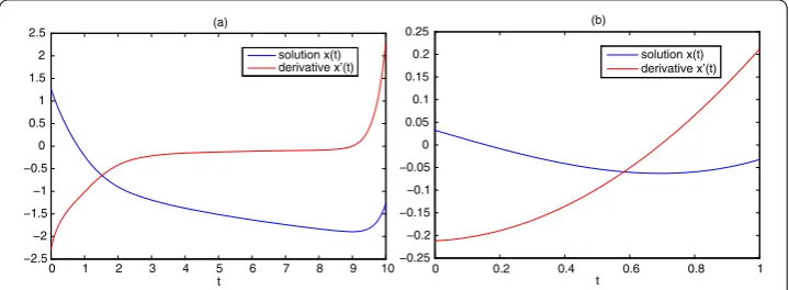
Figure 1 Solutions found by numerical stimulations with (a):f(t,p) =p3+p+t,T= 10 in equation
(4.5); (b):f(t,p,q) =p+pq2+ sint,T= 1 in equation (4.4).
Finally, in order to illustrate our main results, we use the ‘bvpc’ package in MATLAB to simulate. As shown in Figure (a) and (b), numerical simulations also suggest that Ex-amples . and . with the given coefficients admit at least one solution.
Competing interests
The author declares that they have no competing interests.
Author’s contributions
The author typed, read and approved the final manuscript.
Acknowledgements
The author would like to thank anonymous referees very much for helpful comments and suggestions which led to the improvement of presentation and quality of work. This research was partially supported by the NNSF of China (No. 11001274) and the Postdoctoral Science Foundation of Central South University and China (No. 2011M501280).
Received: 27 March 2012 Accepted: 27 September 2012 Published: 11 October 2012 References
1. Wang, KZ: A new existence result for nonlinear first-order anti-periodic boundary value problems. Appl. Math. Lett.
21, 1149-1154 (2008)
2. Franco, D, Nieto, JJ, O’Regan, D: Anti-periodic boundary value problem for nonlinear first order ordinary differential equations. Math. Inequal. Appl.6, 477-485 (2003)
3. Wang, WB, Shen, JH: Existence of solution for anti-periodic boundary value problems. Nonlinear Anal.70, 598-605 (2008)
4. Jankowski, T: Ordinary differential equations with anti-periodic and nonlinear boundary value conditions of anti-periodic type. Comput. Math. Appl.47, 1429-1436 (2004)
5. Yin, Y: Monotone iterative technique and quasilinearization for some anti-periodic problem. Nonlinear World3, 253-266 (1996)
6. Aftabizadeh, AR, Aizicovici, S, Pavel, NH: On a class of second-order anti-periodic boundary value problems. J. Math. Anal. Appl.171, 301-320 (1992)
7. Aftabizadeh, AR, Huang, Y, Pavel, N: Nonlinear third-order differential equations with anti-periodic boundary conditions and some optimal control problems. J. Math. Anal. Appl.192, 266-293 (1995)
8. Aftabizadeh, AR, Pavel, N, Huang, Y: Anti-periodic oscillations of some second-order differential equations and optimal control problems. J. Comput. Appl. Math.52, 3-21 (1994) (Oscillations in nonlinear systems: applications and numerical aspects)
9. Yin, Y: Remarks on first order differential equations with anti-periodic and nonlinear boundary value conditions. Nonlinear Times Dig.2, 83-94 (1995)
10. Ding, W, Xing, YP, Han, MA: Anti-periodic boundary value problems for first order impulsive functional differential equations. Appl. Math. Comput.186, 45-53 (2007)
11. Ahmad, B, Nieto, JJ: Existence and approximation of solutions for a class of nonlinear impulsive functional differential equations with anti-periodic boundary conditions. Nonlinear Anal.69, 3291-3298 (2008)
12. Luo, ZG, Shen, JH, Nieto, JJ: Anti-periodic boundary value problem for first-order impulsive ordinary differential equation. Comput. Math. Appl.49, 253-261 (2005)
13. Nakao, M: Existence of an anti-periodic solution for the quasilinear wave equation with viscosity. J. Math. Anal. Appl.
204, 754-764 (1996)
14. Souplet, P: Optimal uniqueness condition for the antiperiodic solutions of some nonlinear parabolic equations. Nonlinear Anal.32, 279-286 (1998)
16. Okochi, H: On the existence of anti-periodic solutions to nonlinear evolution equations associated with odd subdifferential operators. J. Funct. Anal.91, 246-258 (1990)
17. Pennline, JA: Constructive existence and uniqueness for two-point boundary value problems with a linear gradient term. Appl. Math. Comput.15(3), 233-260 (1984)
18. Granas, A, Guenther, R, Lee, J: Nonlinear Boundary Value Problems for Ordinary Differential Equations. Dissertationes Math. (Rozprawy Mat.), vol. 244 (1985)
19. Guo, DJ, Sun, JX, Liu, ZL: Functional Method of Nonlinear Ordinary Differential Equations. Shandong Science and Technology Press, Jinan (1995) (in Chinese)
20. Deimling, K: Nonlinear Functional Analysis. Springer, Berlin (1985)
doi:10.1186/1687-2770-2012-112