Euler’s line for enzyme kinetics

(1)

(ISSN: 2582-158X)

Vol. 01, Issue 09, pp.532-542, December, 2019 Available online at http://www.journalijrar.com

RESEARCH ARTICLE

EULER’S LINE FOR ENZYME KINETICS

1,

**_{*Vitthalrao Bhimasha Khyade,}**

2

_{Avram Hershko and}

3

_{Seema Karna Dongare}

1_{Department of Zoology, Shardabai Pawar Mahila Mahavidyalaya, Shardanagar Tal., Baramati Dist., Pune – 413115, India} 2_{Unit of Biochemistry, The B. Rappaport Faculty of Medicine, and the Rappaport Institute for Research in the Medical}

Sciences, Technion-Israel Institute of Technology, Haifa 31096, Israel

3_{P.G. Student, Department of Microbiology, Maharashtra Education Society's, Abasaheb Garware College,}

Karve Road, Pune – 411004, India

ARTICLE INFO ABSTRACT

A graph of the double-reciprocal equation is also called a Line weaver-Burk, reciprocal of velocity of enzyme reaction (1÷v) against reciprocal of substrate concentration [1÷S]. Lineweaver-Burk graphs are particularly useful for analyzing the changes in enzyme kinetics in the presence of inhibitors, competitive, non-competitive, or a mixture of the two. One more attempt is carried out for establishment of Euler’s line through the use of Line weaver-Burk plot. Line weaver-Burk plot (double reciprocal plot) is with positive value of (Km÷Vmax) as a slope. Euler Line for Enzyme Kinetics is with negative value of (Km÷Vmax) as a slope. The intercept on y-axis for Line weaver-Burk plot (double reciprocal plot) for Enzyme Kinetics correspond to: (1 ÷ Vmax). The intercept on y-axis for Euler Line for Enzyme Kinetics correspond to: [(Km +2) ÷ Vmax)]. Lineweaver-Burk plot (double reciprocal plot) and Euler Line for Enzyme Kinetics are intersecting at the point, x – co-ordinate of which correspond to: (1÷2) and y- co-ordinate of which correspond to: [(Km+2) ÷ Vmax]. The centroid for enzyme kinetics is always located between the orthocenter and the circumcenter of enzyme kinetics. The distance from the centroid to the orthocenter is always twice the distance from the centroid to the circumcenter of enzyme kinetics. Attempt may open a new avenue for three dimensional enzyme structure of and mechanism of enzyme involved reactions.

Key Words: Centroid, Orthocenter, Circumcenter, Euler’s line.

Copyright © 2019, Vitthalrao Bhimasha Khyade. This is an open access article distributed under the Creative Commons Attribution License, which permits unrestricted use, distribution, and reproduction in any medium, provided the original work is properly cited.

INTRODUCTION

Enzymes are protein molecules that manipulate other molecules the enzymes' substrates. These target molecules bind to an enzyme's active site and are transformed into products through a series of steps known as the enzymatic mechanism. Enzyme kinetics is the study of the chemical reactions that are catalyzed by enzymes. In enzyme kinetics, the reaction rate is measured and the effects of varying the conditions of the reaction are investigated. Studying an enzyme's kinetics in this way can reveal the catalytic mechanism of this enzyme, its role in metabolism, how its activity is controlled, and how a drug or an agonist might inhibit the enzyme (Kraut, Carroll and Herschlag (2003). The Michaelis-Menten equation arises from the general equation for an enzymatic reaction:

E + S ↔ ES ↔ E + P,

Where E is the enzyme, S is the substrate,

ES is the enzyme-substrate complex, and P is the product.

Thus, the enzyme combines with the substrate in order to form the ES complex, which in turn converts to product while preserving the enzyme.

The rate of the forward reaction from E + S to ES may be termed k1, and the reverse reaction as k-1. Likewise, for the

reaction from the ES complex to E and P, the forward reaction rate is k2, and the reverse is k-2. Therefore, the ES complex

may dissolve back into the enzyme and substrate, or move forward to form product. At initial reaction time, when t ≈ 0, little product formation occurs, therefore the backward reaction rate of k-2 may be neglected. The new reaction becomes:

E + S ↔ ES → E + P

Assuming steady state, the following rate equations may be written as:

Rate of formation of ES = k1[E][S]

Rate of breakdown of ES = (k-1 + k2) [ES] and set equal to

each other (Note that the brackets represent concentrations).

Therefore:

k1[E][S] = (k-1 + k2) [ES]

Rearranging terms, [E][S]/[ES] = (k-1 + k2)/k1

The fraction [E][S]/[ES] has been coined Km, or the Michaelis

constant. According to Michaelis-Menten's kinetics equations, at low concentrations of substrate, [S], the concentration is almost negligible in the denominator as KM >> [S], so the

equation is essentially Article History:

Received 10th _{September 2019,}

Received in revised form 28th October 2019,

Accepted 04th_{November 2019,}

Published online 30th_{December 2019.}

(2)

V0 = Vmax [S]/KM

Which resembles a first order reaction.

At High substrate concentrations, [S] >> KM, and thus the term

[S]/([S] + KM) becomes essentially one and the initial velocity

approached Vmax, which resembles zero order reaction.

The Michaelis-Menten equation is:

Michaelis-Menten Equation

In this equation:

V0 is the initial velocity of the reaction. Vmax is the maximal rate of the reaction.

[Substrate] is the concentration of the substrate.

Km is the Michaelis-Menten constant which shows the

concentration of the substrate when the reaction velocity is equal to one half of the maximal velocity for the reaction. It can also be thought of as a measure of how well a substrate complexes with a given enzyme, otherwise known as its binding affinity. An equation with a low Km value indicates a

large binding affinity, as the reaction will approach Vmax more

rapidly. An equation with a high Km indicates that the enzyme

does not bind as efficiently with the substrate, and Vmax will

only be reached if the substrate concentration is high enough to saturate the enzyme. As the concentration of substrates increases at constant enzyme concentration, the active sites on the protein will be occupied as the reaction is proceeding. When all the active sites have been occupied, the reaction is complete, which means that the enzyme is at its maximum capacity and increasing the concentration of substrate will not increase the rate of turnover. Here is an analogy which helps to understand this concept easier.

Vmax is equal to the product of the catalyst rate constant (kcat) and the concentration of the enzyme. The Michaelis-Menten equation can then be rewritten as V= Kcat [Enzyme] [S] / (Km + [S]). Kcat is equal to K2, and it measures the number of substrate molecules "turned over" by enzyme per second. The unit of Kcat is in 1/sec. The reciprocal of Kcat is then the time required by an enzyme to "turn over" a substrate molecule. The higher the Kcat is, the more substrates get turned over in one second.

Km is the concentration of substrates when the reaction reaches half of Vmax. A small Km indicates high affinity since it means the reaction can reach half of Vmax in a small number of substrate concentration. This small Km will approach Vmax more quickly than high Km value.

When Kcat/ Km, it gives us a measure of enzyme efficiency with a unit of 1/(Molarity*second)= L/ (mol*s). The enzyme efficiency can be increased as Kcat has high turnover and a small number of Km. Taking the reciprocal of both side of the Michaelis-Menten equation gives:

= +

A graph of the double-reciprocal equation is also called a Lineweaver-Burk, 1/Vo vs 1/[S]. The y-intercept is 1/Vmax; the x-intercept is -1/KM; and the slope is KM/Vmax. Lineweaver-Burk graphs are particularly useful for analyzing how enzyme kinematics change in the presence of inhibitors, competitive, non-competitive, or a mixture of the two. There are four reversible inhibitors: competitive, uncompetitive, non-competitive and mixed inhibitors. They can be plotted on double reciprocal plot. Competitive inhibitors are molecules that look like substrates and they bind to active site and slow down the reactions. Therefore, competitive inhibitors increase Km value (decrease affinity, less chance the substrates can go to active site), and Vmax stays the same. On double reciprocal plot, competitive inhibitor shifts the x-axis (1/[s]) to the right towards zero compared to the slope with no inhibitor present. Uncompetitive inhibitors can bind close to the active site but don't occupy the active site. As a result, uncompetitive inhibitors lower Km (increase affinity) and lower Vmax. On double reciprocal plot, x-axis (1/[s]) is shifted to the left and up on the y-axis (1/V) compared to the slope with no inhibitor. Non-competitive inhibitors are not bind to the active site but somewhere on that enzyme which changes its activity. It has the same Km but lower Vmax to those with no inhibitors. On the double reciprocal plot, the slope goes higher on y-axis (1/V) than the one with no inhibitor. Km value is numerically equal to the substrate concentration at which the half of the enzyme molecules are associated with substrate. km value is an index of the affinity of enzyme for its particular substrate. The velocity (v) of biochemical reaction catalyzed by the enzyme vary according to the status of factors like: concentration of the substrate [S]; hydrogen ion concentration; temperature; concentration of the respective enzyme; activators and inhibitors. There is no linear response of velocity (v) of biocatalyzed reaction to the concentration of the substrate [s]. This may be due to saturable nature of enzyme catalyzed biochemical reactions. If the initial velocity (v) or rate of the enzyme catalyzed biochemical reaction is expressed in terms of substrate-concentration of [S], it appears to increase. That is to say, initial velocity (v) of the enzyme catalyzed biochemical reaction get increase according to the increase in the concentration of substrate [S]. This tendency of increase in initial velocity (v) of the enzyme catalyzed biochemical reaction according to the increase in the concentration of substrate [S] is observed up to certain level of the concentration of substrate [S]. At this substrate concentration [S], the enzyme exhibit saturation and exert the initial velocity (v) of the biocatalyzed reaction to achieve maximum velocity (Vmax).

MATERIALS AND METHODS

(3)

Circumcenter of Right Angled Triangle and (E) Establishment of Euler’s line for a right angled triangle.

(A). Establishment of a Right angled Triangle Through the

Linewever-Burk Plot (line Y.1):

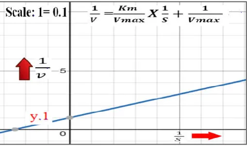
Hans Lineweaver and Dean Burk (1934) suggested the double reciprocal plot for presenting the information in the form of readings or the data on the concentration of substrate [S] and rate or velocity (v) of the biocatalyzed reaction. In enzyme kinetics, double reciprocal plot suggested by Hans Lineweaver and Dean Burk is well esteemed graphical presentation of the data on concentration of the substrate [S] and velocity (v) of the biocatalyzed reaction recognized as, the “Lineweaver–Burk plot”. This plot deserve wide applicability. The most significant application of Lineweaver–Burk plot lies in the determination of concentration of substrate [S] which is responsible for achievement of the half the maximum rate or the velocity (Vmax ÷ 2) of the biochemical reaction catalyzed by the enzymes. The “Km” or Michaelis constant is the concentration of substrate [S] responsible for yield of the reaction rate, which is corresponding to exactly half the rate or velocity of maximal (Vmax ÷ 2) for enzyme involved biochemical reaction. For practical purposes, this “Km” or Constant of Michaelis is the reading pertaining [S] that allows velocity to achieve half with reference to maximum rate or velocity (Vmax). The affinity of enzymes for their substrate vary. Generally, the enzyme with a higher Km value has little bit lower affinity for its substrate. According to Keith J. Laidler (1997), enzymes with lower affinity for their substrate, requires a greater volume of substrate or substrate concentration for the purpose to achieve maximum rate or velocity of enzyme involved biochemical reactions. The wide range of applicability is the distinguishing feature of Lineweaver–Burk plot. In the past, there was no computer facilities as today. In such a critical situation, the parameters of enzyme kinetics, Km and Vmax served a lot through this Lineweaver-Burk plot for fortified concept of enzyme kinetics. In this Lineweaver-Burk plot, reading the inverse of maximum velocity of biocatalyzed reaction (1÷ Vmax) take the position of y-intercept (Fig.1). The negative value of inverse of Km (1÷Km) take the position of x-intercept. The quick visual impression of the inverse form of substrate concentration and rate or velocity of reaction is one more advantage of Lineweaver-Burk plot. And this feature help for understanding the concept of enzyme inhibition. Accordingly, mathematical equation suggested by Lineweaver and Dean Burk (1934) can

be written as: = +

Fig. 1. Regular form of Linrweaver-Burk Plot (Double Reciprocal Plot)

y1= = +

This Lineweaver–Burk plot deserve wide applicability. It is useful for the determination of Km, the most significant factor

in enzyme kinetics. The intercept on y – axis of “Lineweaver– Burk-Plot” is the reciprocal of Vmax or (1/ Vmax). And intercept

on X – axis of “Lineweaver–Burk-Plot” is the reciprocal of -

Km or (−1/Km). Reciprocals of both, [S] and (v) are utilized in

the Lineweaver-Burk plot. That is to say, this plot is pertaining and . Therefore, “Lineweaver–Burk-Plot” is also termed as a double reciprocal graph. This attempt through the “Lineweaver-Burk-Plot”, is giving quick, concept or idea of the biochemical reaction. It also allow to understand the mechanism of activation of enzyme and inhibition of enzyme. Researchers including authors of present attempt designating the double reciprocal plot as a Nobel Plot. Most of researchers entertaining the enzyme kinetics through this double reciprocal plot are non-mathematical academicians. Present attempt is trying it’s best to minimize the errors in understanding the concepts in enzyme kinetics through modification in the “Lineweaver-Burk-Plot”. Each and every method is with positive and negative points of advantages. According to Hayakawa, et al (2006), there is distortion of error structure through this double reciprocal plot of “Lineweaver-Burk-Plot”. It is therefore, method of graphical presentation of “Lineweaver–Burk-Plot” (double-reciprocal-plot) appears to attempt to minimize errors. This may yield easier method of calculation of constants or parameters of enzyme kinetics. On this line of improvement of method of calculation of constants or parameters of enzyme kinetics, much more work is already exist. According to Hayakawa, et al (2006), methods of improvement in the calculation of constants or parameters of enzyme kinetics are under the title, “non-linear regression or alternative linear forms of equations”. And they include: the plot of “Hans-Woolf”; the plot of “Eadie-Hofste”; such and the others (Greco and Hakala, 1979).

Dick (2011) explainedtype of inhibition of enzyme activity or stoping the working of enzymes. Of course, this discussion is based exclusively on “Lineweaver–Burk-Plot” (reciprocals ob both the axes) is able to group or classify the inhibitors of actions of enzymes. Accordingly, the inhibitors of enzyme can basically be grouped into the types like: The “Competitive Inhibitors”; “Non-competitive inhibitors” and “uncompetitive inhibitors”. The inhibitors of enzyme of “Competitive” class deserve one and the same point of intersection on the Y-axis. It clearly means, inhibitors of enzyme of “Competitive” class are not affecting on maximal rate or velocity of reaction (competitive inhibitors provide protection the maximum velocity Vmax . They keep this maximum velocity Vmax non-affected). But, slopes of equations are not same. Slopes are different slopes. The inhibitors of enzyme of “Non-competitive” class deserve one and the same point of intersection on the X-axis. It clearly means, inhibitors of enzyme of “Non-competitive” class are not affecting on the Km, the [S] for half the maximal rate or velocity of reaction (Km is remains unaffected by non-competitive inhibitors. The inverse of Km doesn't change). The non-competitive inhibition produces plots with the same x-intercept (−1/Km) as

(4)

the use of different linear transformation” and listed some problems with Lineweaver–Burk plot (double reciprocal plot). Accordingly, Lineweaver–Burk plot (double reciprocal graph) is appearing in most of the new as well older books of biochemistry. It seems in having prone to error. There may be mistake in understanding the expected for researchers. The readings of inverse of “v” are on Y – axis. The readings of inverse of “[S]” are on X – axis. The lower values of both the readings (inverse of “v” and inverse of “[S]”) are occupying higher (signifiacant) position in graph. And… and… higher values of both the readings (inverse of “v” and inverse of “[S]”) are occupying lower (non-significant) position in graph. Both the conditions may be interpreted wrongly.

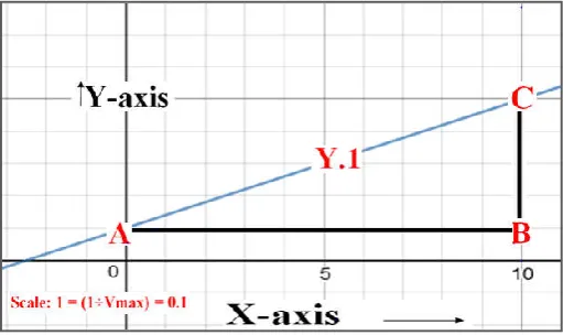
Fig. 2. Right angled triangle through the use of “Regular form of Linrweaver-Burk Plot (Double Reciprocal Plot) (Y.1)

In a Regular form of Linrweaver-Burk Plot (Double Reciprocal Plot) [ y1= (Km÷Vmax) x + (1÷Vmax)]; when the value of x is

one, the y value correspond to [(Km +1)÷Vmax]. The y – intercept of the regular form of Linrweaver-Burk Plot (Double Reciprocal Plot) correspond to (1÷Vmax)]. In figure 2; the y – intercept of the regular form of Linrweaver-Burk Plot (Double Reciprocal Plot) is designated as point: “A”. The co-ordinates of the point “A” are zero and reciprocal of maximum velocity of biochemical reaction involving the interplay of the enzymes. It can be written as: [A (0, 1÷Vmax)]. The line segment perpendicular to y – axis and passing through as point: “A” up to the point: “B” is considered as one of the side of triangle. At the point “B”, x equals to one and y equals to the reciprocal of maximum velocity of biochemical reaction involving the interplay of the enzymes (figure 2). Therefore the co-ordinates of the point “B” can be written as: [A (1, 1÷Vmax). As stated earlier, when the value of x is one, the y value of Regular form of Linrweaver-Burk Plot (Double Reciprocal Plot) (y1)

correspond to: [(Km +1)÷Vmax]. The point (with x – value equals to one) in regular form of Linrweaver-Burk Plot (Double Reciprocal Plot) (y1) claiming the y value is

designated as “C”. The co-ordinates of the point “C” can be written as: C [ 1, (Km +1) ÷Vmax]. Joining the point “A” to the point “B”; the point “B” to the point “C” and the point “C” to “A” yields right angled triangle (figure – 2). A right-angled triangle is a triangle in which measure of one angle is ninety degree (or a right angle).

(B). Geometrical Centroid of Right Angled Triangle:

The relation between the sides and angles of a right angled triangle is the basis for trigonometry. The side opposite the right angle is called the hypotenuse. The sides adjacent to the right angle are called legs. In geometry, the Euler line, named after Leonhard Euler. The Euler line is a line determined from

any triangle that is not equilateral. It is a central line of the triangle, and it passes through several important points determined from the triangle, including the orthocenter, the circumcenter, the centroid, the Exeter point and the center of the nine-point circle of the triangle. The centroid is also called as geometric center of a plane figure. It is the arithmetic mean position of all the points in the figure. Altshiller-Court, Nathan (1925) informally defined the centroid as the point at which a cutout of the shape could be perfectly balanced on the tip of a pin. The barycenter is a synonym used for centroid. The centroid of a triangle is the point of intersection of it’s three medians. It is a point of concurrency of the triangle. It is the point, where all the three medians intersect. It is often described as the center of gravity of triangle. The geometrical properties of centroid of a triangle include: Intersection of the three medians exert to form the centroid; The centroid is one of the points of concurrency of a triangle; The centroid is always located inside the triangle; The centroid divides each median in a ratio of 2:1. The centroid will always be 2/3 of the way along any given median. According to Johnson (1929) and Wells (1991), the geometric centroid (center of mass) of the of a triangle is the point formed through the intersections of the three medians of the triangle. The point of centroid, is therefore also called as the median point. It has equivalent triangle center functions.Orthocenter of triangle is the point of intersection of the altitudes. Each leg in a right triangle forms altitude. In a right-angled triangle, the orthocenter lies at the vertex containing the right angle. Altitude of a triangle is a line segment through a vertex and perpendicular to a line containing the base (the side opposite the vertex). This line containing the opposite side is called as the extended base of altitude. The circumcenter of a triangle is the point of intersections of the three perpendicular bisectors of the sides of that particular triangle intersects. In other words, the point of concurrency of the bisector of the sides of a triangle is called the circumcenter. Every triangle has exactly three medians, one from each vertex, and they all intersect each other at the triangle's centroid. For getting the point of centroid in right angled triangle (∆ ABC) (figure – 2) in present attempt, it is necessary to establish the three medians, one from each vertex.

(B.1). Establishment of the line Y.2 (For one of the median of (∆ ABC) (Fig.3):

Let us first consider the line y2. The slope and intercept on y-

axis of this y2 line are considered as: and

respectively. Therefore, the mathematical equation in “Slope-intercept” form (in the form of typical y= m x +c) of this line y3 can be written as:

Y2 = x +

This equation may also be writte as:

Y2 = x + +

The above equation contain the term: (Km÷Vmax) for two times.

Let us take out one of the term: (Km÷Vmax) as a common factor and let us simplyfy the above equation.

Y2 = [ + ] +

Y2 = [ ] +

(5)

If we replace the “x” by (1÷ S)

Y2 = [ ] +

Let us now substitute the Km = [S (Vmax –v) ÷ v]; the mathematical equation for the line y2 is going to transform

into:

Y2 =

( )

. [ ] +

= ( )( )

+

Simplification will yields into

= ( )( )

+

== ( )( )

It definitely means for plotting the y2; it is necessary to

consider X = (1÷ S) and

Y = ( )( )

Through replacing the values of Vmax; V and S, it is possible to calculate the respective values of Y. This is going to serve the purpose of plotting this new line (y2) along with y1. This

new line (y2) is passing from the point “B” (one of the vertex

of ∆ ABC) and intersecting the line y1 at the point “D” and

dividing the segment AC into two equal parts. Therefore, the segment BD is designated as median of ∆ ABC drawn from the vertex “B” on the side segment “AC”.

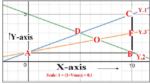
Fig. 3. Line Y.2 as one of the median in Right angled triangle (∆ ABC)

Let us consider the line y3 (Fig.4). The slope and intercept on

y- axis of this y3 line are considered as: and

Y2 = x +

If we replace the “x” by (1÷ S) and substitute the Km = [S (Vmax –v) ÷ v]; the mathematical equation for the line y2 is

going to transform into:

= ( ) +

Simplification of this equation is going to yields into

= ( )

+

=

Y =

Through replacing the values of Vmax; V and S, it is possible to calculate the respective values of Y. This is going to serve the purpose of plotting this new line (y3) along with y1 and y2

This new line (y3) is passing from the point “A” (one of the

vertex of ∆ ABC) and attain half the measurement of the segment “BC” at point “F”. The line (y3) is dividing the

segment BC into two equal parts. Therefore, the segment “AF” is designated as median of ∆ ABC drawn from the vertex “A” on the side segment “BC”.

Fig. 4. Line Y.2 and Y.3 as the two medians in Right angled triangle (∆ ABC)

Let us now consider the line y4 (Fig.5). The slope and intercept

on y- axis of this y4 line are considered as: and

( )

Y4 = x -

If we replace the “x” by (1÷ S) and substitute the Km = [S (Vmax –v) ÷ v]; the mathematical equation for the line y4 is

going to transform into:

= ( )

-

[ ( ) ]

(6)

Simplification of this equation is going to yields into

= ( ) - [ ( ) ]

= ( ) [ ( ) ]

= [( )][( )]

Y = [( )][( )]

Through replacing the values of Vmax; V and S, it is possible to calculate the respective values of Y. This is going to serve the purpose of plotting this new line (y4) along with y1 ; y2 and

y3. This new line (y4) is passing from the point “C” (one of the

vertex of ∆ ABC) and attain half the measurement of the segment “AB” at point “E”. The line (y4) is dividing the

segment AB into two equal parts. Therefore, the segment “CE” is designated as median of ∆ ABC drawn from the vertex “B” on the side segment “AB”. The three medians of right angled triangle in Figure – 5 (and Figure – 6 too) are intersecting at a common point “O”.

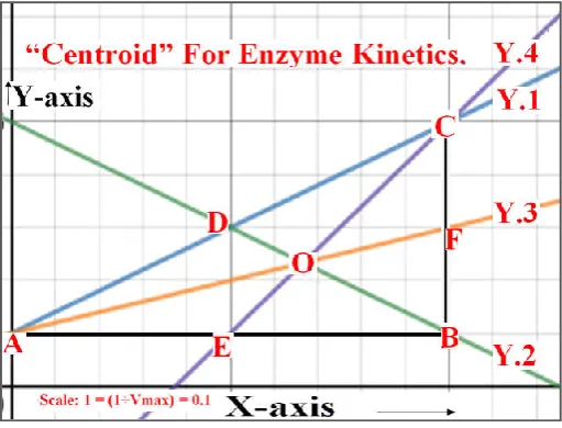
Fig. 5. Centroid (The point “O”) of Right angled triangle (∆ ABC) with (Real Form of Lineweaver-Burk Plot); line Y.2 (First

Median); Y.3 (Second Median) and Y.4 (Third Median)

(B.4). Establishment of Centroid (The point “O”) of Right angled triangle (∆ ABC) obtained through the Linewever-Burk Plot (line Y.1):

In a right angled triangle (∆ ABC) in figure 5, measure of angle “B” is ninety. The segment AB and segment BC are the two perpendicular sides. The segment AC is hypotenuse of a right angled triangle (∆ ABC) in figure 5. The line segment BD is a median of a right angled triangle. It is joining a vertex “B” to the midpoint of the opposite side (line segment AC), thus bisecting that side. The line segment AF is a median of a right angled triangle in figure 5. It is joining a vertex “A” to the midpoint of the opposite side (line segment BC), thus bisecting that side. The line segment CE is a median of a right angled triangle in Figure 5. It is joining a vertex “C” to the midpoint of the opposite side (line segment AB), thus bisecting that side.

The median of a triangle is a line segment joining a vertex to the midpoint of the opposite side, thus bisecting that side. Every triangle has exactly three medians, one from each vertex, and they all intersect each other at the triangle's centroid. In a right angled triangle in figure 5, the point “O” is the median, the x and y– coordinates of which correspond to: 2÷3 and [(Km +1) ÷ 3 Vmax] respectively.

(C). Establishment of Geometrical Orthocenter of Right

Angled Triangle:

Altitude of a triangle is a line segment through a vertex and perpendicular to the line containing the base. The base segment of triangle is the side opposite the vertex. The line containing the opposite side is called the extended base of the altitude. The intersection of the extended base and the altitude is called the foot of the altitude. The length of the altitude, often simply called "the altitude". It is the distance between the extended base and the vertex. The process of drawing the altitude from the vertex to the foot is known as dropping the altitude at that vertex. Altitudes a triangle can be used in the computation of the area of a triangle. One half of the product of length of base and length of altitude equals the area of the triangle. The longest altitude is perpendicular to the shortest side of the triangle. The altitudes are also related to the sides of the triangle through the trigonometric functions (Mitchell, Douglas W. 2005). The three (possibly extended) altitudes intersect in a single point, called the orthocenter of the triangle. The orthocenter lies inside the triangle if and only if the triangle is acute (i.e. does not have an angle greater than or equal to a right angle). If one angle is a right angle, the orthocenter coincides with the vertex at the right angle (Dorin Andrica and Dan S ̧ tefan Marinescu, 2017).

(7)

point “B” in the right angled triangle (∆ ABC) (Fig. 5 and Fig. 6) is claiming the intersection of the line segment AB and the line segment AC. Therefore, the point “B” in the right angled triangle (∆ ABC) (Fig. 5 and Fig. 6) is designated as the orthocenter.

(D). Establishment of Geometrical Circumcenter of Right

Angled Triangle:

According to Smith, Geoff and Leversha, Gerry (2007) the perpendicular bisectors of the sides of a triangle are concurrent (they intersect in one common point). The point of concurrency of the perpendicular bisectors of the sides is called the circumcenter of the triangle. The point of concurrency is not necessarily inside the triangle. It may actually be in the triangle, on the triangle, or outside of the triangle. The perpendicular bisectors of the sides of the triangles do not necessarily pass through the vertices of the triangles. A circumscribed circle is a circle around the outside of a figure passing through all of the vertices of the figure, in the present attempt, passing through the three vertices of the right angled triangle (∆ ABC) (Fig. 5). Since the radii of the circle are congruent, a circumcenter is equidistant from vertices of the triangle. In a right angled triangle, the perpendicular bisectors intersect on the hypotenuse. Since the center of the circumscribed circle lies on the hypotenuse, the hypotenuse becomes the diameter of the circle Richinick, Jennifer (2008).

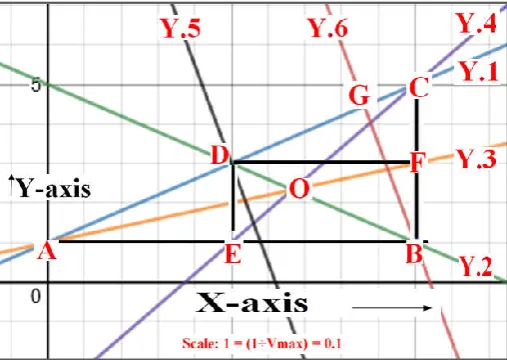
Fig. 6. Circumcenter (The point “D”) of Right angled triangle (∆ ABC) with (Real Form of Lineweaver-Burk Plot: Y.1); line Y.2 (First Median); Y.3 (Second Median); Y.4 (Third Median); Y.5 (Perpendicular Bisectors)

and Y.6 (Altitude)

(E). Establishment of Geometrical Euler line for the Right Angled Triangle Resulted through the use of

Lineweaver-Burk plot:

In geometry, the Euler line, named after Leonhard Euler is a line determined from any triangle that is not equilateral. According to Fraser, Craig G. (2005), Leonhard Euler (15 April, 1707 – 18 September, 1783) was a Swiss mathematician, physicist, astronomer, geographer, logician and engineer. He made important and influential discoveries in many branches of mathematics, such as infinitesimal calculus and graph theory, while also making pioneering contributions to several branches such as topology and analytic number theory. He also introduced much of the modern mathematical terminology and notation, particularly for mathematical

analysis, such as the notion of a mathematical function. He is also known for his work in mechanics, fluid dynamics, optics, astronomy and music theory (Thiele, Rüdiger, 2005). Euler was one of the most eminent mathematicians of the eighteenth century and is held to be one of the greatest in history. He is also widely considered to be the most prolific mathematician of all time. His collected works fill 92 volumes, more than anyone else in the field. He spent most of his adult life in Saint Petersburg, Russia, and in Berlin, then the capital of Prussia (Sandifer, C. Edward, 2007). The Euler line is a central line of the triangle, and it passes through several important points determined from the triangle, including the orthocenter, the circumcenter, the centroid, the exeter point and the center of the nine-point circle of the triangle. The concept of a triangle's Euler line extends to the Euler line of other shapes, such as the quadrilateral and the tetrahedron (Kimberling Clark, 1998). Eulers line is quite popular when one is dealing with geometry. It is a special line in the plane of the triangle that passes through many important well known points. It is proving all those points to be collinear. The collinearity of points is very useful in solving certain complex pure geometry problems. Let us shift our discussion to the present attempt on Establishment of Euler’s Line for Enzyme Kinetics. For this purpose, the Fig. 5 and Fig. 6 in the present attempt are going to serve a lot. In the Fig. 5 and Fig. 6, the line Y.1 is real form of Lineweaver-Burk plot with mathematical equation: y = (Km ÷ Vmax) x + (1÷Vmax). The line segment AB; the line segment BC and the line segment CA are considered for right angled triangle (∆ ABC) resulted through consideration of real form of Lineweaver-Burk plot. According to Kimberling Clark (1998), the Euler line is a central line of the triangle, and it passes through important points determined from the triangle, including the centroid, the orthocenter and the circumcenter.

RESULTS AND DISCUSSION

According to Leonhard Euler (1767), the orthocenter, circumcenter and centroid of any triangle are collinear. This unique property of triangle is also true for total nine points of center of triangle. These other six points of center of triangle had not been defined in Euler's time. Other notable points concerned with a triangle and lie on the Euler line include: de Longchamps point, Schiffler point, Exeter point, and Gossard perspector. The tangential triangle of a reference triangle is tangent to the latter's circumcircle at the reference triangle's vertices. The circumcenter of the tangential triangle lies on the Euler line of the reference triangle. The center of similitude of the orthic and tangential triangles is also on the Euler line. The results of the present are explained away through the points like: Centroid for Enzyme Kinetics; Orthocenter for Enzyme Kinetics; Circumcenter for Enzyme Kinetics and Euler Line for Enzyme Kinetics.

Centroid for Enzyme Kinetics

(8)

correspond to: y = - (Km ÷ Vmax )x + [(Km+1)÷Vmax]. The line Y.2 is passing through the point vertex “B” and the midpoint of hypotenuse (midpoint: “D” on line segment: AC). The line Y.3 is with positive slope correspond to: (Km ÷ 2 Vmax) and y – intercept correspond to: [1÷Vmax]. The mathematical equation for line Y.3 correspond to: y = (Km ÷ 2Vmax) x + [1÷Vmax]. The line Y.3 is passing through the point vertex “A” and the midpoint of the vertical side of right angled triangle (∆ ABC) (midpoint: “F” on line segment: BC). The line Y.4 is with positive slope correspond to: (2Km ÷ Vmax) and y – intercept correspond to: [(Km – 1) ÷ Vmax ]. The mathematical equation for line Y.4 correspond to: y = (2Km ÷ Vmax) x + [(Km-1)÷Vmax]. The line Y.4 is passing through the point vertex “C” and the midpoint of the horizontal side of right angled triangle (∆ ABC) (midpoint: “E” on line segment: AB). All the three line segments representing medians of right angled triangle (∆ ABC) (line segment: BD; line segment: AF and line segment: CE) are intersecting the common point: “O”. Therefore, the point: “O” inside the right angled triangle (∆ ABC) is considered as the centroid. The x- ordinate of the point “O” correspond to: (2÷3). The y- co-ordinate of the point “O” correspond to: [(Km+3) ÷ (3 Vmax)]. This point “O” with co-ordinates: (2÷3) and [(Km+3) ÷ (3 Vmax)], herewith labeled as “Centroid for Enzyme Kinetics”. The line segment (BD) representing median drawn to the hypotenuse has the measure half the hypotenuse (line segment AC).

Orthocenter for Enzyme Kinetics

According to Douglas W. (2005), the three (possibly extended) altitudes intersect in a single point, called the orthocenter of the triangle. The orthocenter lies inside the triangle if and only if the triangle is acute (i.e. does not have an angle greater than or equal to a right angle). If one angle is a right angle, the orthocenter coincides with the vertex at the right angle (Dorin Andrica and Dan S ̧ tefan Marinescu, 2017). An altitude of a triangle is a line segment through a vertex and perpendicular to a line containing the base (the side opposite the vertex). This line containing the opposite side is called the extended base of the altitude. The length of the altitude, often simply called "the altitude", is the distance between the extended base and the vertex. The process of drawing the altitude from the vertex to the foot is known as dropping the altitude at that vertex. It is a special case of orthogonal projection (Bryant and Bradley, 1998). In the Fig. 5 and Fig. 6, the line segment: CB is the altitude through a vertex (the point: “C”) and perpendicular to the line segment: AB. In the Fig. 5 and Fig. 6, the line segment: AB is the altitude through a vertex (the point: “A”) and perpendicular to the line segment: BC. In the Fig. 6, the “line segment: BG” on line Y.6 is representing the third altitude. The slope of line Y.6 is minus (Vmax ÷Km). The intercept of line Y.6 on y – axis correspond to: [(Km+Vmax2) ÷ (KmVmax)]. The mathematical equation for line Y.6 can be written as:

Y6 = x +

.

All the three altitudes of right angled triangle (∆ ABC) (line segment: AB; line segment: CB and line segment: BG) (Fig. 6) are intersecting the common point: “B”. Therefore, the point: “B” of the right angled triangle (∆ ABC) is considered as the orthocenter. The x- co-ordinate of the point “B” correspond to: 1. The y- co-ordinate of the point “B” correspond to: [(1 ÷

Vmax)]. This point “B” with co-ordinates: (1) and [(1 ÷ Vmax)], herewith labeled as “Orthocenter for Enzyme Kinetics”.

Circumcenter for Enzyme Kinetics

The perpendicular bisectors of the sides of a triangle are concurrent (they intersect in one common point). The point of concurrency of the perpendicular bisectors of the sides is called the circumcenter of the triangle (Smith, Geoff and Leversha, Gerry, 2007). The point of concurrency is not

necessarily inside the triangle. It may actually be in the

triangle, on the triangle, or outside of the triangle. The perpendicular bisectors of the sides of the triangles do not necessarily pass through the vertices of the triangles. A circumscribed circle is a circle around the outside of a figure passing through all of the vertices of the figure, in the present attempt, passing through the three vertices of the right angled triangle. Since the radii of the circle are congruent, a circumcenter is equidistant from vertices of the triangle. In a right angled triangle, the perpendicular bisectors intersect on the hypotenuse. Since the center of the circumscribed circle lies on the hypotenuse, the hypotenuse becomes the diameter of the circle Richinick, Jennifer (2008).

In the Fig. 6, the line Y.5 is representing the bisector of hypotenuse (line segment: AC). The slope of line Y.5 is minus (vmax ÷Km). The intercept of line Y.5 on y – axis correspond to: [(km2+2Km+Vmax2) ÷ 2KmVmax].

Y5 = x +

. .

.

In the Fig. 5 and Fig. 6, the line segment DF is the bisector of the line segment BC of the right angled triangle (∆ ABC). In the Fig. 5 and Fig. 6, the line segment DE is the bisector of the line segment AB of the right angled triangle (∆ ABC). The three bisectors (bisector line segment DE; bisector line segment DF and the line Y.5) are intersecting at a common point: “D”. Therefore, the point: “D” of the right angled triangle (∆ ABC) is considered as the circumcenter. The lengths of line segment BD; line segment AD and line segment CD are equal. According to Euler, Leonhard (1767), the circumcenter is equidistant from the three vertices of the triangle and lies on the perpendicular bisector. The x- ordinate of the point “D” correspond to: (1÷2). The y- co-ordinate of the point “B” correspond to: [(Km+2) ÷ 2Vmax]. This point “D” with co-ordinates: (1÷2) and [(Km+2) ÷ 2Vmax], herewith labeled as “Circumcenter for Enzyme Kinetics”.

Euler Line for Enzyme Kinetics

Euler line, named after Leonhard Euler. The Euler line is a line determined from any triangle that is not equilateral. It is a central line of the triangle, and it passes through several important points determined from the triangle, including the orthocenter, the circumcenter, the centroid, the Exeter point and the center of the nine-point circle of the triangle. The orthocenter, the circumcenter and the centroid are the three “centers” of the triangle lie on one straight line, called the Euler line. The point with co-ordinates: (2÷3) and [(Km+3) ÷ (3 Vmax)] in Lineweaver-Burk plot is “Centroid for Enzyme Kinetics” (The point: “O” in Fig. 5 and 6).

(9)

The point with co-ordinates: (1) and [(1 ÷ Vmax)] in Lineweaver-Burk plot is “Orthocenter” for Enzyme Kinetics” (The point: “B” in Fig. 5 and 6). The point with co-ordinates: (1÷2) and [(Km+2) ÷ Vmax] in Lineweaver-Burk plot is “Circumcenter” for Enzyme Kinetics” (The point: “D” in Fig. 5 and 6). The line passing through the point of centroid (The point: “O” in Fig. 5 and 6); Orthocenter (The point: “B” in Fig. 5 and 6) and Circumcenter (The point: “D” in Fig. 5 and 6) of right angled triangle resulted through Lineweaver-Burk plot is named herewith as: “Euler Line for Enzyme Kinetics”.

Properties of Euler Line for Enzyme Kinetics

1. Lineweaver-Burk plot (double reciprocal plot) and Euler Line for Enzyme Kinetics are with equal and opposite slope. Lineweaver-Burk plot (double reciprocal plot) is with positive value of (Km÷Vmax) as a slope. Euler Line for Enzyme Kinetics is with negative value of (Km÷Vmax) as a slope.

2. The intercept on y-axis for Lineweaver-Burk plot (double reciprocal plot) for Enzyme Kinetics correspond to: (1 ÷ Vmax). The intercept on y-axis for Euler Line for Enzyme Kinetics correspond to: [(Km +2) ÷ Vmax)].

3. Lineweaver-Burk plot (double reciprocal plot) and Euler Line for Enzyme Kinetics are intersecting at the point, x – co-ordinate of which correspond to: (1÷2) and y- co-ordinate of which correspond to: [(Km+2) ÷ Vmax].

4. The centroid for enzyme kinetics is always located between the orthocenter and the circumcenter of enzyme kinetics.

5. The distance from the centroid (for enzyme kinetics) to the orthocenter (for enzyme kinetics) is always twice the distance from the centroid (for enzyme kinetics) to the circumcenter (for enzyme kinetics).

6. The line segment (BD) (of line: Y.2) representing median drawn to the hypotenuse has the measure half the hypotenuse (line segment AC) (of line: Y.1).

Conclusion

In a Regular form of Linrweaver-Burk Plot (Double Reciprocal Plot) [ y1= (Km÷Vmax) x + (1÷Vmax)]; when the value of x is

one, the y value correspond to [(Km +1)÷Vmax]. The y – intercept of the regular form of Linrweaver-Burk Plot (Double Reciprocal Plot) correspond to (1÷Vmax)]. The y – intercept of the regular form of Linrweaver-Burk Plot (Double Reciprocal Plot) is designated as point: “A”. The co-ordinates of the point “A” are zero and reciprocal of maximum velocity of biochemical reaction involving the interplay of the enzymes. It can be written as: [A (0, 1÷Vmax). The line segment perpendicular to y – axis and passing through point: “A” up to the point: “B” is considered as one of the side of triangle. At the point “B”, x equals to one and y equals to the reciprocal of maximum velocity of biochemical reaction involving the interplay of the enzymes. The co-ordinates of the point “B” can be written as: [A (1, 1÷Vmax). The point with x – value equals to one and y – equals to [(Km +1) ÷Vmax] in regular form of Linrweaver-Burk Plot (Double Reciprocal Plot) is designated as “C”. The co-ordinates of the point “C” can be written as: C [ 1, (Km +1) ÷Vmax]. Joining the point “A” to the point “B”; the point “B” to the point “C” and the point “C” to “A” yields right angled triangle. The point with co-ordinates: (2÷3) and [(Km+3) ÷ (3 Vmax)] in

Lineweaver-Burk plot is “Centroid for Enzyme Kinetics”. The point with co-ordinates: (1) and [(1 ÷ Vmax)] in Lineweaver-Burk plot is “Orthocenter” for Enzyme Kinetics”. The point with co-ordinates: (1÷2) and [(Km+2) ÷ Vmax] in Lineweaver-Burk plot is “Circumcenter” for Enzyme Kinetics”. The line passing through the point of centroid; Orthocenter and Circumcenter of right angled triangle resulted through Lineweaver-Burk plot is named herewith as: “Euler Line for Enzyme Kinetics”. Lineweaver-Burk plot (double reciprocal plot) and Euler Line for Enzyme Kinetics are with equal and opposite slope. Lineweaver-Burk plot (double reciprocal plot) is with positive value of (Km÷Vmax) as a slope. Euler Line for Enzyme Kinetics is with negative value of (Km÷Vmax) as a slope. The intercept on y-axis for Lineweaver-Burk plot (double reciprocal plot) for Enzyme Kinetics correspond to: (1 ÷ Vmax). The intercept on y-axis for Euler Line for Enzyme Kinetics correspond to: [(Km +2) ÷ Vmax)]. Lineweaver-Burk plot (double reciprocal plot) and Euler Line for Enzyme Kinetics are intersecting at the point, x – co-ordinate of which correspond to: (1÷2) and y- co-ordinate of which correspond to: [(Km+2) ÷ Vmax]. The centroid for enzyme kinetics is always located between the orthocenter and the circumcenter of enzyme kinetics. The distance from the centroid to the orthocenter is always twice the distance from the centroid to the circumcenter.

Acknowledgements

31 December is the birthday of Hon. Dr. Avram Hershko (Hungarian-born Israeli biochemist and Nobel laureate). His kind self is well known for ubiquitin mediated degradation of the proteins. Through the best compliments from India, the present attempt is wishing Hon. Dr. Avram Hershko Happy Birthday. Academic support and inspiration received from the Agricultural Development Trust, Baramati for the present studies exert a grand salutary influence.

REFERENCES

"Geometry classes, Problem 331. Square, Point on the Inscribed Circle, Tangency Points. Math teacher Master Degree. College, SAT Prep. Elearning, Online math tutor, LMS". gogeometry.com. Retrieved 2017-12-12.

"Maths is Fun - Can't Find It (404)". www.mathsisfun.com. Retrieved 2017-12-12.

"Problem Set 1.3". jwilson.coe.uga.edu. Retrieved 2017-12-12.

Altshiller-Court, Nathan 1925. College Geometry: An Introduction to the Modern Geometry of the Triangle and the Circle (2nd ed.), New York: Barnes & Noble,

LCCN52013504. https://en.wikipedia.org/wiki/Centroid Berg, Jeremy M., Tymoczko, John L., Stryer, Lubert 2002.

"The Michaelis-Menten Model Accounts for the Kinetic Properties of Many Enzymes". Biochemistry. 5th edition. W H Freeman.

Bibcode:1988Sci...241.1620K. doi:10.1126/science.241.4873. 1620. PMID 17820893.

Briggs GE, Haldane JB. 1925. "A Note on the Kinetics of Enzyme Action". The Biochemical Journal, 19 (2): 339– 339. doi:10.1042/bj0190338. PMC 1259181. PMID 16743508.

Briggs, William; Cochran, Lyle, 2011. Calculus / Early Transcendentals Single Variable. Addison-Wesley.

(10)

Bryant, V., and Bradley, H. 1998. "Triangular Light Routes," Mathematical Gazette 82, July 1998, 298-299. https://en.wikipedia.org/wiki/Altitude_(triangle).

Callahan BP, Miller BG (December 2007). "OMP decarboxylase. An enigma persists". Bioorganic Chemistry,

35 (6): 465–9. doi:10.1016/j.bioorg.2007.07.004. PMID 17889251.

Chakerian, G.D. "A Distorted View of Geometry." Ch. 7 in Mathematical Plums (R. Honsberger, editor). Washington, DC: Mathematical Association of America, 1979: 147. Clark, W. E. and Suen, S. "An Inequality Related to Vizing's

Conjecture." Electronic J. Combinatorics 7, No. 1, N4, 1-3, 2000. http://www.combinatorics.org/Volume_7/Abstracts/ v7i1n4.html.

Coxeter, H. S. M. and Greitzer, S. L. Geometry Revisited. Washington, DC: Math. Assoc. Amer., p. 84, 1967.

Darvasi, Gyula (March 2005), "Converse of a Property of Right Triangles", The Mathematical Gazette, 89 (514): 72– 76. https://en.wikipedia.org/wiki/Right_triangle

Detemple, D. and Harold, S. "A Round-Up of Square Problems." Math. Mag. 69, 15-27, 1996.

Devlin, Keith J. 2004. Sets, Functions, and Logic / An Introduction to Abstract Mathematics (3rd ed.). Chapman & Hall / CRC Mathematics. ISBN978-1-58488-449-1.

Dick RM (2011). "Chapter 2. Pharmacodynamics: The Study of Drug Action". In Ouellette R, Joyce JA. Pharmacology for Nurse Anesthesiology. Jones & Bartlett Learning. ISBN978-0-7637-8607-6

Dixon, R. Mathographics. New York: Dover, p. 16, 1991.Eppstein, D. "Rectilinear Geometry."http://www. ics.uci.edu/~eppstein/junkyard/rect.html.

Dorin Andrica and Dan S ̧ tefan Marinescu (2017). New Interpolation Inequalities to Euler’s R ≥ 2r. Forum Geometricorum, Volume 17 (2017), pp. 149–156.

Dowd, John E.; Riggs, Douglas S. (1965). "A comparison of estimates of Michaelis–Menten kinetic constants from various linear transformations" (pdf). Journal of Biological Chemistry. 240 (2): 863–869.

Ellis RJ (October 2001). "Macromolecular crowding: obvious but underappreciated". Trends in Biochemical Sciences. 26 (10): 597–604. doi:10.1016/S0968- 0004(01)01938-7. PMID 11590012.

Euler, Leonhard (1767). "Solutio facilis problematum quorundam geometricorum difficillimorum" [Easy solution of some difficult geometric problems]. Novi Commentarii Academiae Scientarum Imperialis Petropolitanae. 11: 103– 123. E325. Reprinted in Opera Omnia, ser. I, vol. XXVI, pp. 139–157, Societas Scientiarum Naturalium Helveticae, Lausanne, 1953, MR0061061.

Fischer, G. (Ed.). Plate 1 in Mathematische Modelle aus den Sammlungen von Universitäten und Museen, Bildband. Braunschweig, Germany: Vieweg, p. 2, 1986.

Fletcher, Peter; Patty, C. Wayne (1988). Foundations of Higher Mathematics. PWS-Kent.ISBN0-87150-164-3.

Fraser, Craig G. (11 February 2005). Leonhard Euler's 1744 book on the calculus of variations. ISBN 978-0-08-045744-4. In Grattan-Guinness 2005, pp. 168–80.

Fukagawa, H. and Pedoe, D. "One or Two Circles and Squares," "Three Circles and Squares," and "Many Circles and Squares (Casey's Theorem)." §3.1-3.3 in Japanese Temple Geometry Problems. Winnipeg, Manitoba, Canada: Charles Babbage Research Foundation, pp. 37-42 and 117-125, 1989.

Gardner, M. The Sixth Book of Mathematical Games from Scientific American. Chicago, IL: University of Chicago Press, pp. 165 and 167, 1984.

Greco, W.R.; Hakala, M.T. (1979). "Evaluation of methods for estimating the dissociation constant of tight binding enzyme inhibitors" (PDF). Journal of Biological Chemistry. 254 (23): 12104–12109. PMID500698.

Greco, W.R.; Hakala, M.T. (1979). "Evaluation of methods for estimating the dissociation constant of tight binding enzyme inhibitors,".J BiolChem254 (23): 12104–12109. PMID 500698.

Guy, R. K. "Rational Distances from the Corners of a Square." §D19 in Unsolved Problems in Number Theory, 2nd ed. New York: Springer-Verlag, pp. 181-185, 1994.

Hall, Arthur Graham; Frink, Fred Goodrich (January 1909). "Chapter II. The Acute Angle [14] Inverse trigonometric functions". Written at Ann Arbor, Michigan, USA.

Trigonometry. Part I: Plane Trigonometry. New York,

USA: Henry Holt and Company / Norwood Press / J. S. Cushing Co. - Berwick & Smith Co., Norwood, Massachusetts, USA. p. 15. Retrieved 2017-08-12.

https://en.wikipedia.org/wiki/Inverse_function

Harris, J. W. and Stocker, H. "Square." §3.6.6 in Handbook of Mathematics and Computational Science. New York: Springer-Verlag, pp. 84-85, 1998.

Hayakawa, K.; Guo, L.; Terentyeva, E.A.; Li, X.K.; Kimura, H.; Hirano, M.; Yoshikawa, K.; Nagamine, T.; et al. (2006). "Determination of specific activities and kinetic constants of biotinidase and lipoamidase in LEW rat and Lactobacillus casei (Shirota)". Journal of Chromatography B. 844 (2): 240–50. doi:10.1016/j.jchromb.2006.07.006.

PMID16876490.

Hayakawa, K.; Guo, L.; Terentyeva, E.A.; Li, X.K.; Kimura, H.; Hirano, M.; Yoshikawa,K.; Nagamine, T. et al. (2006). "Determination of specific activities and kinetic constants of biotinidase and lipoamidase in LEW rat and Lactobacillus casei (Shirota)". J Chromatogr B AnalytTechnol Biomed Life Sci844 (2): 240– 50.doi:10.1016/j.jchromb.2006.07.006. PMID 16876490. http://forumgeom.fau.edu/FG2017volume17/FG201719.pdf https://en.wikipedia.org/wiki/Euler_line

John E. Dowd and Douglas Briggs (1965). Estimates of Michaelis – Menten kinetic constants from various linear transformation. The Journal of Biological Chemistry Vol. 240 No. 2 February, 1965. http://www.jbc.org/content/240 /2/863.full.pdf

John H. Conway, Heidi Burgiel, Chaim Goodman-Strauss, (2008) The Symmetries of Things, ISBN 978-1-56881-220-5 (Chapter 20, Generalized Schaefli symbols, Types of symmetry of a polygon pp. 275-278).

Johnson, R. A. Modern Geometry: An Elementary Treatise on the Geometry of the Triangle and the Circle. Boston, MA: Houghton Mifflin, pp. 173-176, 249-250, and 268-269, 1929. Darvasi, Gyula (March 2005), "Converse of a Property of Right Triangles", The Mathematical Gazette, 89 (514): 72–76.

Josefsson, Martin, "Properties of equidiagonal quadrilaterals" Forum Geometricorum, 14 (2014), 129-144.

Keisler, Howard Jerome. "Differentiation" (PDF). Retrieved 2015-01-24. §2.4

Keith J. Laidler (1997). New Beer in an Old Bottle: Eduard Buchner and the Growth of Biochemical Knowledge, pp. 127–133, ed. A. Cornish-Bowden, Universitat de València, Valencia, Spain, 1997 http://bip.cnrs-mrs.fr/bip10/newbeer/ laidler.pdf

(11)

Kern, W. F. and Bland, J. R. Solid Mensuration with Proofs, 2nd ed. New York: Wiley, p. 2, 1948.

Kimberling, Clark (1998). "Triangle centers and central triangles". Congressus Numerantium. 129: i–xxv, 1–295. Kopelman R (September 1988). "Fractal reaction kinetics".

Science. 241 (4873): 1620

Korn, Grandino Arthur; Korn, Theresa M. (2000) [1961]. "21.2.-4. Inverse Trigonometric Functions". Mathematical handbook for scientists and engineers: Definitions, theorems, and formulars for reference and review (3 ed.). Mineola, New York, USA: Dover Publications, Inc.

p. 811;. ISBN978-0-486-41147-7.

Lay, Steven R. (2006). Analysis / With an Introduction to Proof (4 ed.). Pearson / Prentice Hall. ISBN 978-0-13-148101-5.

Leskovac, V. (2003). Comprehensive enzyme kinetics. New York: Kluwer Academic/Plenum Pub. ISBN 978-0-306-46712-7.

Lineweaver, H; Burk, D. (1934). "The determination of enzyme dissociation constants". Journal of the American

Chemical Society. 56 (3): 658–666.

doi:10.1021/ja01318a036.

Martin Lundsgaard Hansen, thats IT (c). "Vagn Lundsgaard Hansen". www2.mat.dtu.dk Retrieved 2017-12-12.

Michaelis L, Menten M (1913). "Die Kinetik der Invertinwirkung" [The Kinetics of Invertase Action]. Biochem. Z. (in German). 49: 333–369.; Michaelis L, Menten ML, Johnson KA, Goody RS (2011). "The original Michaelis constant: translation of the 1913 Michaelis-Menten paper". Biochemistry. 50 (39): 8264– 9. doi:10.1021/bi201284u. PMC 3381512. PMID 21888353. Mitchell, Douglas W. (2005). A Heron-type formula for the

reciprocal area of a triangle. Mathematical Gazette 89, November 2005, 494. https://en.wikipedia.org/ wiki/Altitude_(triangle)

Oldham, Keith B.; Myland, Jan C.; Spanier, Jerome (2009) [1987]. An Atlas of Functions: with Equator, the Atlas Function Calculator (2 ed.). Springer Science+Business Media, LLC. doi:10.1007/978-0-387-48807-3. ISBN 978-0-387-48806-6. LCCN2008937525.

Park, Poo-Sung. "Regular polytope distances", Forum Geometricorum 16, 2016, 227-232. http://forumgeom.fau. edu/FG2016volume16/FG201627.pdf

Radzicka A, Wolfenden R (January 1995). "A proficient

enzyme". Science. 267 (5194): 90–931.

Bibcode:1995Sci...267...90R.

doi:10.1126/science.7809611. PMID 7809611.

Richinick, Jennifer (2008). The upside-down Pythagorean Theorem," Mathematical Gazette 92, July 2008, 313–317. https://en.wikipedia.org/wiki/Altitude_(triangle).

Sandifer, C. Edward (2007). The Early Mathematics of Leonhard Euler. Mathematical Association of America. ISBN978-0-88385-559-1.

Scheinerman, Edward R. (2013). Mathematics: A Discrete

Introduction. Brooks/Cole. p. 173. ISBN978-0840049421.

Scheinerman, Edward R. (2013). Mathematics: A Discrete Introduction. Brooks/Cole. p. 173.ISBN978-0840049421.

Schomburg I, Chang A, Placzek S, Söhngen C, Rother M, Lang M, Munaretto C, Ulas S, Stelzer M, Grote A, Scheer M, Schomburg D (January 2013). "BRENDA in 2013: integrated reactions, kinetic data, enzyme function data, improved disease classification: new options and contents in BRENDA". Nucleic Acids Research. 41 (Database issue): D764–72. doi:10.1093/nar/gks1049. PMC 3531171. PMID 23203881

Seema Karna Dongare, Manali Rameshrao Shinde, Vitthalrao Bhimasha Khyade (2018). Mathematical Inverse Function (Equation) For Enzyme Kinetics. Research Journal of Recent Sciences. Res. J. Recent Sci. Vol. 7(12), 9-15, December (2018). www.isca.in, www.isca.me

Seema Karna Dongare, Manali Rameshrao Shinde, Vitthalrao Bhimasha Khyade (2018). Mathematical Inverse Function (Equation) For Enzyme Kinetics. International Journal of Scientific Research in Chemistry (IJSRCH) | Online ISSN: 2456-8457 © 2018 IJSRCH | Volume 3 | Issue 4: 35– 42. http://ijsrch.com/archive.php?v=3&i=6&pyear=2018 Segel, L.A.; Slemrod, M. (1989). "The quasi-steady-state

assumption: A case study in perturbation". ThermochimActa31 (3): 446–477. doi:10.1137/1031091. Smith, Douglas; Eggen, Maurice; St. Andre, Richard (2006). A

Transition to Advanced Mathematics (6 ed.). Thompson Brooks/Cole. ISBN978-0-534-39900-9.

Smith, Geoff and Leversha, Gerry (2007). Euler and triangle geometry", Mathematical Gazette 91, November 2007, 436–452.

Stryer L, Berg JM, Tymoczko JL (2002). Biochemistry (5th ed.). San Francisco: W.H.Freeman. ISBN 0-7167-4955-6. Tabachnikov, Serge; Tsukerman, Emmanuel (May 2014),

"Circumcenter of Mass and Generalized Euler Line", Discrete and Computational Geometry, 51 (51): 815–836, arXiv:1301.0496, doi:10.1007/s00454-014-9597-2. Thiele, Rüdiger (2005). The mathematics and science of

Leonhard Euler. In Kinyon, Michael; van Brummelen, Glen (eds.). Mathematics and the Historian's Craft: The Kenneth O. May Lectures. Springer. pp. 81–140. ISBN978-0-387-25284-1.

Thomas, Jr., George Brinton (1972). Calculus and Analytic Geometry Part 1: Functions of One Variable and Analytic Geometry (Alternate ed.).Addison-Wesley.

V. B. Khyade (2018). Inverse Form of Equation For Lineweaver-Burk Plot for Enzyme Kinetics. Eureka (An International Journal of Mathematics) Volume 5 December, 2018. ISSN 2392-4233.

Vitthalrao B. Khyade; Vivekanand V. Khyade and Sunanda V. Khyade (2017). The Baramati Quotient for the accuracy in calculation of Km value for Enzyme Kinetics. International Academic Journal of Innovative Research Vol. 4, No. 1, 2017, pp. 1-22.ISSN 2454-390X www.iaiest.com

Weisstein, W., Eric. "Square". mathworld. http://mathworld.wolfram.com/Square.htmlWeisstein, Eric W. "Square." From MathWorld--A Wolfram Web Resource. http://mathworld.wolfram.com/Square.html Wells, Christopher J."Quadrilaterals". www.technologyuk.net.

Retrieved 2017-12-12.

Wolf, Robert S. (1998). Proof, Logic, and Conjecture / The Mathematician's Toolbox. W. H. Freeman and Co. ISBN978-0-7167-3050-7.

Yaglom, I. M. Geometric Transformations I. New York: Random House, pp. 96-97, 1962.

Zalman Usiskin and Jennifer Griffin, "The Classification of Quadrilaterals. A Study of Definition", Information Age Publishing, 2008, p. 59, ISBN 1-59311-695-0.