Adaptive Dynamic Data Placement Algorithm for Hadoop in Heterogeneous Environments

(1)

Adaptive Dynamic Data Placement Algorithm for

Hadoop in Heterogeneous

Environments

Avishan Sharafi1_{, Ali Rezaee}2

Received (2016-07-16) Accepted (2016-12-11)

Abstract - Hadoop MapReduce framework is an important distributed processing model for large-scale data intensive applications. The current

Hadoop and the existing Hadoop distributed file

system’s rack-aware data placement strategy in MapReduce in the homogeneous Hadoop cluster assume that each node in a cluster has the same computing capacity and a same workload is assigned to each node. Default Hadoop doesn’t consider load state of each node in distribution input data blocks, which may cause inappropriate overhead and reduce Hadoop performance, but in practice, such data placement policy can noticeably reduce MapReduce performance and may increase extra energy dissipation in heterogeneous environments. This paper proposes a resource aware adaptive dynamic data placement algorithm (ADDP) .With ADDP algorithm, we can resolve the unbalanced node workload problem based on node load status. The proposed method can dynamically adapt and balance data stored on each node based on node load status in a heterogeneous Hadoop cluster. Experimental results show that data transfer overhead decreases in comparison with DDP and traditional Hadoop algorithms. Moreover, the proposed method can decrease the execution time and improve the system’s throughput by increasing resource utilization

Index Terms — Hadoop, MapReduce, Resource-aware, Data placement, Heterogeneous

I. INTRODUCTION

I

N recent years, the World Wide Web has

been adopted as a very useful platform for developing data-intensive applications, since the communication paradigm of the Web is

sufficiently open and powerful. The search engine, webmail, data mining and social network

services are currently indispensable

data-intensive applications. These applications need data from a few gigabytes to several terabytes or even petabytes.

Google leverages the MapReduce model to

process approximately twenty petabytes of data per day in a parallel programming models[1].

Hadoop MapReduce is an attractive model for parallel data processing in high-performance

cluster computing environments. MapReduce

model is primarily developed by Yahoo [2][site

apache]. Hadoop is used by Yahoo servers, where

hundreds of terabytes of data are generated on at

least 10,000 cores[3]. Facebook uses Hadoop to process more than 15 terabytes of data per day. In addition to Yahoo and Facebook, Amazon and Last.fm are employing Hadoop to manage the massive huge amount of data [1].

The scalability of MapReduce is proven to be high, because in the MapReduce programming

model the job will be divided into a series of small tasks and run on multiple machines in a large-scale cluster[4]. MapReduce allows a programmer with no specific knowledge of distributed

programming to create his/her MapReduce functions running in parallel across multiple

nodes in the cluster. MapReduce automatically

handles the gathering of results across the multiple nodes and return a single result or set of results

to server[4]. More importantly, the MapReduce 1- Department of Computer Engineering, Islamic Azad

University South Tehran Branch, Tehran, Iran.(Avishan. [email protected])

(2)

18 Journal of Advances in Computer Engineering and Technology, 2(4) 2016 platform can offer fault tolerance. MapReduce

model can automatically handle failures and it is

fault tolerance mechanisms. When a node fails, MapReduce moves tasks, which is run on the failed node, to be rerun on another node.[5]

In the Hadoop architecture, data locality is

one of the important factors affecting Hadoop applications performance. However, in a

heterogeneous environment, the data required

for performing a task is often nonlocal ,which affects the performance of Hadoop platform[4].

Data placement decision of Hadoop distributed

file system (HDFS) is very important for the data locality which is a determining factor for

the MapReduce performance and is a primary

criterion for task scheduling of MapReduce model. The existing HDFS’s rack- aware of

data placement strategy and replication scheme

works well with MapReduce framework in

homogeneous Hadoop clusters[6], but in practice, such data placement policy can noticeably reduce heterogeneous environment performance and may cause increasingly the overhead of

transferring unprocessed data from slow nodes to fast nodes [7]. The rest of this paper is organized as follows. In Section II, the Hadoop system architecture, MapReduce model, HDFS, and the motivation for this study is reported. Section

III presents ADDP algorithm, mathematics

formulas, variable description and scenarios.

Experiments and performance analysis are

presented in Section IV. Section V concludes this

paper by summarizing the main contributions of this paper and commenting on future directions

of our work.

II. RELATED WORK AND MOTIVATION

1. Hadoop

Hadoop is a successful and well-known implementation of the MapReduce model, which

is open-source and supported by the Apache

Software.

Hadoop consists of two main components:

the MapReduce programming model and the

Hadoop’s Distributed File System HDFS [4], in which MapReduce is responsible for parallel processing and the HDFS is responsible for data management. In the Hadoop system, MapReduce and HDFS are responsible for management

parallel process jobs and management data,

respectively. JobTracker module in Mapreduce

partitions a job to some tasks and HDFS partitions input data into blocks, and assigns them to every node in a cluster. Hadoop is based on distributed

architecture it means HadoopMapreduce adopts

master/slave architecture, in which a master node controls a group of slave nodes on which the Map and Reduce functions run in parallel. Slaves are nodes that process tasks that master assigns to them .In the MapReduce model, the master is called JobTracker, and each slave is called TaskTracker. In the HDFS, the master

is called NameNode, and each slave is called

DataNode. Master is responsible for distribution data blocks and assigning tasks slot to every node in Hadoop cluster. The default Hadoop

assumes that the node computing capacity and storage capacity are the same in the cluster such a homogeneous environment, the data placement

strategy of Hadoop can boost the efficiency of

the MapReduce model, but in a heterogeneous environment, such data placement has many

problems [1].

2. MapReduce

MapReduce is a parallel programming model used in clusters that have numerous nodes and use computing resources to manage

large amounts of data in parallel. MapReduce is proposed by Google in 2004. In the MapReduce

model, an application should process is called a

“job”. Hadoop divides the input of a MapReduce job into some pieces called “map tasks” and “reduce tasks”, in which the map-tasks run the map function and the reduce tasks run the reduce function. Map function processes input tasks and

data assigned by the Master node and produce

intermediate (key, value) pairs. Based on (key, value) pairs which are generated by map function

processes, the reduce function then merges, sorts,

and returns the result. The MapReduce model is based on “master/slave” concept. It distributes a

large amount of input data to many processing

nodes to perform parallel processing, which

reduces the execution time and improves the

performance. Input data are divided into many of the same size of data blocks; these blocks

are then assigned to nodes that perform the

same map function in parallel. After the map

function is performed, the generated output is an

intermediate several key, value pairs. The nodes

that perform the reduce function obtain these

(3)

data[8] . The MapReduce model was conceived with the principle that “moving computation is much cheaper than moving data[5] .

3. HDFS

HDFS is based on the Google File System which is used with the MapReduce model.

It consists of a NameNode module in the MasterNode and many DataNodes modules in

the slaveNodes. The NameNode is responsible for the management and storage of the entire file system and file information (such a namespace and metadata). NameNode is responsible for partition the input files that are written in HDFS into many data blocks. These blocks are the same size with default size of 64 MB. HDFS allocates these data blocks to every DataNode. DataNodes

are responsible for storing and processing these

data blocks and sending the result to NameNode. Hadoop is fault tolerance and makes three replicas of each data block for the files that are stored on HDFS. HDFS’s replica placement strategy is to put one replica of the block on one node in the local rack, another on a different node in the same rack, and the third on a node in some other rack.

When failure happens to a node, these replicas become very important and they should process

instead of lost data blocks [1].

4. Background and motivation

The Hadoop default data placement strategy assumes that the computing capacity and storage capacity of each node in the cluster is the same

.Each node is assigned the same workload. Data

placement strategy of Hadoop can boost the

efficiency of the MapReduce model, but in a

heterogeneous environment, such data placement

has many problems. In a heterogeneous environment, the difference in nodes computing capacity may cause load imbalance. The reason is that different computing capacities between nodes cause different task execution time, so the faster nodes finish processing local data blocks faster than slower nodes do. At this point, the master assigns non-performed tasks to the idle faster nodes, but these nodes do not own the data needed for processing .The required data should be transferred from slow nodes to idle faster nodes through the network. Because of waiting for the data transmission time, the task execution time increases. It causes the

entire job execution time to become extended. A large number of moved data affects Hadoop performance. To improve the performance of

Hadoop in heterogeneous clusters, this paper

aims to minimize data movement between slow and fast nodes. This goal can be achieved by a

data placement scheme that distributes and stores data across multiple heterogeneous nodes based

on their computing capacities. Data movement

can be reduced if each node is assigned to the

workload that is based on node’s data processing speed and node’s system load[4, 7].

Some task scheduling strategies have been proposed in Hadoop framework in recent years. Reference [9] proposed an Adaptive Task Scheduling Strategy Based on Dynamic Workload Adjustment called (ATSDWA). Each tasktracker collects its own load information and reports it to jobtracker periodically, so tasktrackers can adapt to the change of load at runtime, obtaining tasks in accordance with the computing abilities. Reference [4] proposed data placement algorithm (DDP) which distributes input data blocks based on each node

computing capacity in a heterogeneous Hadoop

cluster. Reference[10]proposed a resource aware scheduling algorithm in which algorithm classifies the type of work and node workload to I/O bound jobs and CPU-bound jobs. Each workload assigns to a group of nodes. Algorithm selects appropriate tasks to run according to the workload of the node. Reference[11] explored an extensional MapReduce task scheduling

algorithm for deadline constraints (MTSD) for

Hadoop platforms, which allows the user to specify a job’s deadline and finish it before the deadline. Reference [6] proposed a novel data

placement strategy (SLDP) for heterogeneous

Hadoop clusters. That algorithm changes traditional Hadoop data block replication based on data hotness. SLDP adopts a heterogeneity-aware algorithm to divide various nodes into several virtual storage tiers firstly, and then places data blocks across nodes in each storage tiers circuitously according to the hotness of data.

III. ADDP

1. Main Idea

Computing capacity of each node in the

(4)

20 Journal of Advances in Computer Engineering and Technology, 2(4) 2016

adaptive dynamic data placement algorithm

(ADDP) is presented in this paper which uses the

type and volume load of jobs for adjusting the

distribution of input data block. The proposed algorithm consists of two main phases. In the first round, NameNode distributes data blocks

based on each node computing capacity ratios

in the Ratio table. In the next rounds, each

node load parameters (average Cpu utilization, average memory utilization) are monitored and registered in the “History table” of the node then NameNode calculates each node appropriate

data block numbers which is more compatible with load status based on comparing each node load parameters with cluster load parameters in the Load-Distribution-Patterns table. This table

has load volume formulas for each load state of a node and these formulas determine the best

workload that is more compatible with node load situation. The workload that is calculated for each node which is more compatible with node

load state is stored in a Cluster-History table and

will distribute to nodes in the next rounds.

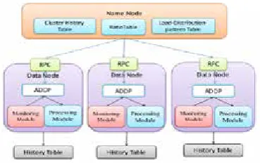
Fig. 1. Shows how the Name node deploys data blocks on data nodes

In the algorithm, there are two tables: “Ratio table” and ”Load-Distribution-Patterns table”.

Ratio table is a table that stores computing

capacity ratios of each node in different job type

and Load-Distribution-Patterns table stores load

parameters as defined average Cpu utilization

(AvgCpuUsage) and average memory utilization

(AvgMemUsage) of the whole cluster in different

load states to compare each node load parameters

with cluster load parameters. In the cluster, we assume three main states: the overloading state is defined as overload, the underloading state is defined as “underload” and the normal loading state is defined as “normalload”. There are some sub load states based on cluster load situation. These sub-states are for underload state. Every

row in table belongs to a load state .There is volume load formula for each row. Every load parameters compare with every row. If a node’s load parameters will place in any row in the

table, the formulas calculate data load volume

that is appropriate for the node’s load state to change node’s load state and make it becomes in normalload. The load volume formulas show how much workload should add to the current node’s workload to make it becomes more compatible with node’s load state so that the nodes use resources more efficient. The percentage of added workload is shown by λ factor. Next node’s volume load average (VLAi+1) is equal

to previous volume load average (VLAi) plus

a percentage of the current load average.This percentage factor is different from one row to another and depends on node load state. The percentage factors are defined in definition lambda factor table.

TABLE 1

LOAD-DISTRIBUTION-PATTERNS Load volume formula Average

Cpu Usage AverageMemory Usage load state

) (

1 1 i i i i VLA VLA

VLA+ = +λ α1≤CpuUsage≤α2 β1≤MemoryUsage≤β2 Underload

) (

2 1 i i i i VLA VLA

VLA+= +λ α2≤CpuUsage≤α3 β2≤MemoryUsage≤β3 Normal_load )

(

3

1 i i

i VLA VLA

VLA+= −λ α3≤CpuUsage≤α4 β3≤MemoryUsage≤β4 Overload

TABLE 2

DEFENITION- LAMBDA-FACTOR

Lambda

definition Load State 11

λ Very Underload

12

λ

Underload

13

λ Underload near to

Normal 2

λ

NormalLoad

21

λ

Optimize-NormalLoad

3

λ

Overload

Every load volume formula in the Load-distribution-Patterns table tries to calculate

workload that is more compatible with node load situation. So in general, we have six load levels which will be explained in the next part.

If a node state is” Very underload”, lambda

(5)

If a node state is” Underload”, lambda factor

for it in the load volume formula is ; so node’s workload which will be assigned to current node’s workload for the next round is at least 33% of node current workload plus current workload.

If a node state is” Underload near to NormalLoad”, lambda factor for it in the load

volume formula is ; so node’s workload which will be assigned to current node’s workload for

the next round is at least 20% of node current

workload plus current workload.

If a node state is” NormalLoad”, lambda

factor for it in the load volume formula is .When node’s load state is in the normal situation, most of the time there is no need to add workload to node current workload, but sometimes cluster administrator can add some more workload to the node current workload to optimize node resource utilization. In this situation the lambda factore will be and the percentage of this factor is based on administrator opinion. If a node state

is ” Overload”, lambda factor for it in the load

volume formula is ; so node’s workload which will be assigned to current node’s workload is at least 10% of node current workload minus current workload.

2. Mathematical Formulation

For making Ratio table, mathematical formulation 1 to 4 are needed and for making

Load-distribution-Patterns table mathematical formulation 5 to 8 are needed

( )

1

N

i avg

TaskExeTime i T

Number of Tasks

=

∑

(1)

avg

T ( ) (x)

NumberOfTaskSlot

t

NodeComputingCapacity=T = x ₍₂₎

t (x) t T (x) Min (x)

T

t

NodeComputingCapacityRatio R= = ₍₃₎

t

1 R (x)

( )

n t t

BlockNumber Total BlockNum

R b

x er

=

= ×

∑

(4)

( 1 1 1) ( 2 2 2)

1 2

user sys nice user sys nice

cpuUsage

Total Total

+ + − + +

=

− (5)

1 1 1 1 1 1 1 1

Total user sys nice idle IOwait irq softirq= + + + + + + ₍₆₎

2 2 2 2 2 2 2 2

Total user sys nice idle IOwait irq softirq= + + + + + + ₍₇₎

Total Memory FreeMemory Buffers Cache MemoryUsage

Total Memory

+ + +

= (8)

3. Variable Description

In the mentioned mathematical formulation, Tavg(i) denotes the average execution time to

complete a batch of tasks in the node(i) and Tt(i) shows the average time required to complete one task for the node (I) [4].

In order to get the real-time information of

CpuUsage, we can use related parameters in the file /proc/stat of Linux system to calculate CpuUsage. Seven pieces of items can be extracted from file /proc/stat: user-mode time (user),

low-priority user-mode time (nice), system mode time

(sys), idle task-mode time (idle), hard disk I/O preparing time (iowait), hardware interrupting time (irq), and software interrupting time (softirq). File /proc/stat keeps track of a variety of different statistics about the system since it was restarted. The time unit is called “Jiffy” (1/100 of Figure

axis labels are often a source of a second for×86

(6)

Journal of Advances in Computer Engineering and Technology, 2(4) 2016 22

The followings are algorithm ADDP workflow and pseudocode.

Data Input Job Input

Check if Job Type is In the Ratio Table

YES

Distribute Test DataSet and Test TaskSet

Calculate AvgCpuUsage AvgMemUsage ComputingCapacity

Ratio Is data Volume exist in

ClusterHistoy Table

Check whether Utilize Field in Cluster History Table is true

Make a record in Ratio Table and LoadDistributionPattern Table for job type

Distribute calculated Data Block Numbers on each node

Calculate each node block numbers based on Ratio Table

Calculate all nodes AvgCpuUsage AvgMemUsage

Are All Nodes AvgCpuUsage and AvgMemUsage Utilized based on LoadDistributionPattern Table

Set Utilize Fild false in Cluster history Table

NO

Set Utilize Fild True in Cluster history Table

YES

Add each node blocks number in Cluster history Table Calculate Nubmer of Distribution Data block for each Node Based on

LoadDistributionPattern Table Add Type and

Volume to ClusterHistory Table

and Type to Ratio Table

NO

Add Type and Volume to ClusterHistory Table

NO

Distribute input Data volume based on Block

Number Result in ClusterHistory Table

YES

NO

End Of Process One Job

(7)

Algorithm 1: Adaptive Dynamic Data Placement Algorithm(ADDP)

Find number of cluster’s node and number of each node’s core 1.

Find Job Type in Ratio Table 2.

IF Job Type Doesn’t exist in Ratio Table do

3.

Add Job Type and Job input Volume in Cluster-History Table and add Job Type in Ratio Table 4.

Distribute Test data and Test task on each cluster’s nodes 5.

Make a record for Job in Ratio-Table (see Algorithm(2)) 6.

Make Load- Distribution-Patterns Table (see Algorithm (3)) 7.

for each node in the cluster do 8.

Calculate BlockNumbers

9. BlockNumber= Total BlockNumber*[

∑

=

n t t

x R

1 t

) ( (x)

R _]

End

10.

for each node in the cluster do

11.

Distribute the calculated Data Block Numbers 12.

End

13.

for each node in the cluster do

14.

Calculate the AvgCpuUsage and the AvgMemUsage 15.

1

[ ]

n

x AvgCpuUsage x

NumberOfNodes

=

∑

AvgCpuUsage =

1

n

x AvgMemUsage

NumberOfNodes

=

∑

AvgMemUsage = 16.

end

17.

each node in the cluster do for

18.

Determine Node’s LoadState by comparing Node’s AvgCpuUsage and AvgMemUsage with Load- Distribution-Patterns Table

19.

Calculate Node’s new volume-load based on Node’s LoadState by using Load- Distribution-Patterns Table’s formulas.

20.

Store Node’s new volume- load in Cluster-History Table 21.

end

22.

All Node’s AvgCpuUsage and AvgMemUsage are Utilized based on Load-Distribution-Patterns Table

do If

23.

Set the Utilized flag = True 24.

Store utilized flag in utilized field in the Cluster-History Table 25.

else

26.

Set the Utilized flag = False 27.

Store utilized flag in utilized field in the Cluster-History Table 28.

end

(8)

Algorithm 1: Adaptive Dynamic Data Placement Algorithm(ADDP) (Continue)

Else

30.

Input data volume exists in Cluster-History Table do If

31.

Distribute the input Data volume based on the value of Block Numbers which exist in the Cluster-History Table

32.

Check utilized flag in utilized field in the Cluster-History Table 33.

The Input data volume is utilized based on utilized field in the Cluster-History Table do if

34.

Print “ The Cluster Is Utilized” and finish 35.

Go to 14

els e

36.

end

37.

Go to 9

Else

38.

End

39.

End

40.

41. End Of Algorithm 1

Algorithm for making Ratio-Table:

Algorithm 2: Make Ratio-Table for each node do

1.

Distribute TestTasks 2.

( )

1

N

total i

T TaskExeTime i

=

∑

Calculate Node’s TotalExeTime(Ttotal) = 3.

( ) total

avg T

T x

Number of TaskSlots =

Calculate Node’s AverageExeTime(Tavg) = 4.

Calculate Node’s ComputingCapacity (Tt) = Tavg( )x

NumberofTaskSlots

5.

Calculate Node’s ComputingCapacityRatio(Rt) =

(x)

( )

t

x t

T

Min T x

6.

end

7.

Fill Computing-Capacity-Ratio Table with (Rt) ratios 8.

Add JobType in Computing-Capacity-Ratio Table (RatioTable) 9.

End Of Algorithm 2

(9)

Algorithm for making Load-distribution-Patterns Table:

Algorithm 3: Make Load-Distribution-Patterns Table for each node in cluster do

1.

Calculate Node’s Average CpuUsage(AvgCpuUsage)

(

1 1 1

) (

2 2 2

)

1 2

user sys nice user sys nice cpuUsage

Total Total

+ + − + +

=

−

1 1 1 1 1 1 1 1

Total user sys nice idle IOwait irq softirq= + + + + + +

2 2 2 2 2 2 2 2

Total user sys nice idle IOwait irq softirq= + + + + + + 2.

Algorithm 3: Make Load-Distribution-Patterns Table (Continue)

Calculate Node’s Average MemoryUsage(AvgMemUsage)

Total Memory Free Memory Buffers Cache MemoryUsage

Total Memory

+ + + =

3.

End

4

(

)

1

( )

n

x

Calculate Cluster AverageCpuUsage LoadParameter AvgCpuUsage x NumberOfNodes

=

→

∑

5.

(

)

1 ( )

n

x

Calculate Cluster AverageMemoryUsage LoadParamete AvgMemUsage x NumberOfNodes r _→

∑

=

6.

Fill Load-distribution-Pattern Table with LoadParameters 7.

End Of Algorithm 3

(10)

When a new job is submitted to a cluster

and there is no information of that job in the

NameNode, at the first round NameNode distributes input data blocks based on values in Ratio table. In the next rounds, the whole cluster will be monitored by monitoring module.

4. Scenarios

In the monitoring phase in general, NameNode monitors each node load state and compare these

states with the values in the Load-distribution-Patterns table until node’s new workload which is more compatible with node’s load state will be calculated. For every node these calculated workloads will be registerd in the Cluster- History table and will be distributed to each node in the next rounds .

In General, based on workflow for every job which is submitted to the cluster, there are there

scenarios (three situations) described in next

subsection. The first scenario happens when a new type of job submits to cluster and there are no

information of job type and its input data volume

in the cluster. The second scenario happens when the type of job isn’t new, but its data volume is new. The third scenario happens when the type of

submitted job and its input data volume are not

new for the cluster.

4.1 Scenario 1 (Statements 1 to 16):

When a new job is submitted to a cluster and data are written into the HDFS, NameNode first checks the RatioTable. These data are used to determine whether this type of job has been performed. If there is no record of the job type in the RatioTable, It means this type of job is new and there isn’t any information of job type in the NameNode, so for distributing input data blocks, NameNode needs to make record of the job type in Ratio Table and make records of the job type and its data volume in Cluster-History Table. Then NameNode makes Load-Distribution-Patterns Table for the job type.After distributing input data blocks based on information in Ratio Table, monitoring phase will start.

4.2 Scenario 2 (Statements 18 to29):

If the RatioTable has a record of the submitted

job, it means the type of job has been performed.

Thus there is a record for the job in the

Cluster-History Table and there is

Load-Distribution-Patterns Table for the job type. Then NameNode checks job input volume in the Cluster-History table.

If the input volume of the submitted job is not on the Ratio table , it means that there is no distribution pattern for input data in the

Cluster-History table. As a result the newly written data will be allocated to each node in accordance with the computing capacity which exists in the RatioTable. After assigning input data blocks, NameNode monitors and compares each node’s load state with the values in the Load-distribution-Patterns table until the workload that is more compatible with node load situation is calculated

by load formulas in the

Load-distribution-Patterns table. This workload will register for each node in the Cluster- History table and will distribute to nodes when that job with same data input will be submitted into the cluster.

4.3 Scenario 3 (Statements 30 to 35):

If there are records of the submitted job type and its load volume input data in the Ratio table and Cluster-History table, it means that NameNode has all information for distributing input data

blocks to each node. NomeNode distributes input data blocks based on information that registered in Cluster-History table. If all nodes in the cluster are in normal load situation, the utilized field for that job with its input load volume in Cluster- History table will set True (T), otherwise will set False (F). These histories in Cluster-History table will help the NameNode to distribute input data blocks without any more effort when a job with the same workload is submitd to the cluster,

because all information for distributing input data

blocks is registered in the Cluster-History table.

IV. EXPERIMENTAL RESULT

This section presents the experimental environment and the experimental results for the

(11)

TABLE 3

EACH NODE SPECIFICATION

Machine Operating

system Memory (GB)

Number

ofCores Disk(GB)

Master Windows7 6 4 930

Slave1 Ubuntu Linux15.0 ₂ ₁ _19.8

Slave2 Ubuntu Linux15.0 ₃ ₂ _19.8

Slave3 Ubuntu Linux15.0 ₆ ₄ _583.4

A TestBed was designed for testing and comparing presented algorithm with DDP algorithm and Hadoop framework. WordCount

is a type of job runs to evaluate the performance of the proposed algorithm in a Hadoop

heterogeneous cluster. The WordCount is a

MapReduce application running on a Hadoop cluster and it is an application used for counting

the words in the input file.

The experimental environment is shown in the table. 3. We use Intel Core i5-4210U 1.70GHZ for salve1 and Intel Core i5-4210U 1.70GHZ for salve2 and Intel Core i7-4790 3.60GHZ for salve3.We use VirtualBox 4.1.14 to create our computing node for slave1 and salve2. In order to achieve the effect of a heterogeneous

environment, the capacity of the nodes is not the

same. Different amounts of CPUs and memories were set on nodes. In total, four machines were created: one master and three slaves. One machine

as the master has 4 CPUs, 6 GB of memory, and

930 GB disk; one virtual machine as a slave1 has 1 CPU, 2 GB of memory, and a 19 GB disk; one

virtual machine as a slave2 has 2 CPUs, 3GB of

memory, and a 19 GB disk; one machine as a

slave3 has 4CPUs, 6GB of memory, and a 538

GB disk.

Table 3 presents the specifications of each node. All of the slave machines adopt the operating system as Ubuntu 15.0 LTS, and the

master machine adopts the operating system as

windows 7.

TABLE 4 RATIO TABLE

Job Type Slave1 Slave2 Slave3

WordCount 1 2 4

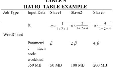
TABLE 5

RATIO TABLE EXAMPLE

Job Type Input Data Slave1 Slave2 Slave3

WordCount

α 1

1 2 4

α× + +

2 1 2 4

α ×

+ + α×1 2 4+ +4

Parametri c Each node

workload

β 2β 4β

350 MB 50 MB 100 MB 200 MB

Table 4 shows ratios for WordCount job in the RatioTable. Table 5 is made by ratios in the RatioTable and is shown if input data block is

350 MB, slave1 is assigned 50 MB, slave2 is assigned 100 MB and slave3 is assigned 200

MB. In proposed algorithm number of tasks that run on each node is based on node core numbers. Slave1 has one core, so slave1 just runs 1task in each round .Slave2 has two cores, so it runs 2 tasks in each round simultaneously. Slave3 has four cores, so it runs 4 tasks in each round simultaneously. Each job processes different input data in which the size of input data for slave

1, slave2 and slave3 are 50 MB, 100 MB and 350

MB, respectively.

Experiment 1:

In the experiment 1, a comparison is made

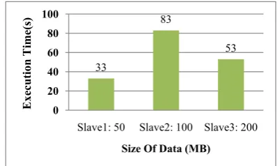
between the DDP algorithm and the ADDP algorithm when an overload state happens in the cluster. Fig 3. Shows the normal execution time of three slaves of cluster when the workloads in

normal load are 50, 100 and 200 MB for slave 1

to 3, respectively.

Slave 2 in the cluster is overloaded (Fig.4.), because it takes 240 s to finish its job (more than its normal execution time). The execution time

of WordCount is measured for each node in all rounds in DDP algorithm and ADDP algorithm

in this situation and the results is shown in Fig. 4 to Fig. 11.

The both algorithms in the first round distribute data blocks based on computing capacity ratios (Fig.4, Fig5.).

In round 2, the DDP algorithm distributes

data blocks based on computing capacity, but

the presented ADDP algorithm distributes data

blocks based on values which is registered in Cluster-History table.

(12)

this values which are calculated by Load-Distribution-Patterns table formulas. Slave2 is overloaded, so 10% of slave2 workload must be added to workload of salve3 which is underload. As a result, in round2 the nodes’ workloads

become 50MB, 90MB, 210MB and the execution times are 33s, 190s and 61s for slave1, slave2 and

slave3, respectively.(Fig.7)

The execution time 190s for slave2 is still too

much, so 10% of slave2 workload must be added to workload of salve3. As a result, in round3 the nodes’ workloads become 50MB, 81MB, 219MB

and the execution times are 33s, 141 s and 73 s for

slave1, slave2 and slave3, respectively (Fig.9).

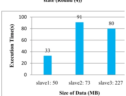
The execution time of slave2 is still too much,

so in similar approach, 10% of slave2 workload is added to workload of salve3 in round 4. Thus, in round4 the nodes’ workloads become 50MB,

73MB, 227MB and the execution times are 33s, 91s and 80s for slave1, slave2 and slave3,

respectively (Fig.11).

After four rounds the cluster with 350 MB

input data volume, is balanced and the average

execution time of the whole cluster is 68 seconds, but the average execution time of the whole cluster in DDP algorithm is 108.66 seconds.

33 83 53 0 20 40 60 80 100

Slave1: 50 Slave2: 100 Slave3: 200

Ex ecu tio n Tim e( s)

Size Of Data (MB)

Fig. 3.Execution time of each slave in normal load state

33 240 53 0 50 100 150 200 250 300

slave1: 50 slave2: 100 slave3: 200

Ex ecu tio n Tim e (s )

Fig.4.Execution time of each slave for DDP in overload state (Round (1))

33 240 53 0 50 100 150 200 250 300

Fig. 5.Execution time of each slave for ADDP in overload state (Round (1))

33 240 53 0 50 100 150 200 250 300

Fig. 6.Execution time of each slave for DDP in overload state (Round (2))

33 190 61 0 50 100 150 200

Ex ecu tio n Tim e( s)

33 240 53 0 50 100 150 200 250 300

(13)

33

141

73

0 20 40 60 80 100 120 140 160

salve1: 50 slave2: 81 slave3: 219

Ex

ecu

tio

n Tim

e

(s

)

33

240

53

0 50 100 150 200 250 300

Ex

ecu

tio

n Tim

e

(s

)

Fig. 10.Execution time of each slave for DDP in overload state (Round (4))

33

91

80

0 20 40 60 80 100

Ex

ecu

tio

n Tim

e(

s)

Size of Data (MB)

In fact, the whole cluster executions time

of the presented ADDP algorithm are reduced in each round, but executions time of the DDP

algorithm is the same in all rounds (Fig.4, Fig6, Fig8 and Fig10).

The DDP algorithm allocates data to each node

in accordance with the nodes computing capacity which is accordance to hardware, so it doesn’t work well in overload state and underload states.

In contrast, the presented ADDP algorithm not

only considers computing capacity in assigning data, but also monitors and considers load state

of nodes in assigning data block.

Experiment 2:

In the experiment 2, a comparison is made

between the DDP algorithm, the ADDP algorithm and Hadoop1.2.1 when an overload state happens in the cluster. Fig. 12 shows cluster in overload states in the Hadoop-1.2.1 framework. Fig. 13 shows execution time of the whole cluster in the Hadoop framework, the DDP algorithms and the presented ADDP when slave2 is overload. As the results shown, Hadoop framework and DDP algorithm can’t understand overloading state in the nodes and can’t handle underload

and overload state in the cluster, but ADDP can

make the corresponding adjustment to achieve

the optimal state and realize self-regulation and

decrease the execution time in each round.

80

250

83 0

100 200 300

Slave1: 116 Slave2:116 Slave3: 116

Ex

ecu

tio

n Tim

e

(s

)

Fig. 12.Execution time of each slave for Hadoop in overload state

108.66108.66108.66108.66 108.6694.66

82.33 68

137.66137.66137.66137.66

0 50 100 150

1 2 3 4

Ex

ecu

tio

n Tim

e(

s)

Execution Rounds

DDP algorithm ADDP algorithm

Fig.13.Comparison between the execution time of the whole cluster for Hadoop, DDP and ADDP algorithms,

in each round in overload state

V. CONCLUSION

This paper proposes adaptive dynamic data

(14)

algorithms classification. IN a heterogeneous environment, the difference in nodes computing

capacity may cause load imbalance and creates the necessity to spend additional overhead to

transfer unprocessed data from slow nodes to fast nodes. To improve the performance of Hadoop in heterogeneous clusters, we aim to minimize data movement between slow and fast nodes. This

goal can be achieved by a data placement scheme that distributes and stores data across multiple heterogeneous nodes based on their computing

capacities and workloads. The proposed ADDP

algorithm mechanism distributes fragments of

an input file to heterogeneous nodes based on

their computing capacities, and then calculates

each node appropriate workload base on load parameters of each node to allocate data blocks,

thereby improving data locality and reducing the additional overhead to enhance Hadoop

performance. The presented algorithm improves

the performance of Hadoop heterogeneous

clusters and significantly benefits both DataNodes and NameNode.

REFERENCE

[1] G. Turkington, 2013. Hadoop Beginner’s Guide: Packt Publishing Ltd.

[2] A. Holmes , 2012. Hadoop in practice: Manning Publications Co.

[3] R. D. Schneider, 2012. Hadoop for Dummies Special Edition, John Wiley&Sons Canada.

[4] C.-W. Lee, K.-Y. Hsieh, S.-Y. Hsieh, and H.-C. Hsiao, 2014. A dynamic data placement strategy for hadoop in heterogeneous environments, Big Data Research,1, pp. 14-22

[5] A. Hadoop, “Welcome to apache hadoop,” Hämtat från http://hadoop. apache. org, 2014.

[6] R. Xiong, J. Luo, and F. Dong, 2015. Optimizing data placement in heterogeneous Hadoop clusters, Cluster Computing, 18, pp. 1465-1480.

[7] J. Xie, S. Yin, X. Ruan, Z. Ding, Y. Tian, J. Majors, et al, 2010. Improving mapreduce performance through data placement in heterogeneous hadoop clusters, in Parallel & Distributed Processing, Workshops and Phd Forum (IPDPSW), IEEE International Symposium on, 2010, pp. 1-9.

[8] K. Singh and R. Kaur, 2014. Hadoop: addressing challenges of big data. In Advance Computing Conference (IACC), on (pp. 686-689). IEEE.

[9] X. Xu, L. Cao, and X. Wang, 2014. Adaptive task scheduling strategy based on dynamic workload adjustment for heterogeneous Hadoop clusters.

[10] P. Xu, H. Wang, and M. Tian, 2014.New Scheduling Algorithm in Hadoop Based on Resource Aware in Practical Applications of Intelligent Systems, ed: Springer, pp. 1011-1020.