Bayesian modeling for multivariate randomized incomplete block design:application in sperm biology researches

Original Article

Bayesian modeling for multivariate randomized incomplete block design: application in sperm biology researches

Abbas Rahimi Feroushani1, Mohammad Chehrazi2*, Keramat Nourijelyani1, Reza Omani Samani 3

1 _{Department of Epidemiology and Biostatistics, School of Public Health, Tehran University of Medical Sciences, Tehran, Iran} 2 _{Department of Epidemiology and Biostatistics, School of Public Health, Tehran University of Medical Sciences, Tehran, Iran}

AND Department of Epidemiology and Reproductive Health, Reproductive Epidemiology Research Center, Royan Institute, Tehran, Iran

3 _{Department of Epidemiology and Reproductive Health, Reproductive Epidemiology Research Center, Royan Institute,}

Tehran, Iran

ARTICLE INFO ABSTRACT

Received 07.04.2014 Revised 21.07.2014 Accepted 07.04.2014 Published 20.2.2015 Available online at: http://jbe.tums.ac.ir

Background & Aim: The aim of the current study was to investigate the advantages of Bayesian method in comparison to traditional methods to detect best antioxidant in Freezing of human male gametes.

Methods & Materials: Semen samples were obtained from 40 men whose sperm had normal criteria. A part of each sample was separated without antioxidant as fresh and the remaining was freezed with and without antioxidant. Taurine (in concentrations of 25 mm and50mm) and cysteine (5mm and10mm) as antioxidants were prepared as intervention. Traditional results were obtained from randomized incomplete block design and compared with Bayesian results in their ability to find the significant difference among our groups. Using Markov chain Monte Carlo algorithm within the WinBUGS software, we developed a Bayesian approach to estimate the protective effect of antioxidant against inverse effect of freezing on the quality of sperm.

Results: Classic method could detect the significant difference just in cycteine10mm for viability which was confirmed by Bayesian method. In Bayesian method, in addition to results from classic method, we could find the significant improvement in abnormality: cysteine 10mm, protamin deficiency: taurine 25 mm and10 mm, viability: cysteine 10mm, DNA fragmentation: cysteine 10mm which all of them was interested in clinically, but could not be proved by the traditional methods. Conclusion: Bayesian approach in sperm biology research can be considered as a good replacement of the traditional methods for estimation. Using this method, we can solve complex and intractable statistical models. Future researches should be done to confirm our suggestion.

Key words: Bayesian estimation, Markov chain Monte Carlo methods, cryopreservation, sperm biology, non-informative prior

Introduction1

To use statistical methods without the use of computers, if not impossible, is something very difficult. Among the many applications in analysis of data provided WinBUGS (version 1.4.3, Bayesian inferenceusing Gibbs sampling) * Corresponding Author: Mohammad Chehrazi, Postal Address:

Department of Epidemiology and Biostatistics, school of public health, Tehran University of Medical Sciences, EnghelabSquare, Pour SinaStreet, Tehran, Iran. Email: [email protected]

software is one of the most powerful and popular software used for Bayesian analysis (1). The development of Markov Chain Monte Carlo (MCMC) methods permits inference for complex models such as those, including random effects, errors in variables and hierarchical structures (2).Using MCMC, we can implement and estimate complicated models such as multivariate models that could not be solved with traditional methods easily. Biomedical researchers, usually measure several variables for outcome. Statistical methods used

for the simultaneous analysis and expression of several measured variables called multivariate analysis. Despite the correlation between outcomes even analysis is performed separately (3). Since the outcome variables are often correlated, multivariate models can be fitted to several related outcome variables. This approach can keep the alpha level closer to the nominal level and may estimate treatment effect more efficient, and may provide additional information about the relationship between variables. Turner (4) has considered multivariate models in hierarchical data and its application to cluster randomized trials. In biomedical research, many statistical methods are used in the form of various statistical designs, such as randomized complete block design (RCBD) (5). In RCBD, each treatment is given once and only once in each block. Within a block, the treatments are assigned randomly to the experimental units. Experimental unit are homogeneous in each block and this feature reduces variability that is based mainly on characteristics of the subject themselves. Occasionally, situation arise that each block does not contain a complete set of treatments, such designs are known as randomized incomplete block designs (RIBD) (6). Because the data are incomplete treatments and blocks are not orthogonal. This non-orthogonality makes that residual sum of squares would affect then poor estimates of treatment effects will produce. RIBD is stratified in mixed models class. Sammel et al. (7) has discussed about multivariate linear mixed models (MLMM) and other related models. In this paper, using MCMC algorithm, we develop a Bayesian approach to the unknown parameters in WinBUGSand apply it in real data. We provide a convenient way than traditional methods to analyze the data. The main difference between the classical statistical theory and the Bayesian approach is that the latter considers parameters as random variables that are characterized by a prior distribution. This prior distribution is combined with the traditional likelihood to obtain the posterior distribution of the parameter of interest on which the statistical inference is based. Freezing is a branch of science

cryopreservation that deals with safeguarding long cells at extremely low temperatures (8). Cryopreservation typically is carried out in infertility treatment centers and maintenance of sperm bank and industry of animal husbandry. Freezing process always reduces the capacity and yield of sperm fertility. In the past few years, the effect of different freezing methods and environment has been evaluated on sperm quality. However, the best environment for cryopreservation never has been introduced. Therefore, it seems it is essential to introduce the appropriate freezing technique and proper freezing environment based on experimental findings,whereas maintaining sperm quality andsurvival rate during the freezing process is the main objective of cryopreservation.Hence it is important for embryologists what environment with what features is better for freezing. Considering the benefits of Bayesian methods to estimate the parameters rather than classical methods (9), we decided to take this approach in the field of sperm biology and provide more accurate results for researchers in this field. We begin by describing the data which motivated our research, then formulize the model. This paper is structured as follows. Section Cryopreservation Data Base introduce data base, Section Model Formulation develops the classical and Bayesian models, Section Prior Distribution for Parameters discuss the choice and sensitivity to prior specifications. Section Results deals with some further issues and summaries the findings. Finally, discuss about models and results. The WinBUGS programs used and mathematical proofs are included in appendices A and B.

Cryopreservation Data Base

reactive oxygen and nitrogen species and oxidative stress (10). It induces membranes and nucleus alterations and also sperm DNA damage, resulting in loss of motility and decline in sperm fertilizing ability. Free radical scavenging properties of antioxidant agents may make a necessity to use them for maintaining the quality of cryopreserved semen (11). Semen samples were obtained from 40 men whose sperm had normal criteria. The samples were divided into two groups of 20. A part of each sample was separated without antioxidant as fresh and the remaining wasfreezed in three part. One part was as control without antioxidant and taurine (in concentrations of 25mm and50mm) and cysteine (5mm and10mm) as antioxidants were prepared for two another parts. Taurine to 20 samples and cysteine to other 20 samples was assigned randomly. Each group was freezed-thawed and evaluated between different concentrations and antioxidants with control and fresh. We checked the sperm quality in four criteria simultaneously including viability, DNA fragmentation, abnormal morphology and protamindeficiency. The viability of spermatozoa was assessed by the Trypan-Blue Stain method, DNA fragmentation examined by sperm chromatin dispersion test and protamin deficiency examined by Chromomycin A3. For the illustration of our methods for multivariate outcomes, we have considered this data base containing 40 blocks and 160 samples totally, which used to compare between groups and antioxidants.

Model Formulation

In this section, we introduce some notation and describe the three models that are considered, the model applied for data as RCBD (12) and we use a generalized linear mixed model (GLMM) (13). This class of models are included both continuous and discrete models and when data are measured as a continuous, usually follow normal distribution. In this paper, the responses are measured as a continuous andwe assume that are the multivariate normal distribution (3). In general model for a single outcome measured for each sample is asy , in which i indicates the level of treatment and j is block number:

y = μ + β + α + ε

ε = ~N 0, σ , α ~N 0, σ

i = 1, ich i indic

In our data base g is number of treatment levels and equal 6(fresh, control, taurine25 and50, and cysteine 5 and10) and n is number of blocks and equal 40.

where:

μereis the overall mean of response in the population of subjects and a constant

βare constants for the treatment effects,

∑ β = 0

αare independent for the block effects

ε Are independent and cov α , ε ! = 0 Let, in general, k(<g) is the number of treatment that can be applied in any block. So we define efficiency factor (EF) of the given design as EF = g k, i k g, i⁄ . EF is truly a measure of the loss in efficiency resulting from working with incomplete blocks(14). If EF is less than or equal to 0.7 perhaps with a block size of k+1 or k+2 should be considered. EF is 0.9 in our design therefore efficiency is in the acceptable range. In the balanced incomplete block design(6) the sum of square for treatment(SST) is r EF ∑ β that r define as number of block in which any treatment is applied, but obtain the SST in unbalanced type is very complicated. The intrablock correlation coefficient (ICC) is defined as ICC = σ σ ++ )_*∑ β + σ which, assuming that ICC values cannot be negative, is the correlation between measurements of individuals within blocks. Using ICC also can judge about the difference between treatment levels within each block. Different types of prior distributions and their benefits for ICC in the Bayesian models context have been discussed previously (15) recommends placing independent prior distributions on ICC and σ rather than on

covariances at both individual and block levels. Model for each outcome is as follows:

y )= μ..) + β)+ α)+ ε )

y = μ.. + β + α + ε

y .= μ... + β.+ α.+ ε .

y /= μ../ + β/+ α/+ ε /

General form response is as follows:

Y = 1Y))⋮ ⋯ Y⋱ )3⋮ Y*) ⋯ Y*3

6

ThatY = vec Y ! = y ), y , y ., y /!7. The matrix form for multivariate individual-level outcome is

Y = U + B + A + Ε (1) Where U = μ..), μ.. , μ..., μ../ 7,B =

β), β , β., β/ 7,

A = α), α , α., α/!7~MVN 0, Σ and

Ε = ε ), ε , ε ., ε /!7~MVN 0, Σ ,

cov α,, ε ,! = 0 ∀ i, j, k

Σ = A B B B

C σ ) σ ) σ ). σ )/

σ ) σ σ . σ /

σ .)

σ /)

σ .

σ /

σ _. σ /.

σ ./

σ /DE

E E F

,

Σ = A B B B

C σ , σ ,/ σ ,/ σ ,/

σ ,/ σ , σ ,/ σ ,/

σ ,/

σ ,/

σ ,/

σ ,/

σ ,

σ ,/

σ ,/

σ ,DE

E E F

where

σ _,,G = corr y _,, y _,G!Hσ _,σ _,G∀ k, kI= 1,2,3,4

andσ M,G =

corr y ,, y ,G!Hσ σ _,G∀ k, kI= 1,2,3,4

Model (1) enables us to estimate the ICC parameter. The ICC for each outcome k is defined as

ICC,= σ N+ σ N+)_*∑ β, + σ ,

We consider constraining model (1) by assuming the ICC to be identical across all three outcomes:

σ )+ σ )+)_*∑ β, + σ , =

σ _,+ σ O+)_*∑ βP + σ P ∀k, l (2)

The advantage of pooling ICC information across outcomes is that the single ICC will be estimated more precisely than the separate ICC values (4).

Regression approach

The regression approach taken to estimating the effect of treatment in Section 3 is improper for incomplete design because this model apply for complete data. If we use the routine approach for incomplete data then error variability increase and the results will be distance from truth. As mentioned in the introduction treatment and block effects are not orthogonal in incomplete block design, and so the analysis is carried out using the regression (16). One disadvantage of incomplete design is the assumption that there are no interactions between the blocking variable and the treatment is restrictive. The analysis is similar to the complete design with missing cells. We shall explain the regression approach to two-factor analysis of variance in term of two-factor effects model (2). To express this model in regression terms, we utilize indicator variables for factor treatment and factor block effects that take on the values 1, −1 or 0 as explained

below. We need a-1 indicator for the factor block effects and d-1 indicator variables for the factor treatment effects. Specifically, the regression model can be expressed in matrix notation equivalent to ANOVA model (1) for subject in jth block with ith treatment level and

kth outcome is:

Y ,=

μ..,+ Block ,⨂A ,+ treatment ,⨂B ,+

ε , (3) where for this study:

Block ,= VBlock ,) … Block ,.XY

treatment ,

= Vtreatment ,) … treatment ,ZY are indicator variables for block and treatment variable respectively.

Block ,[=

treatment ,[=

\−1 if response from treatment 6 1 if response from treatment m, for m = 1, 0 otherwise

A , and B , are regression coefficients.

Var Y ,! = Block ,Var A ,!Block ,7

+ Var ε ,

Where Var A ,! is diagonal matrix which off-diagonal elements is zero because random effects along by different level of blocks are assumed uncorrelated.

The classical multivariate analysis for regression approach have discussed by (3).Traditional analysis about multivariate (multivariate regression) done with SPSS (version 16) and has shown in table 1. Significant level for this method is 0.05. In the next section, we want to model the design in Bayesian framework. The coefficients matrix will define in the same section.

Bayesian modeling framework

We design model (3) within the Bayesian framework using MCMC simulation(2).This allows specification of prior distributions and provides a flexible framework to address complex models such as (1) and (2), which present serious difficulties for classical methods. A practical advantage of Bayesian estimation using MCMC methods is that it is straightforward to obtain interval estimates for any function of the model parameters. This enables us easily to construct

interval estimates for the ICC values, variances and for the intervention effects (15). Bayesian hierarchical models are used to estimate the effect of the intervention. Bayesian models have an inherently hierarchical structure (17) a Bayesian hierarchical model is defined when a prior distribution is also assigned on the prior parameters e associated with the likelihood parameters θ(17). Writing y ), y , y ., y /!7as the vector continuous outcomes is distributed according to multivariate normal distribution, we assume:

Y = y ), y , y ., y /!7~MVN μ , Σg !

μ = Vμ ) μ μ . μ /Y

Σg

= A B B B

C σ )+ σ ) σ ) σ ). σ )/

σ ) + σ σ . σ /

σ .)

σ /)

σ .

σ /

σ .+ σ .

σ /.

σ ./

σ /+ σ /DE

E E F

where, μ , is mean of kth response from ith treatment in jth block. Define as below:

μ ,=

μ.. ,+ block ,⨂A ,+ treatment ,⨂B ,

A ,= Vα ,) α , ⋯ α ,.XY7

B,= hβ,) β, β,. β,/ β,Zi7 The likelihood function based on the multivariate normal density function is as below:

L μ , Σ , Y !

=exp lxp l Y − μ !

7 _{Σ !}m)

Y − μ !n 2j3/ _{|Σ |}q.Z

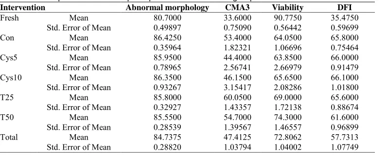
Table 1. Descriptive statistics of sperm parameter in deferent groups

Intervention Abnormal morphology CMA3 Viability DFI

Fresh Mean 80.7000 33.6000 90.7750 35.4750

Std. Error of Mean 0.49897 0.75090 0.56442 0.59699

Con Mean 86.4250 53.4000 64.0500 65.8000

Std. Error of Mean 0.35964 1.82321 1.06696 0.75464

Cys5 Mean 85.9500 44.4000 63.8500 66.0000

Std. Error of Mean 0.78965 2.56741 2.66979 0.91479

Cys10 Mean 86.3500 46.1500 65.6500 66.1000

Std. Error of Mean 0.93267 3.15417 2.08286 1.01800

T25 Mean 85.8000 60.0500 69.0000 65.6000

Std. Error of Mean 0.32927 1.43357 1.72138 0.88674

T50 Mean 85.5500 54.7000 74.3000 61.6000

Std. Error of Mean 0.28539 1.39567 1.46557 0.96899

Total Mean 84.7375 47.4125 72.8062 57.7313

where, μ is a vector with fourelements including mean responses for subject in jth block with ith treatment level, and Σ is variance-covariance matrix with dimension 4 is for responses in jth block and ith treatments. The parameters A , and B , reflect the coefficient matrix for the block and treatment respectively. For a better understanding of notations and symbols, we define multivariate modeling at individual-level outcome. However, all of them have coded to multivariate mode in software. The above model can be fitted using SPSS software in a non-Bayesian fashion. A Bayesian analysis requires, in addition, prior specification for all unknown parameters in the model. The posterior density function for the model parameters is proportional to the product of the likelihood function and the prior density of all the model parameters. This posterior is computed automatically by WinBUGS, so in here no need to calculate it.

Prior Distribution for Parameters

As vague prior distributions for the regression coefficients for each treatment and block level, we choose the multivariate normal distribution. The Wishartdistribution (3) is a standard choice of non-informative prior for a covariance matrix, and this would be a possible prior distribution for each of Σ and Σ . We should specify separate priors for different elements within

σ and Σ because it is not possible to incorporate prior information on the ICC when using Wishart distributions. When selecting prior distributions for the variance parameters in the case of four multivariate outcomes, it must be ensured that the matrix formed by each set of elements is nonnegative definite and thus valid as a covariance matrix. In the context of multivariate (18), declared prior distributions for variance and correlation parameters in the bivariate case, but acknowledged the difficulty of doing this in the case of three or more outcomes, without proposing a solution. We develop a solution by considering the Choleskydecomposition (19), which ensures that a symmetric matrix is non-negative definite if and only if there exists an upper triangular

matrix C such that Σ9C7_{C and C is unique.The} derivation of the Cholesky decomposition for covariance matrix and the WinBUGS programs used are included in appendix B. Σ is variance-covariance matrices for regression coefficients in each level of treatment effects, where:

Σr=

A B B B

C σr σr s σr s σr s

σr s σr σr s σr s

σr s

σr s

σr s

σr s

σ_r σr s

σr s

σ_{r D}E E E F

The prior distribution for elements within the covariance matrices is gamma as non-informative; In particular we use the priors given by:

β), β , β., β/ 7~MVN 0, Σr

α), α , α., α/!7~MVN 0, Σ

where Σr,Σ and Σ are positive definite matrices,

σ t~Γ 0.001,0.001 , k = 1,2,3,4

σ _,~Γ 0.001,0.001 , k = 1,2,3,4

σr ~Γ 0.001,0.001 , k = 1,2,3,4

icc~beta 0.001,0.001

corr y ,, y ,G!~u 0,1

In our work, we use some priors that (15) has investigated like log-uniform, uniform for σ w,

σ , and uniform shrinkage for ICC and result will be compared.

Log-uniform distribution for x_yz{ , x_|}{

In this case, we assume a log-uniform distribution for σ ~ andσ , on a bounded range (emt,et), thus

f σ _,! = 1 2aσ⁄ _, exp −a < σ_r,< €•‚ ƒ f σ _,! = 1 2aσ⁄ _, exp −a < σ _, < €•‚ ƒ

Which ICC prior distribution is as follow (all formulas in this section are proven in appendix A),

f icc = 2a − logiticc Vicc 1 − icc 4a Y⁄ , 0 < icc < exp 2a 1 + exp 2a⁄

Table 2 shows the result of this prior for arbitrarily chosen value a=5.

Uniform distribution for x_y}{ ,x_|}{

According to opinion Gelman et al. (20) a uniform prior distribution considered for variance matrix component, so there:

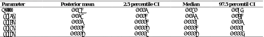
Table 2. Posterior estimates for ICC and correlation between four outcomes in full model

Parameter Posterior mean 2.5 percentile CI Median 97.5 percentil CI

Corr 0.033 0.001 0.028 0.095

Icc[1] 0.013 0.006 0.012 0.026

Icc[2] 0.001 0.0006 0.001 0.001

Icc[3] 0.0006 0.0004 0.0006 0.001

Icc[4] 0.0005 0.0003 0.0004 0.0007

In this model σ and σ„ have beta distribution with non-informative hyperparameters ICC: Intrablock correlation coefficient; CI: Credible interval

Table 3. Posterior estimates for ICC and correlation between four outcomes I the multivariate model

Parameter Posterior mean 2.5 percentile CI Median 97.5 percentil CI

Corr 0.035 0.001 0.030 0.097

Icc[1] 0.013 0.006 0.011 0.026

Icc[2] 0.001 0.0006 0.0009 0.001

Icc[3] 0.0006 0.0004 0.0006 0.0009

Icc[4] 0.0004 0.0003 0.0004 0.0007

In this model σ and σ„ have Log-uniform distribution with non-informative hyperparameters ICC: Intrablock correlation coefficient; CI: Credible interval

f σ _,! = 1 a⁄ 0 < σ _,< ƒ

Where, the prior distribution is as follow:

f icc = …1 2icc_{1 2 1 − icc}⁄_⁄ icc > 0.5 _{icc ≤ 0.5}

In this case, WinBUGS program was run for arbitrarily value 10 for a and the result are listed in table 3. Then, we let prior distributions such as Uniform-Shrinkage and truncated normal for the parameter ICC.

Uniform-shrinkage

Daniels (21) and Natarajan and Kass (22) suggested a uniform prior on the shrinkage parameter v = 1 − icc V1 + k − 1 iccY⁄ for producing robust estimators with good sampling properties. In appendix A, we show that the prior density function for ICC is as below:

f icc = k 1 + k − 1 icc⁄ 0 < icc < 1

where a log-uniform (−a,a) prior let for σ _,,

the marginal distribution for σ , can be obtained through mathematical statistics relationships (Appendix A).

The analyses described above cannot be carried out in closed form, and even analytic approximations can be difficult (23). Bayesian analysis has made extensive use of MCMC methods, in which sensible values for the parameters are simulated from their joint posterior distribution.

The MCMC algorithm used within the

WinBUGS software is Gibbs sampling (17). Version of the software used is 3.0.2 (1).The algorithm was run for 43,500 iterations which discarding the initial 3500 iterations as burn-in. The posterior means and 95% credible intervals for parameters are shown in table 4. For test of treatment effect, we use credible interval for interpret each coefficient and also deviance information criterion (DIC) (24), Bayesian information criterion (BIC), and Akaikeinformation criterion (AIC) for overall effect. Latter criterions use for measure the goodness of fit of an estimated statistical model. Low values of these indicate better-fitted models (17). Their formulas are as follows:

DIC = pŠ+ D‹

pŠ= D‹ − DŒ

D θ = −2 log f y|θ)!

where, pŠ is the penalty for over-parameterizing the model and θ are the unknown parameters of the model and f(y|θ) is the likelihood function.

D‹ = Expectation D(θ)!

DŒ = −2log (f(y|θ•))

θ•is the posterior mean of stochastic nodes. This criterion is particularly useful in Bayesianmodel selection problems where the posterior distributions of the models have been obtained by MCMC simulation (24).

BIC = DΠ+ 2Plog(n)

Table 4. Posterior estimates for the regression coefficient from the multivariate model

Groups Effects of antioxidant 2.5 percentile CI 97.5 percentile CI Overall mean

Fresh -4.419 -5.961 -2.862

85.33

Control 1.303 -0.2492 2.853

Cys 5 0.5894 -1.594 2.787

Abnormal morphology Cys 10 0.3383 -1.851 2.567

T 25 0.8964 -1.31 3.109

T 50 1.291 -0.9384 3.512

Fresh -15.1 -16.67 -13.57 48.51

Control 4.688 3.112 6.227

Cys 5 9.279 7.072 11.5

Protamin Deficiency Cys 10 3.935 1.717 6.141

T 25 -2.279 -4.522 -0.07297

T 50 -0.5202 -2.76 1.689

Fresh 19.49 17.94 21.05 71.32

Control -7.215 -8.754 -5.666

Cys 5 -2.196 -4.391 -0.02061

Viability Cys 10 3.092 0.9013 5.264

T 25 -7.487 -9.679 -5.32

T 50 -5.688 -7.86 -3.502

Fresh -24.6 -26.15 -23.04 59.61

Control 5.711 4.147 7.279

Cys 5 5.802 3.608 7.982

DNA Fragmentation Cys 10 1.801 -0.3862 4.017

T 25 5.592 3.42 7.783

T 50 5.693 3.499 7.892

CI: Credible interval; Fresh: Fresh group; T 25: Taurine 25 group; T50: Taurine 50 group; Cys5: Cysteine 5 group Cys10: Cysteine 10 group; Control: Control group

where, P is number of parameters and n is number of observations.

The value of ICC estimate correlation between treatment levels in each block. Traditional analysis (multivariate analysis of variance) done with SPSS (version 16) and has come in the result part. Significant level for this method is 0.05.

Results

In this article, results are divided into two parts for better comparison, classic and Bayesian. Classic method could detect the significant difference between control and case in the following group which was confirmed by Bayesian method.

Relative to the control group supplement with cysteine (10 mm) improved post-thaw viability. Mean difference is significant at level 0.05 (P < 0.0001). DNA fragmentation: cysteine 10mm supplementation decreased this outcome and mean difference with control group was significant (P < 0.0001). In morphology and protamin deficiency none of antioxidants show any significant effect. All of ANOVA results

have been shown in table 1. In Bayesian method we could find significant improvement in some outcomes. DIC, BIC, and AIC criteria is given in table 3 which compare full and reduce models. We use the credible intervals for significant individual regression coefficients in Bayesian method, the results for each response is as follows:

As you can see in table 4, overall mean for abnormal morphology has obtained 85.33. Effect of Fresh group on this response is −4.41, which

shows the abnormality in this group being less than the control group. Effect of cysteine 10 on abnormality is 0.33, which represent more effective than dosage 5. The effect of taurinein a dose of 25 and 50 are 0.89 and 1.29, respectively. Other outcomes are interpreted as the same. Overall mean in the second outcome protamine deficiency is 48.51. Considering the effect of fresh group on this response, the protamine deficiency average is less than the total population for this group. Effect of the control group is 4.68 showing deterioration of sperm quality in freezing mode. Between treatment groups, taurinewith dose 25 and 50 indicate better action than other groups including control, and reduces the effect of freezing on the response. In the third response, viability, as you can see in the control group the effect of freezing on viability is significant. Negative effect for this group has caused the average of viability become less than overall mean whereas antioxidant cysteine 10 has improved viability compared withcontrol group because of this antioxidant effect (3.092) against freezing is positive. Finally, in the fourth response DNA fragmentation the effect of control group show large influence of freezing on DNA fragmentation and therefore destruction was increased. Among the antioxidant groups, although there is still increasing in DNA fragmentation but the effect of antioxidant cysteine 10 is better than others and freezing makes that DNA fragmentation not increase much. All of improvement was expected clinically. Table 2 contains the correlation coefficient between responses and ICC that is correlation between levels of treatment effect.

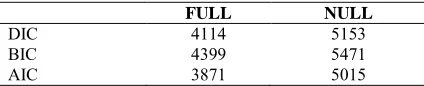
ICC values for all four variables is close to zero, which indicates difference in the effects of levels on the response because, if the ICC values be high therefore the effect of levels are close to each other. Tables 3 and 5 show same quantities for various distribution of σ and σ which results are similar to table 2. However, in table 6, a joint ICC is obtained through shrinkage parameter, which the value is higher than the previous case. ICC can be more for this reason that some treatment levels have no significant differences and therefore its value has led to 1. As we mentioned in previously joint ICC is more accurate than individual, which is obvious here. As shown in table 7, three criterions have been presented for comparing models which all of them were calculated in both full and reduced. However, these criteria are less so the model is better. Here, three criterions know full model with treatment is better. Figure 1 shows the posterior density plots for the effects of treatment. As you can see all of them have converged to the normal distribution by Gibbs algorithm. Figure 2 to 5 present posterior density plots for ICC in various σ and σ distributions.

Discussion

One problem with the model discussed by (7) was that overall mean for the effect of treatment cannot estimate but in the regression model using the Bayesian perspective is estimable. The model were presented in this paper is an extension of the approaches of (4) for incomplete randomized block design. There is variation between blocks within each block that makes it a correlation is formed.

Table 5. Posterior estimates for ICC

Parameter Mean 2.5 Median 7.5

Icc[1] 0.013 0.006 0.012 0.027

Icc[2] 0.001 0.0007 0.001 0.001

Icc[3] 0.0007 0.0004 0.0006 0.001

Icc[4] 0.0005 0.0003 0.0005 0.0007

In this model σ and σ„ have uniform distribution with non-informative hyperparameters ICC: Intrablock correlation coefficient

Table 6. The joint ICC for multivariate model.

Parameter Posterior mean 2.5 percentile CI Median 97.5 percentil CI joint ICC 0.2817 0.006212 0.1987 0.9078

Table 7. Diagnostic criterion for compare full and null

model

FULL NULL

DIC 4114 5153

BIC 4399 5471

AIC 3871 5015

DIC: Deviance information criterion; BIC: Bayesian information criterion; AIC: Akaikeinformation criterion

Acquire this correlation in classical method is very complex, however, in Bayesian methods such calculations are carried out easily. The main advantage of the proposed methods is that prior information on the intra-class correlation coefficient can be included in the analysis. In the traditional methods, estimating ICC in multivariate mode is very complex and intolerance. Another advantage of the model described here is that we can obtain direct estimates of factors effect, which make the analysis much easier to interpret and more plausible, while the estimate of this parameter is not customary in the traditional analysis. At incomplete designs estimate of parameters is affected by missing data therefore, wrong inference will come from the wrong results. The missing could be estimates by simulation methods like MCMC easily with acceptable accuracy. In Bayesian methods reflect investigators’ prior belief about the strength of the investigated association as well as the quality of instruments to be used in exposure assessment. Such knowledge formally incorporates into quantitative rather than qualitative appraisal of the data. Both Bayesians and frequentists alike have problems to rely on prior information in many trials including clinical and experimental. However, only Bayesians bind themselves to formally participate it in analysis. The prior information in Bayesians directly affects the estimate, while in frequentists does not. There are many ways at Bayesian disposal to provide that the faulty prior information do not enroll in analyses, such as the use of vague, non-informative priors.

The present methodology deals with a single factor. There are interesting issues surrounding extensions to multiple factors or combinations of factors plus covariates. This methodology, plus suitable extensions to incorporate the features

mentioned should be widely applicable in the block design and other design too.

However, results of a Bayesian analysis are sensitive to prior assumptions; we note that apparently non- informative priors can be strongly influential.

Earlier using Bayesian perspective was discussed by (4) in the multivariate Cluster Randomized Trials however, about block designs little effort has been taken in the field of Bayesian. Future research in this area will be required to adapt the methods presented in this paper to deal with other types of outcome data such as binary, count, nominal and ordinal data and other multivariate design such as repeated measurement, Latin square, split plot and so on. There is still considerable work needed in establishing robust strategies for Bayesian modeling that will provide convincing and generally acceptable results. In the meantime, we would recommend using background knowledge to produce an informative prior on the ICC where appropriate.

Conclusion

Bayesian is a well-qualified statistical approach in sperm biology research and can be considered as a good replacement of the traditional methods like analysis of variance. Using this method we can solve complex and intractable statistical models. Future researches should be done to confirm our suggestion.

Acknowledgments

We thank Royan Institute and Tehran University of Medical Sciences which helped to improve this paper. We thank Embryology department for permission to use data from the trial.

References

1. Spiegelhalter D, Thomas A, Best N, Lunn D. WinBUGS user manual [Online]. [cited 2003 Jan]; Available from: URL:

http://www.politicalbubbles.org/bayes_beach /manual14.pdf

learning. Machine LearningJanuary 2003; 50(1-2): 5-43.

3. Anderson TW. An introduction to multivariate statistical analysis. 3rd _ed.

Hoboken, NJ: John Wiley & Sons; 2003. 4. Turner RM, Omar RZ, Thompson SG.

Modelling multivariate outcomes in hierarchical data, with application to cluster randomised trials. Biom J 2006; 48(3): 333-45. 5. Fleiss JL. Design and analysis of clinical experiments. 1st _{ed. Hoboken, NJ: Wiley;}

1999.

6. Yates F. Incomplete randomised blocks. Annals of Eugenics 1936; 7(2): 121-40. 7. Sammel M, Lin X, Ryan L. Multivariate

linear mixed models for multiple outcomes. Stat Med 1999; 18(17-18): 2479-92.

8. Mortimer D. Practical laboratory andrology. Oxford, UK: Oxford University Press; 1994. p. 301-23.

9. O'Hagan A. Bayesian statistics: principles and benefits. Wageningen UR Frontis Series 2004; 3: 32-45.

10. Chatterjee S, Gagnon C. Production of reactive oxygen species by spermatozoa undergoing cooling, freezing, and thawing. Mol Reprod Dev 2001; 59(4): 451-8.

11. Parks JE, Graham JK. Effects of cryopreservation procedures on sperm membranes. Theriogenology 1992; 38(2): 209-22.

12. Quinn GP, Keough MJ. Experimental design and data analysis for biologists. 1st _ed.

Cambridge, UK: Cambridge University Press; 2002.

13. West BT, Welch KB, Galecki AT. Linear mixed models: A practical guide using statistical software. New York, NY: CRC

Press; 2006.

14. Fleiss JL. Balanced incomplete block designs for inter-rater reliability studies. Applied Psychological Measurement 1981; 5: 105-12. 15. Spiegelhalter DJ. Bayesian methods for

cluster randomized trials with continuous responses. Stat Med 2001; 20(3): 435-52. 16. Kutner MH, Neter J, Nachtsheim CJ, Li W.

Applied linear statistical models. 5th ed. New York, NY: McGraw-Hill Education; 2005. 17. Ntzoufras I. Bayesian modeling using

WinBUGS. Hoboken, NJ: Wiley; 2009. 18. Nam IS, Mengersen K, Garthwaite P.

Multivariate meta-analysis. Stat Med 2003; 22(14): 2309-33.

19. Tanabe K, Sagae M. An exact cholesky decomposition and the generalized inverse of the variance-covariance matrix of the multinomial distribution, with applications. Journal of the Royal Statistical Society, Series B 1992; 54(1): 211-9.

20. Gelman A, Carlin JB, Stern HS, Rubin DB. Bayesian Data Analysis. New York, NY: Chapman & Hall/CRC; 1995.

21. Daniels MJ. A prior for the variance in hierarchical models. The Canadian Journal of Statistics 1999; 27(3): 567-78.

22. Natarajan R, Kass RE. Reference bayesian methods for generalized linear mixed models. J Amer Statist Assoc 2000; 95(449): 227-37. 23. Harville DA. Maximum likelihood

approaches to variance component estimation and to related problems. J Amer Statist Assoc 1977; 72(358): 320-38.

Appendix A

Cholesky decomposition assume that a symmetric matrix Σ is non-negative definite matrix when there is an upper triangular matrix C such thatΣ = C7⨂C. Let A is a vector of independent standard normal variables, where Y=C⨂A. The elements of Y will each have unit variance with the matrixΣ, the component of matrix C is as follows:

Σ = •

s)) s)

s ) s

s).

s .

s)/

s /

s.) s. s_.. s_./

s/) s/ s_/. s_//

• =

•

a)) 0

a) a

0 0 00 a). a . a.. 0

a)/ a / a./ a//

• •

a)) a)

0 a aa)..

a)/

a /

0 0 a.. a./

0 0 0 a/

•

where elements of matrix C can be written based on Σ matrix elements. Through this component matrix C can be obtaind:

a))= √s))

a) = s) ⁄√s11

a).= s).⁄√s))

a)/= s)/⁄√s))

a = Hs −s’““

s’’

a .= s .− s).s) ⁄s)) +Hs −s_s’““_’’

a /= s /− s)/s) ⁄s)) Hs −s’“

“

s’’

+

a..=

”s..−s’•

“

s’’− – s .− s).s) ⁄s)) Hs −

s’““

s’’

+ —

a./=

s•˜ms’•s’˜⁄s’’m

™ š

›_{œ“••œ’“œ’• œ’’}⁄

”œ““•œ’“_œ’’“ _žŸ

™ š

›_{œ“˜•œ’“œ’˜ œ’’}⁄

”œ““•œ’“_œ’’“ _žŸ

¡s••mœ’•_œ’’“ m¢ s“•ms’•s’“⁄s’’£”s““mœ’“_œ’’“ ¤ “

a//=

s//−s’˜

“

s’’− – s /− s) s)/⁄s)) Hs −

s_’““

s’’ + — − ™ š š š š š š š š š š š

›s•˜ms’•s’˜⁄s’’m

™ š

›_{œ“••œ’•œ’“ œ’’}⁄

”œ““•œ’“_œ’’“ _žŸ

™ š

›_{œ“˜•œ’˜œ’“ œ’’}⁄ ”œ““•œ’“_œ’’“ _žŸ

¥ ¦¦ ¦¦ ¦¦ ¦¦ ¦§

s••mœ’•_œ’’“m

™ š

›_{œ“••œ’•œ’“ œ’’}⁄

”œ““•œ’“_œ’’“ _žŸ “ ž Ÿ Ÿ Ÿ Ÿ Ÿ Ÿ Ÿ Ÿ Ÿ Ÿ Ÿ

Mathematical solutions for different prior density functions are as follows:

Suppose X and Y have independent gamma (a,b) then probability density function for

Z = X X + Y⁄ obtain as follows:

ªZ = X X + Y_{U = X + Y}⁄ -®®®®¯ ª X = ZU3« ¬s _{Y = U − ZU} ,

J = ± U_{−U 1 − Z± = U}Z f²,³ z, u =~

µ¶· _¸~¹•’_º“¹ ¶ ’•µ_{V~ )m¸ Y}¹•’

» t » t

Integrating out U reveals a marginal distribution

f² z =_{¼ t,t}) ztm) 1 − z tm) ,0 < Z < 1 whereB a, b =» t » º_{» t½º} and Z has beta distribution.

Let V = LnX and U = LnY are independent identically distributed as Uniform a, b with density f¾ v = f³ u =_ºmt) , then X and Y have Log-Uniform distribution:

f¿ x =_{x b − a e}1 t < À < eº

fg y =_{y b − a e}1 t < Á < eº

Now, we can obtain density function for z =_¿½g¿

Jacobean for variables Z and U = X + Y is U. The joint distribution for Z and U is then

f³,² u, z = u_{¸~ ºmt}) _{V~ )m¸ Y ºmt})

f² z = _{¸ )m¸ ºmt}ºmt mPw* 7 ¸“ ,0 < Z < ·

)½ ·

Suppose X and Y are independent Uniform distributed with limited ranges (0, a) and (0, b) respectively. We change this variables to

z =_¿½g¿ and U = X + Y and Jacobean is U. The marginal distribution for Z obtain as bellow:

f²,³ z, u =_tº~

f icc = Â

t

º¸“ icc > 0.5

º

t )m¸“ icc ≤ 0.5

Appendix B

Applied WinBUGS codes are as follows: model{

for(j in 1:b){

y[j,1:c] ~ dmnorm(mu[,j] , T[j,1,,]) y.pred[j,1:c]~dmnorm(mu0[,j] , T0[j,1,,]) }

for(k in 1:c){ for(j in 1:b){ x[1,k,j,1]<-1

x[1,k,j,2]<-equals(treat1[j,k] , 1) - equals(treat1[j,k], 2)

for(h in 3:6){

x[1,k,j,h]<-equals(treat1[j,k] , h) - equals(treat1[j,k] , 2)

}

for(l in 7:45){

x[1,k,j,l]<-equals(block1[j,k],l-6) - equals(block1[j,k] , 40)

}

mu[k,j]<- inprod(x[1,k,j,1:6] , beta[1:6,k]) + inprod(x[1,k,j,7:45] , alpha[1:39,k]) yi.lower.pred[j,k]<-step(y.pred[j,k]-y[j,k]) F.pred[j,k]<-sum(yi.lower.pred[1:j,k])/b }}

### priors for(k in 1:c){

beta[7,k]<- -sum(beta[2:6,k]) alpha[40,k]<- -sum(alpha[1:39,k]) }

for(u in 1:6){

beta[u,1:c] ~ dmnorm(mu2[] ,T2[,]) }

for(v in 1:39){

alpha[v,1:c] ~ dmnorm(mu2[] , T3[,])

}

for(k in 1:c){ icc[k]<-

tau.a/(tau.a+(1/6)*(inprod(beta[2:7,k],beta[2:7,k ]))+tau.e)

}

tau.e ~ dgamma(0.001,0.001) corr1~dunif(0,1)

for(j in 1:b){ A[j,1,2,1]<-0 A[j,1,3,1]<-0 A[j,1,3,2]<-0 A[j,1,4,1]<-0 A[j,1,4,2]<-0 A[j,1,4,3]<-0

A[j,1,1,1]<-sqrt(tau.e)

A[j,1,1,2]<-(corr1*tau.e)/A[j,1,1,1] A[j,1,1,3]<-(corr1*tau.e)/A[j,1,1,1] A[j,1,1,4]<-(corr1*tau.e)/A[j,1,1,1] A[j,1,2,2]<-sqrt(tau.e- pow(A[j,1,1,2],2))

A[j,1,2,3]<-((corr1*tau.e)-(A[j,1,1,2]*A[j,1,1,3]))/A[j,1,2,2] A[j,1,2,4]<-((corr1*tau.e)-(A[j,1,1,2]*A[j,1,1,4]))/A[j,1,2,2]

A[j,1,3,3]<-sqrt(tau.e-pow(A[j,1,2,3],2)-pow(A[j,1,1,3],2))

A[j,1,3,4]<-((corr1*tau.e)-

(A[j,1,1,3]*A[j,1,1,4])-(A[j,1,2,3]*A[j,1,2,4]))/A[j,1,3,3]

A[j,1,4,4]<-sqrt(tau.e - pow(A[j,1,1,4],2) - pow(A[j,1,2,4],2) - pow(A[j,1,3,4],2))

for(n in 1:4){ for(m in 1:4){

T[j,1,n,m]<-((1-equals(n,m))*corr1*tau.e)+equals(n,m)*tau.e }}

}

tau.a~dgamma(0.001,0.001) corr2~dunif(0,1)

##Cholesky decomposition for T3 D[2,1]<-0

D[3,1]<-0 D[3,2]<-0 D[4,1]<-0 D[4,2]<-0 D[4,3]<-0

D[1,1]<-sqrt(tau.a)

D[1,4]<-(corr2*tau.a)/D[1,1] D[2,2]<-sqrt(tau.a - pow(D[1,2],2))

D[2,3]<-((corr2*tau.a)-(D[1,2]*D[1,3]))/D[2,2] D[2,4]<-((corr2*tau.a)-(D[1,2]*D[1,4]))/D[2,2]

D[3,3]<-sqrt(tau.a-pow(D[1,3],2)-pow(D[2,3],2))

D[3,4]<-((corr2*tau.a)-(D[1,3]*D[1,4])-(D[2,3]*D[2,4]))/D[3,3]

D[4,4]<-sqrt(tau.a - pow(D[1,4],2) - pow(D[2,4],2) - pow(D[3,4],2))

for(n in 1:4){ for(m in 1:4){

T3[n,m]<-((1-equals(n,m))*corr2*tau.a)+equals(n,m)*tau.a }}

tau.b~dgamma(0.001,0.001) corr3~dunif(0,1)

##Cholesky decomposition for T2 M[2,1]<-0

M[3,1]<-0 M[3,2]<-0

M[4,1]<-0

M[4,2]<-0 M[4,3]<-0 M[1,1]<-sqrt(tau.b)

M[1,2]<-(corr3*tau.b)/M[1,1] M[1,3]<-(corr3*tau.b)/M[1,1] M[1,4]<-(corr3*tau.b)/M[1,1] M[2,2]<-sqrt(tau.b - pow(M[1,2],2))

M[2,3]<-((corr3*tau.b)-(M[1,2]*M[1,3]))/M[2,2] M[2,4]<-((corr3*tau.b)-(M[1,2]*M[1,4]))/M[2,2]

M[3,3]<-sqrt(tau.b-pow(M[1,3],2)-pow(M[2,3],2))

M[3,4]<-((corr3*tau.b)-(M[1,3]*M[1,4])-(M[2,3]*M[2,4]))/M[3,3]

M[4,4]<-sqrt(tau.b - pow(M[1,4],2) - pow(M[2,4],2) - pow(M[3,4],2))

for(n in 1:4){ for(m in 1:4){

T2[n,m]<-((1-equals(n,m))*corr3*tau.b)+equals(n,m)*tau.b }}