Journal of Computing and Security
New Functions for Mass Calculation in Gravitational Search
Algorithm
Sepehr Ebrahimi Mood
a,∗
, Esmat Rashedi
b, Mohammad Masoud Javidi
a aDepartment of Computer Science, Shahid Bahonar University of Kerman, Kerman, Iran.bDepartment of Electrical Engineering, Graduate University of Advanced Technology, Kerman, Iran.
A R T I C L E I N F O.
Article history: Received:18 May 2015
Revised:04 June 2016
Accepted:27 August 2016
Published Online:30 September 2016
Keywords:
Gravitational Search Algorithm, Heuristic Search Algorithm, Scaling Functions, Exploration and Exploitation, Mass Calculation.
A B S T R A C T
Nowadays, optimization problems are large-scale and complicated, so heuristic optimization algorithms have become common for solving them. Gravitational Search Algorithm (GSA) is one of the heuristic algorithms for solving optimization problems inspired by Newton’s lows of gravity and motion. Definition and calculation of masses in GSA have an impact on the performance of the algorithm. Defining appropriate functions for mass calculation improves the exploitation and exploration power of the algorithm and prevents the algorithm from getting trapped in local optima. In this paper, Sigma scaling and Boltzmann selection functions are examined for mass calculation in GSA. The proposed functions are evaluated on some standard test functions including unimodal functions and multimodal functions. The obtained results are compared with the standard GSA, genetic algorithm, particle swarm optimization algorithm, gravitational particle swarm algorithm and clustered-GSA. Experimental results show that the proposed method outperforms the state-of-the-art optimization algorithms, despite the simplicity of implementation.
c
2015 JComSec. All rights reserved.
1
Introduction
Heuristic search algorithms and swarm intelligence algorithms are techniques used to solve large and com-plicated problems for which the classical methods are too slow or not successful. Nowadays, in many kinds of real-world optimization problems, such as robotics [1–3] , networking [4] , economy [5] , medicine [6–8] , modern physics [9] , art and fashion design [10] , se-cure communication [11] , filter modeling [12] , indus-trial problems [13–16] , and image processing [17, 18] ,
∗ Corresponding author.
Email addresses:sepehr [email protected](S. Ebrahimi Mood),[email protected](E. Rashedi),
[email protected](M. M. Javidi)
ISSN: 2322-4460 c2015 JComSec. All rights reserved.
heuristic random search algorithms are used. The use of natural laws in swarm intelligence and optimiza-tion algorithms is very common. The Gravitaoptimiza-tional Search Algorithm (GSA) [19] is one of the heuristic al-gorithms that has been inspired by Newtonian’s laws of motion, gravity, and mass interactions. Experimen-tal results indicate that this algorithm has performed very well in solving different kinds of optimization problems and is also simple to implement [19, 20].
forces.
Up to now, efforts have been made to improve the performance and efficiency of the GSA and the re-sults have been very impressive. Some researchers have proposed other versions of this algorithm, such as the quantum gravitational search algorithm (QGSA) which has fast convergence speed [21] . Furthermore, some works added new operators to the computational process of the algorithm, like the “black hole” inspired by astronomical phenomenon which is used to improve the exploitation [22] or “disruption” originating from astrophysics that improves the ability of GSA to fur-ther exploit and explore the search space [23] . Saeidi and Rashedi [24] controlled the parameters of GSA by a fuzzy controller to balance between the powers of ex-ploitation and exploration and get better results with fewer iterations of the algorithm. Clustered GSA [25] is used to reduce the computations in GSA. Some of the important ideas and research in GSA are reviewed in [26].
Scaling functions could be applied for mass calcula-tion in the computacalcula-tional process of GSA to balance the exploitation and exploration of the algorithm. At the beginning of the algorithm, due to the large stan-dard deviation of objective function values, it is better for the masses of objects to be close to each other to have a higher exploration power. But, as getting closer to the end of the algorithm, a higher exploita-tion power is needed to reach the best answer. This aim can be achieved by increasing the differences be-tween the masses of the objects, thus having stronger gravitational forces from heavier objects to the other objects. In this paper, Boltzmann and Sigma scaling functions are used for mass calculation in GSA.
The remainder of this paper is organized as follows. Section 2 introduces the principles of the gravitational search algorithm. In Section 3, the proposed function for mass calculation in gravitational search algorithm is presented and the needs of this method in detail are discussed. Assessment and review of the experimen-tal results are presented in Section 4 and finally, in Section 5 a brief conclusion is presented.
2
Gravitational Search Algorithm
Gravitational search algorithm, GSA, is a novel heuris-tic algorithm which obeys the law of gravity and sim-ulates Newton’s gravitational force and motion be-haviors to optimize a single objective. Experimental results show that this algorithm in addition to the sim-plicity of implementation has a proper performance in solving different kinds of optimization problems [19, 20].
In GSA, agents are a collection of objects whose weights depend on their performance. All these objects are attracted to each other by gravitational force. By these forces, they can transmit the information about the search space.
In a system withN objects (agents), the position ofithobject fori= 1, ..., N is denoted by:
Xi = (x1i, ..., xid, ..., xmi ), i= 1, ..., N (1)
where xdi is the position of ith agent in the dth
dimension andmis the search space dimension. The amount of force acting on objecti from objectj at timetis calculated as follows:
Fijt = Maj×Mpi
Rij(t)rP ower+ε
(xdj(t)−Xid(t)) (2)
Maj is the active gravitational mass ofithobject,
Mpiis the passive gravitational mass ofithobject and
G(t) is the gravitational constant in time t. In this paper, the value ofrP oweris considered to be 1. ε
is a small value andRij(t) is the Euclidean distance
between objectsiandjwhich is computed as follows:
Rij(t) =kXi(t), Xj(t)k2 (3)
To create a randomness property in GSA, the total forceFid that acts onithobject in thedthdimension is equal to the sum of weighted random forces from
dth component of other objects. We can compute this force using Equation (4). Kbest is the set of K heavier objects in which K is a function of time, initialized toK0 at the beginning of algorithm and
linearly decreased with time.
Fid= X
j∈Kbest,j6=i
randjFijd(t) (4)
Where randj is a uniformly distributed random
number in the interval [0 , 1].
According to the law of motion, the acceleration of objectiin dimensiondand timetis calculated from the following formula:
adi =
Fd i(t)
Mii(t)
(5)
In this formula,Mii is the inertia mass of the ith
object. Thus, the position and the velocity of theith
object is computed from the following equations:
Vid(t+ 1) =randi.Vid(t) +a d
i(t) (6)
Xid(t+ 1) =Xid(t) +Vid(t+ 1) (7)
Whererandiis a uniformly distributed random in
random-ness property in the search process. The gravitational constant (G) at the beginning of the algorithm is ini-tialized as G0 and is decreased with time. In other
words, the gravitational constant is a decreasing func-tion of the initial valueG0and timet:
G(t) =G(G0, t) (8)
According to Equation (2), heavier objects are ef-fective agents and have better answers. This means that the better agents have higher attraction power and move slower in the feasible area.
In GSA, before calculating the masses, the fitness of agents are normalized as in Equation (9) and then by assuming equality of active, passive, and inertia mass for each agent, the mass value of theithobject is
calculated using the corresponding normalized fitness as Equation (10):
N F iti(t) =
f iti(t)−worst(t)
PN
j=1f itj(t)−worst(t)
(9)
Mai(t) =Mpi(t) =Mii(t) =Mi(t) =N F iti(t),
i= 1, ..., N (10) where f iti(t) represents the fitness of agent i at
timet,N F iti(t) is the normalized fitness of agenti
at time t andworst(t) in minimization problems is defined as follows:
worst(t) =maxj∈1,...,Nf itj(t) (11)
The principle of GSA is shown in Figure 1.
3
Mass Calculation in Gravitational
Search Algorithm
Exploitation and exploration are two important is-sues in the evolution process of any evolutionary al-gorithms like GSA. Exploitation is the ability of the algorithm in probing a limited region of the search space with the hope of improving the solution that already exists. In other words, the exploitation is the local search around the present solution to improve it and converge to a better solution. Exploration, on the other hand, is about probing a much larger por-tion of the search space with the hope of finding other promising solutions. In other words, the exploration is the power of global searching to prevent the algorithm from getting trapped in local optima. These abilities are against each other. It means that whenever the exploration power is increased, the exploitation power is weakened and vice versa.
The abilities of exploitation and exploration of any
Evaluate the fitness for each object
Update the G and worst of the population.
No
Generate initial population
Calculate M and a for each object
Return best solution Yes
Meeting end of criterion?
Update velocity and position
Figure 1. The General Principle of GSA [19].
evolutionary algorithm should be changed over time. At the beginning of the algorithm, the strategy is to explore the feasible area of the search space for the best solutions. This feature prevents the algorithm from getting trapped in local optima and premature convergence. To prevent premature convergence, a high power of exploration is needed. On the other hand, when getting closer to the end of the algorithm, the objects should converge to the best solution and search the area around it. So, to search around the best solutions locally, the exploitation ability of the algorithm should be improved.
In the standard GSA, the acceleration of the ith
agent is proportional to the other masses which exert gravitational force on this agent (Equation (4)). Thus, the computation of the masses is an important part of GSA since it significantly affects the convergence of the algorithm. The basic strategy and rule in this com-putation is: the better answer is heavier and attracts the other objects more. The algorithm can explore the search space by using this gravitational force from heavier objects. On the other hand, the lighter objects do not attract other objects. So, they are attracted to the heavier objects and the exploitation of the GSA is increased.
trade-off between exploitation and exploration power in order to find the best answer and global optimum for the problem [27] . In GSA, the masses can control and balance the exploration and exploitation in the evolution process of the algorithm.
In GSA, masses are equal to the normalized fitness of agents and calculated using Equations (9) and (10). According to Equation (9), during the execution of the algorithm, masses are real numbers in the interval [0,1]. In the computational process of GSA, if the variance of the masses of the objects is small (the value of masses are close to each other), the gravitational forces between objects are balanced and the agents spread throughout the search space. This means that the exploration ability of the algorithm is high and the algorithm could better search the space in the feasible area. Meanwhile, the exploitation power of the algorithm is low. But, whenever the difference between the masses is high (the value of masses are far from each other), the objects with heavier masses attract lighter objects by more gravitational force. So the objects converge to the heavier masses which have better fitness values. As a result, the exploration power of the algorithm is decreased but the exploitation ability of the algorithm is increased.
At the beginning of the GSA, the fitness is widely distributed and as a result, there are large differences between the masses. So, the exploration power of the algorithm is low. On the other hand, towards the end of the algorithm, the fitness of agents are close and according to Equation (9), the variance of the masses is decreased. Thus, normalizing the fitnesses and using them as masses, which is used in GSA, does not guarantee the ideal exploration and exploitation power in the computational process of the algorithm. By defining appropriate functions to calculate masses, the exploitation and exploration of the algorithm can be controlled and also the premature convergence of the algorithm and trapping into the local optima is prevented.
These features could be improved by using the scal-ing functions in mass calculation. By these functions, the variance of the masses could be decreased at the beginning of the algorithm and increased by lapsing of time. In this paper, a scaling function is used for mass calculation. The strategy is to calculate the masses as a function of time. At the beginning of the algo-rithm, the strategy is to explore the feasible area of the search space for the best solutions. This feature prevents the algorithm from getting trapped in local optima and premature convergence. To prevent pre-mature convergence, a high power of exploration is needed. Thus, it is better to decrease the variance of the masses of the objects at the beginning of the
al-gorithm. On the other hand, as getting closer to the end of the algorithm, the objects should converge to the better agents with the heavier masses and search the area around these agents. So, to search around the best solutions locally, the exploitation ability of the algorithm should be improved. In this case, it is better to increase the variance of the masses.
Goldberg and Michalewicz classified the scaling functions into three classes [28, 29] : linear scaling, sigma scaling, and power law scaling. The second class is the extension of the first one. In this paper, the above-mentioned properties have been applied to calculate the masses in GSA by two methods of scaling: sigma scaling and Boltzmann selection which falls under the third category of the scaling functions. The definitions for sigma scaling and Boltzmann selection are expressed below.
3.1 Sigma Scaling
Sigma scaling is one of the scaling methods for map-ping “raw” values to the expected values. Under sigma scaling, in each iteration, a particular expected value is a function of agent’s fitness, the average of all nor-malized fitnesses, and the standard deviation of all fitness values [30] . We use this method to calculate the value ofithmass at timetas follows:
Mi(t) =
1 + N F iti(t)−< N F it >t
2σ(t) if σ(t)6= 0
1 if σ(t) = 0
(12) Where Mi(t) is the mass of agent i at time t,
N F iti(t) is the normalized fitness of agent i, <>t
denotes the average over the all values at timetand
Scale invariance and translation invariance are two concepts which are defined in [27] and are used in the theoretical analysis of sigma scaling and Boltzmann selection function. Intuitively, a method like M is scale invariant if multiplying the objective function by a constant does not change, the value produced by M, and such a method is translation invariant if adding a constant to the objective function does not change the values which is computed by M.
3.2 Boltzmann Function
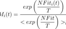
Sigma scaling preserves the differences between masses at more or less than a constant value over computa-tional process of the algorithm, but, there should be some changes in differences between masses in differ-ent times in a run. At the beginning of the algorithm, we want to have agents with low standard deviation in their masses, and later we want to have masses with more standard deviation. We can use the Boltzmann function to achieve this goal. This method is similar to the simulated annealing and uses the temperature parameter [30] . At the beginning of the algorithm, the temperature is high and is gradually reduced. A typical implementation of this method uses in the following equation.
Mi(t) =
exp
N F it
i(t)
T
< exp
N F it
T
>t
(13)
WhereMi(t) is the mass of agentiat timet,<>t
denotes the average over the all agents in timetand
T denotes the temperature which is a decreasing func-tion of time.T can be defined as a linear or exponen-tial function [30] . According to [31] we defineT as following:
T = 0.2
ln(t) (14)
Boltzmann function simulates the process of slow cooling of molten metal to reach the optimal value, which is the minimum, in a minimization problem. The cooling phenomenon is simulated by monitoring a temperature like the parameter introduced in Boltz-mann probability distribution. This method suggests that a system at a higher temperature visits more of the phase space, whereas at a lower temperature the probability of visiting points less favorable than the global minimum is lower. Furthermore, as described in [27] , Boltzmann function is translation invariant, and although this method is not scale invariant, any change in the scale can be offset by multiplying the temperature parameter by the scaling constant. Thus,
by controlling and monitoring the temperature T and assuming that the search process follows Boltzmann probability distribution, the convergence of the algo-rithm and exploration and exploitation abilities of the algorithm are controlled [32].
These new functions for mass calculation are exam-ined and compared with the original mass calculation function in the next section.
4
Experimental Results
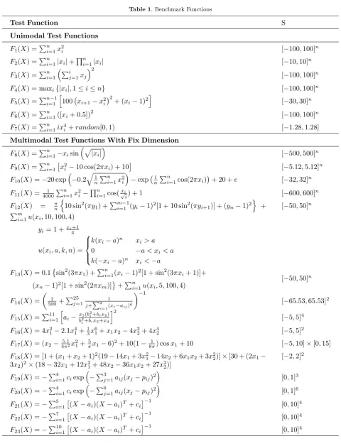
To evaluate the performance of our approaches and compare the results with other similar algorithms, we examined it on two sets of standard benchmark functions. The first set contains 23 test functions which are divided into two groups: unimodal (F1−F7) and
multimodal functions (F8−F23) and are shown in
Table 1. In this table,ndenotes the dimension of the function andS⊆Rn is the search space. Complete
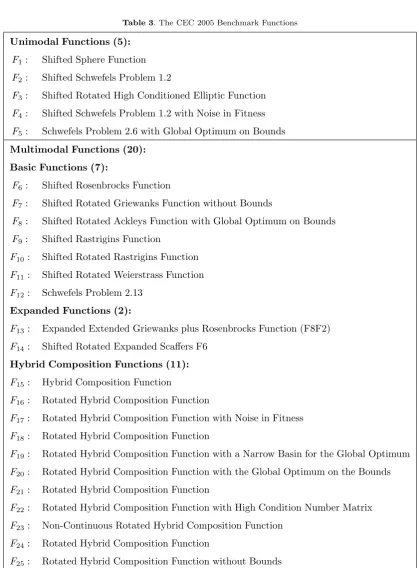
descriptions of these functions can be found in [19] and [20]. The second set includes 25 standard test functions of CEC 2005 which are divided into three categories: unimodal (F1−F5), basic multimodal (F6−F14),
and hybrid composition multimodal functions (F15− F25). These functions are summarized in Table tbl3.
Additional details about these functions can be found in [33] , [34] .
In unimodal functions, the rate of convergence is more important than the final result of the optimiza-tion, because there are some methods designed to op-timize unimodal functions. But, multimodal functions have many local optima. Thus, optimizing these func-tions is too difficult. In this kind of funcfunc-tions, the final result is more important, because it shows the ability of algorithm in escaping from local optima. More de-scription about these kinds of functions can be found in [19] and [22].
4.1 Experimental Results on the Standard Benchmark Functions
The performances of approaches which are introduced in this paper for mass calculation with Sigma Scal-ing (SSGSA) and Boltzmann selection (BSGSA) are compared with some popular optimization algorithms such as Real Genetic Algorithm (RGA) [35] , Particle Swarm Optimization algorithm (PSO) [36] , Gravita-tional Particle Swarm algorithm (GPS) [37] and stan-dard GSA. In all cases, the number of agents,i.e.the population size is set to 50 (N = 50), the maximum number of iteration is 1000 for all functions except for multimodal low dimensional functions (F7−F10)
which is 500 and the dimensions for functionsF1−F13
Table 1. Benchmark Functions
Test Function S
Unimodal Test Functions
F1(X) =P
n i=1x
2
i [−100,100]n
F2(X) =P
n
i=1|xi|+Q n
i=1|xi| [−10,10]n
F3(X) =P
n i=1
Pi
j=1xj
2
[−100,100]n
F4(X) = maxi{|xi|,1≤i≤n} [−100,100]n
F5(X) =Pni=1−1 h
100 xi+1−x2i
2
+ (xi−1)2
i
[−30,30]n
F6(X) =P
n
i=1([xi+ 0.5])
2
[−100,100]n
F7(X) =P
n i=1ix
4
i +random[0,1) [−1.28,1.28]
Multimodal Test Functions With Fix Dimension
F8(X) =P
n
i=1−xisin
p
|xi|
[−500,500]n
F9(X) =Pni=1x2i −10 cos(2πxi) + 10 [−5.12,5.12]n
F10(X) =−20 exp
−0.2
q 1
n
Pn i=1x
2
i
−exp 1nPn
i=1cos(2πxi)
+ 20 +e [−32,32]n
F11(X) =40001 P
n i=1x
2
i −
Qn
i=1cos(
xi √
i) + 1 [−600,600]
n
F12(X) = πn n
10 sin2(πy1) +P
m−1
i=1 (yi−1)2[1 + 10 sin2(πyi+1)] + (yn−1)2
o
+
Pm
i=1u(xi,10,100,4)
[−50,50]n
yi= 1 + xi4+1
u(xi, a, k, n) =
k(xi−a)n xi > a
0 −a < xi< a
k(−xi−a)n xi <−a
F13(X) = 0.1sin2(3πx1) +Pni=1(xi−1)2[1 + sin2(3πxi+ 1)]+
(xn−1)2[1 + sin2(2πxm)] +Pni=1u(xi,5,100,4)
[−50,50]n
F14(X) = 1 500+ P25 j=1 1
j+P2
i=1(xi−aij) 6
−1
[−65.53,65.53]2
F15(X) =P11i=1 h
ai−x1(b
2
i+bix2)
b2
i+bix3+x4
i2
[−5,5]4 F16(X) = 4x21−2.1x41+13x
6
1+x1x2−4x22+ 4x42 [−5,5]2
F17(X) = (x2−45π.12x 2
1+5πx1−6)
2+ 10(1− 1
8π) cosx1+ 10 [−5,10]×[0,15]
F18(X) = [1 + (x1+x2+ 1)2(19−14x1+ 3x12−14x2+ 6x1x2+ 3x22)]×[30 + (2x1−
3x2)2×(18−32x1+ 12x12+ 48x2−36x1x2+ 27x22)]
[−2,2]2
F19(X) =− P4
i=1ciexp
−P3j=1aij(xj−pij)2
[0,1]3 F20(X) =−
P4
i=1ciexp
−P6j=1aij(xj−pij)2
[0,1]6 F21(X) =−
P5
i=1
(X−ai)(X−ai)T+ci
−1
[0,10]4 F22(X) =−
P7
i=1
(X−ai)(X−ai)T+ci
−1
[0,10]4 F23(X) =−
P10
i=1
(X−ai)(X−ai)T+ci
−1
0 100 200 300 400 500 600 700 800 900 1000 Iteration
-4000 -3800 -3600 -3400 -3200 -3000 -2800 -2600 -2400
Best-so-far
F8
BSGSA SSGSA GSA
Figure 2. Comparison of the Performances of GSA, SSGSA and BSGSA for Minimization ofF8 withn= 30.
In RGA, the probability of crossover is set to 0.3 (Pc= 0.3) and the probability of mutation is set to 0.1
(Pm= 0.1). In this algorithm, roulette wheel selection
is used. In PSO, the two positive constantc1andc2
are set to 2 and inertia factorωis decreased linearly from 0.9 to 0.2. The parameters in GPS are set as [37]. In GSA, SSGSA, and BSGSA,αis set to 20 andG0
is set to 100 andK0is equal to the total number of
agents (N) and is decreased linearly to 1.
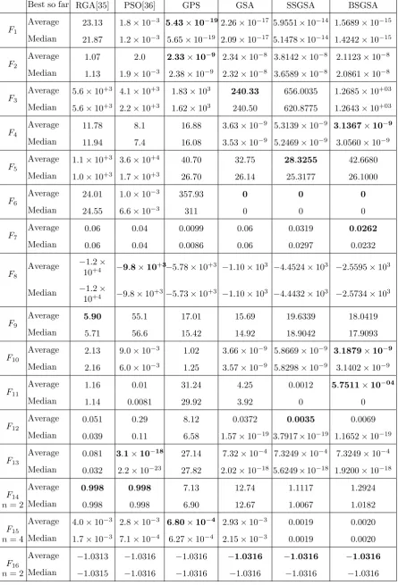
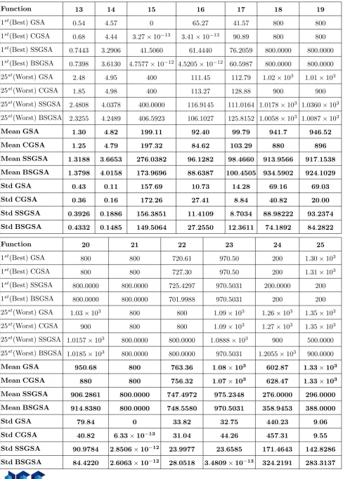
The average and the median of the best solutions on 30 independent runs are computed and reported in Table 2. In this table, the best results are boldfaced. As Table 2 shows, GSA, SSGSA and BSGSA provide better answers for all these standard benchmark func-tions than that of other heuristic algorithms except
F1, F2, F9 andF13−F15. For F1, F2 andF15, GPS
achieves the best results. ForF13andF14, PSO has
the best performance while onF9, the RGA algorithm
performs better. The performances of GSA, SSGSA, and BSGSA are the same forF6, F16−F20, F22and F23whereas for functionsF4, F7, F11andF21, the
per-formance of BSGSA is better. The good perper-formance of SSGSA can be seen in solvingF5andF12.
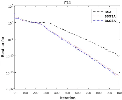
Figures 2 and 3 illustrate the comparison of perfor-mance of GSA, SSGSA, and BSGSA for functionsF8
andF11. These are multimodal functions with many
local optima and they are useful to evaluate the abil-ity of search algorithm in escaping from poor local optima. As these figures illustrate, at the beginning of the GSA, there are major difference between the masses, as mentioned in the previous section. So, the exploration power of the algorithm is low and GSA gets trapped in the local optima. But, in the proposed methods, scaling functions used to control the explo-ration and exploitation abilities of the algorithm. At the beginning of the algorithm, scaling functions in-crease the exploration power of the algorithm. This
0 100 200 300 400 500 600 700 800 900 1000 Iteration
10-20 10-15 10-10 10-5 100 105
Best-so-far
F11
GSA SSGSA BSGSA
Figure 3. Comparison of the Performances of GSA, SSGSA and BSGSA for Minimization ofF11 withn= 30.
feature prevents the algorithm from getting trapped in local optima and helps it to explore the search space. On the other hand, towards the end of the algorithm, using the scaling functions tends to decrease the ex-ploration ability of the algorithm and increase the exploitation power of the algorithm and helps to con-verge to a better solution and search the feasible area around it. As a result, SSGSA, and BSGSA, which use the scaling functions for their mass calculation to control their exploitation and exploration ability, can escape from local optima and provide better results than GSA.
4.2 Experimental Results on the CEC 2005
The performances of the proposed algorithms are also tested on the standard benchmark functions of CEC 2005 which are summarized in Table 3 and are compared with standard GSA and Clustered GSA (CGSA). The parameters of CGSA are set as described
in [25].
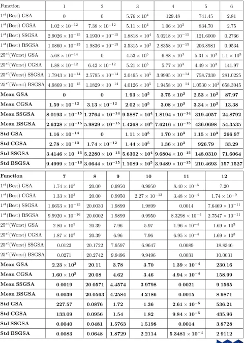
Table 4 contains the resulting error values of these algorithms on these standard test functions after 1e+5 fitness evaluations (FEs) with dimension 10 (n=10). The best (1st), the worst (25th), mean and the
stan-dard deviation of the error values on 25 independent runs are computed and shown in this table. The re-sults of GSA and CGSA are taken from [25].
In this reference, the error values of CGSA on these test functions are computed and reported after 92160 fitness evaluations. In Table 4, the mean and standard deviation of the error values after 92160 FEs for CGSA and 1e+5 FEs for other algorithms are boldfaced.
Table 2. The Results of Benchmark Functions of Table 1.
Best so far RGA[35] PSO[36] GPS GSA SSGSA BSGSA
F1
Average 23.13 1.8×10⁻³ 5.43×10−192.26×10⁻¹⁷ 5.9551×10⁻¹⁴ 1.5689×10⁻¹⁵
Median 21.87 1.2×10⁻³ 5.65×10⁻¹⁹ 2.09×10⁻¹⁷ 5.1478×10⁻¹⁴ 1.4242×10⁻¹⁵
F2
Average 1.07 2.0 2.33×10⁻⁹ 2.34×10⁻⁸ 3.8142×10⁻⁸ 2.1123×10⁻⁸
Median 1.13 1.9×10⁻³ 2.38×10⁻⁹ 2.32×10⁻⁸ 3.6589×10⁻⁸ 2.0861×10⁻⁸
F3
Average 5.6×10+3 4.1×10+3 1.83×10³ 240.33 656.0035 1.2685×10+03
Median 5.6×10+3 2.2×10+3 1.62×10³ 240.50 620.8775 1.2643×10+03
F4
Average 11.78 8.1 16.88 3.63×10⁻⁹ 5.3139×10⁻⁹ 3.1367×10⁻⁹
Median 11.94 7.4 16.08 3.53×10⁻⁹ 5.2469×10⁻⁹ 3.0560×10⁻⁹
F5
Average 1.1×10+3 3.6×10+4 40.70 32.75 28.3255 42.6680
Median 1.0×10+3 1.7×10+3 26.70 26.14 25.3177 26.1000
F6
Average 24.01 1.0×10⁻³ 357.93 0 0 0
Median 24.55 6.6×10⁻³ 311 0 0 0
F7
Average 0.06 0.04 0.0099 0.06 0.0319 0.0262
Median 0.06 0.04 0.0086 0.06 0.0297 0.0232
F8
Average −1.2×
10+4 −9.8×10
+3−5.78×10+3 −1.10×10³ −4.4524×10³ −2.5595×10³
Median −1.2×
10+4 −9.8×10+3−5.73×10+3 −1.10×10³ −4.4432×10³ −2.5734×10³
F9
Average 5.90 55.1 17.01 15.69 19.6339 18.0419
Median 5.71 56.6 15.42 14.92 18.9042 17.9093
F10
Average 2.13 9.0×10⁻³ 1.02 3.66×10⁻⁹ 5.8669×10⁻⁹ 3.1879×10⁻⁹
Median 2.16 6.0×10⁻³ 1.25 3.57×10⁻⁹ 5.8298×10⁻⁹ 3.1402×10⁻⁹
F11
Average 1.16 0.01 31.24 4.25 0.0012 5.7511×10−04
Median 1.14 0.0081 29.92 3.92 0 0
F12
Average 0.051 0.29 8.12 0.0372 0.0035 0.0069
Median 0.039 0.11 6.58 1.57×10⁻¹⁹ 3.7917×10⁻¹⁹ 1.1652×10⁻¹⁹
F13
Average 0.081 3.1×10⁻¹⁸ 27.14 7.32×10⁻⁴ 7.3249×10⁻⁴ 7.3249×10⁻⁴
Median 0.032 2.2×10⁻²³ 27.82 2.02×10⁻¹⁸ 5.6249×10⁻¹⁸ 1.9200×10⁻¹⁸
F14
Average 0.998 0.998 7.13 12.74 1.1117 1.2924
n= 2 Median 0.998 0.998 6.90 12.67 1.0067 1.0182
F15
Average 4.0×10⁻³ 2.8×10⁻³ 6.80×10⁻⁴ 2.93×10⁻³ 0.0019 0.0020
n= 4 Median 1.7×10⁻³ 7.1×10⁻⁴ 6.27×10⁻⁴ 2.15×10⁻³ 0.0019 0.0020
F16
Average −1.0313 −1.0316 −1.0316 −1.0316 −1.0316 −1.0316
Table 2 Continued. The Results of Benchmark Functions of Table 1.
Best so far RGA[35] PSO[36] GPS GSA SSGSA BSGSA
F17
Average 0.3996 0.3979 0.3979 0.3979 0.3979 0.3979
n= 2 Median 0.3980 0.3979 0.3979 0.3979 0.3979 0.3979
F18
Average 5.70 3.00 3.00 3.00 3.0000 3.0000
n= 2 Median 3.0 3.00 3.00 3.00 3.0000 3.0000
F19
Average −3.8627 −3.8628 −3.8628 −3.8628 −3.8628 −3.8628
n= 3 Median −3.8628 −3.8628 −3.8628 −3.8628 −3.8628 −3.8628
F20
Average −3.3099 −3.2369 −3.2621 −3.3220 −3.3220 −3.3220
n= 6 Median −3.3217 −3.2031 −3.2625 −3.3220 −3.3220 −3.3220
F21
Average −5.6605 −6.6290 −6.8232 −5.9200 −7.0412 −7.0584
n= 4 Median −2.6824 −5.1008 −10.1532 −2.6829 −10.1532 −10.1532
F22
Average −7.3421 −9.1118 −9.3842 −10.403 −10.4029 −10.1479
n= 4 Median −10.3932 −10.402 −10.4029 −10.403 −10.4029 −10.4029
F23
Average −6.2541 −9.7634 −10.0575 −10.5364 −10.5364 −10.5364
n= 4 Median −4.5054 −10.536 −10.5364 −10.5364 −10.5364 −10.5364
0 200 400 600 800 1000 1200 1400 1600 1800 2000
Iteration 10-15
10-10 10-5 100 105
Best-so-far
F7
GSA SSGSA BSGSA
Figure 4. Comparison of the Performances of GSA, SSGSA and BSGSA for Minimization ofF7 withn= 10.
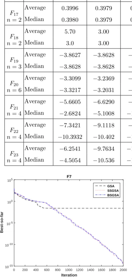
show for unimodal functions, the proposed algorithms have a good performance for functions F3, F4 and F5. However, these algorithms could not achieve
op-timal solutions forF1andF2which GSA could find
the exact answer for these functions. For basic mul-timodal functions, SSGSA and BSGSA have better performance than GSA and CSGSA for F7, F8, F12
andF14. Finally, for hybrid composition multimodal
functions, the proposed algorithms performed well for
F15, F17, F19, F21, F22, F23, F24 and F25. The CGSA
has a better performance forF16, F18andF20and the
0 200 400 600 800 1000 1200 1400 1600 1800 2000
Iteration 10-15
10-10 10-5 100 105
Best-so-far
F11
GSA SSGSA BSGSA
Figure 5. Comparison of the Performances of GSA, SSGSA and BSGSA for Minimization ofF11 withn= 10.
results of SSGSA and BSGSA are close to the CGSA results. Also, Figures 4 and 5 illustrate the compari-son of performance of GSA, SSGSA, and BSGSA for functionsF7andF11which are multimodal functions
Table 3. The CEC 2005 Benchmark Functions
Unimodal Functions (5):
F1: Shifted Sphere Function F2: Shifted Schwefels Problem 1.2
F3: Shifted Rotated High Conditioned Elliptic Function F4: Shifted Schwefels Problem 1.2 with Noise in Fitness F5: Schwefels Problem 2.6 with Global Optimum on Bounds
Multimodal Functions (20):
Basic Functions (7):
F6: Shifted Rosenbrocks Function
F7: Shifted Rotated Griewanks Function without Bounds
F8: Shifted Rotated Ackleys Function with Global Optimum on Bounds F9: Shifted Rastrigins Function
F10: Shifted Rotated Rastrigins Function F11: Shifted Rotated Weierstrass Function F12: Schwefels Problem 2.13
Expanded Functions (2):
F13: Expanded Extended Griewanks plus Rosenbrocks Function (F8F2) F14: Shifted Rotated Expanded Scaffers F6
Hybrid Composition Functions (11):
F15: Hybrid Composition Function
F16: Rotated Hybrid Composition Function
F17: Rotated Hybrid Composition Function with Noise in Fitness F18: Rotated Hybrid Composition Function
F19: Rotated Hybrid Composition Function with a Narrow Basin for the Global Optimum F20: Rotated Hybrid Composition Function with the Global Optimum on the Bounds F21: Rotated Hybrid Composition Function
F22: Rotated Hybrid Composition Function with High Condition Number Matrix F23: Non-Continuous Rotated Hybrid Composition Function
F24: Rotated Hybrid Composition Function
Table 4. Minimization Results on Tests Functions After 92160 FEs for CGSA and 1e+5 FEs for Other Algorithms
Function 1 2 3 4 5 6
1st(Best) GSA
0 0 5.76×10⁴ 129.48 741.45 2.81
1st(Best) CGSA
1.02×10⁻¹² 7.38×10⁻¹² 5.11×10⁴ 1.06×10³ 834.70 2.75
1st(Best) SSGSA
2.9026×10⁻¹⁵ 3.1930×10⁻¹⁵ 1.8818×10⁴ 5.0218×10⁻¹⁵ 121.6000 0.2766
1st(Best) BSGSA 1.0860×10⁻¹⁵ 1.9836×10⁻¹⁵ 3.5315×10³ 2.8358×10⁻¹⁵ 206.8981 0.9534
25st(Worst) GSA 5.68×10⁻¹⁴ 0 4.53×10⁵ 6.88×10³ 5.31×10³ 1.1×10³
25st(Worst) CGSA
1.88×10⁻¹² 6.42×10⁻¹² 5.21×10⁵ 5.77×10³ 4.49×10³ 141.97 25st(Worst) SSGSA 1
.7943×10−14 2.5795×10⁻¹⁴ 2.0495×10⁵ 3.9995×10⁻¹⁴ 758.7330 281.0225 25st(Worst) BSGSA 4
.9869×10−15 1.1829×10⁻¹⁴ 4.0126×10⁵ 1.9458×10⁻¹⁴ 1.0530×10³ 658.3045
Mean GSA 0 0 1.93×10⁵ 3.75×10³ 2.53×10³ 87.97
Mean CGSA 1.59×10⁻¹² 3.13×10⁻¹² 2.02×10⁵ 3.08×10³ 3.34×10³ 13.38
Mean SSGSA 8.0193×10⁻¹⁵ 1.2764×10⁻¹⁴ 9.5887×10⁴ 1.8194×10⁻¹⁴ 319.4057 24.8792
Mean BSGSA 2.6328×10⁻¹⁵ 5.9829×10⁻¹⁵ 1.4268×10⁵ 7.6216×10⁻¹⁵ 436.0698 54.3535
Std GSA 1.16×10⁻¹⁴ 0 1.11×10⁵ 1.70×10³ 1.15×10³ 266.97
Std CGSA 2.78×10⁻¹³ 1.74×10⁻¹² 1.44×10⁵ 1.36×10³ 926.79 33.29
Std SSGSA 3.4146×10⁻¹⁵ 5.2280×10⁻¹⁵ 5.6302×10⁴ 9.6804×10⁻¹⁵ 148.0310 71.6064
Std BSGSA 9.4999×10⁻¹⁶ 3.0644×10⁻¹⁵ 1.1089×10⁵ 3.9489×10⁻¹⁵ 210.4693 157.1527
Function 7 8 9 10 11 12
1st(Best) GSA 1.74×10³ 20.00 0.9950 0.9950 8.40×10⁻⁵ 7.20
1st(Best) CGSA 1.33×10³ 20.00 0.9950 2.27×10⁻¹³ 3.48×10⁻⁴ 1.74×10⁻⁹
1st(Best) SSGSA
1.6653×10⁻¹⁵ 20.0030 1.9899 1.9899 0.0014 7.6469×10⁻¹¹ 1st(Best) BSGSA
9.9920×10⁻¹⁶ 20.0002 1.9899 0.9950 8.3298×10⁻⁴ 2.7547×10⁻¹¹ 25st(Worst) GSA
2.80×10³ 20.39 7.96 5.97 1.96×10⁻⁴ 1.69×10³
25st(Worst) CGSA
1.87×10³ 20.39 6.96 7.96 6.95×10⁻⁴ 1.69×10³
25st(Worst) SSGSA
0.0123 20.1722 7.9597 6.9647 0.0089 18.8346 25st(Worst) BSGSA 0.0271 20.2742 9.9496 9.9496 0.0031 10.0031
Mean GSA 2.23×10³ 20.11 3.78 3.70 1.39×10⁻⁴ 230.16
Mean CGSA 1.60×10³ 20.08 4.62 3.46 4.94×10⁻⁴ 158.99
Mean SSGSA 0.0019 20.0571 4.4574 3.9798 0.0021 9.1565
Mean BSGSA 0.0039 20.0563 4.2584 4.2186 0.0015 8.9871
Std GSA 227.57 0.0876 1.72 1.36 2.61×10⁻⁵ 536.21
Std CGSA 133.09 0.0956 1.54 1.82 9.84×10⁻⁵ 435.96
Std SSGSA 0.0040 0.0481 1.5763 1.5198 0.0014 3.8728
Table 4 Continued. Minimization Results on Tests Functions After 92160 FEs for CGSA and 1e+5 FEs for Other Algorithms
Function 13 14 15 16 17 18 19
1st(Best) GSA
0.54 4.57 0 65.27 41.57 800 800
1st(Best) CGSA
0.68 4.44 3.27×10⁻¹³ 3.41×10⁻¹³ 90.89 800 800
1st(Best) SSGSA
0.7443 3.2906 41.5060 61.4440 76.2059 800.0000 800.0000 1st(Best) BSGSA 0.7398 3.6130 4.7577×10⁻¹² 4.5205×10⁻¹² 60.5987 800.0000 800.0000
25st(Worst) GSA 2.48 4.95 400 111.45 112.79 1.02×10³ 1.01×10³
25st(Worst) CGSA
1.85 4.98 400 113.27 128.88 900 900
25st(Worst) SSGSA
2.4808 4.0378 400.0000 116.9145 111.0164 1.0178×10³ 1.0360×10³ 25st(Worst) BSGSA
2.3255 4.2489 406.5923 106.1027 125.8152 1.0058×10³ 1.0087×10³
Mean GSA 1.30 4.82 199.11 92.40 99.79 941.7 946.52
Mean CGSA 1.25 4.79 197.32 84.62 103.29 880 896
Mean SSGSA 1.3188 3.6653 276.0382 96.1282 98.4660 913.9566 917.1538
Mean BSGSA 1.3798 4.0158 173.9696 88.6387 100.4505 934.5902 924.1029
Std GSA 0.43 0.11 157.69 10.73 14.28 69.16 69.03
Std CGSA 0.36 0.16 172.26 27.41 8.84 40.82 20.00
Std SSGSA 0.3926 0.1886 156.3851 11.4109 8.7034 88.98222 93.2374
Std BSGSA 0.4332 0.1485 149.5064 27.2550 12.3611 74.1892 84.2822
Function 20 21 22 23 24 25
1st(Best) GSA 800 800 720.61 970.50 200 1.30×10³
1st(Best) CGSA 800 800 727.30 970.50 200 1.31×10³
1st(Best) SSGSA
800.0000 800.0000 725.4297 970.5031 200.0000 200 1st(Best) BSGSA
800.0000 800.0000 701.9988 970.5031 200 200
25st(Worst) GSA
1.03×10³ 800 800 1.09×10³ 1.26×10³ 1.35×10³
25st(Worst) CGSA
900 800 800 1.09×10³ 1.27×10³ 1.35×10³
25st(Worst) SSGSA 1
.0157×103 800.0000 800.0000 1.0888×10³ 900 500.0000
25st(Worst) BSGSA 1.0185×10³ 800.0000 800.0000 970.5031 1.2055×10³ 900.0000
Mean GSA 950.68 800 763.36 1.08×10³ 602.87 1.33×10³
Mean CGSA 880 800 756.32 1.07×10³ 628.47 1.33×10³
Mean SSGSA 906.2861 800.0000 747.4972 975.2348 276.0000 296.0000
Mean BSGSA 914.8380 800.0000 748.5580 970.5031 358.9453 388.0000
Std GSA 79.84 0 33.82 32.75 440.23 9.06
Std CGSA 40.82 6.33×10⁻¹³ 31.04 44.26 457.31 9.55
Std SSGSA 90.9784 2.8506×10⁻¹² 23.9977 23.6585 171.4643 142.8286
5
Conclusion
In this paper, scaling functions, i.e. Sigma scaling and Boltzmann selection functions are used for mass calculation in the computational process of GSA to balance the exploitation and exploration power of the algorithm and improve the performance of the algo-rithm. The proposed functions are evaluated on two sets of standard test functions including unimodal functions and multimodal functions and the results are compared with the standard GSA, genetic algorithm, particle swarm optimization, gravitational particle swarm optimization algorithm, and clustered-GSA. The experimental results show that the proposed func-tions despite the simplicity of their implementation compared to other methods, are a remarkable way to improve the results. In future, these methods can be used to solve some different optimization problems.
References
[1] F Musharavati and AMS Hamouda. Simulated annealing with auxiliary knowledge for process planning optimization in reconfigurable manufac-turing. Robotics and Computer-Integrated Manu-facturing, 28(2):113–131, 2012.
[2] Qingbao Zhu, Jun Hu, and Larry Henschen. A new moving target interception algorithm for mobile robots based on sub-goal forecasting and an improved scout ant algorithm. Applied Soft Computing, 13(1):539–549, 2013.
[3] Konstantinos Ioannidis, G Ch Sirakoulis, and Ioannis Andreadis. Cellular ants: A method to create collision free trajectories for a cooperative robot team. Robotics and Autonomous Systems, 59(2):113–127, 2011.
[4] Hongwei Ding, Ly`es Benyoucef, and Xiaolan Xie. A simulation-based multi-objective genetic algo-rithm approach for networked enterprises opti-mization. Engineering Applications of Artificial Intelligence, 19(6):609–623, 2006.
[5] U G¨uven¸c, Y S¨onmez, S Duman, and N Y¨or¨ukeren. Combined economic and emission dispatch solu-tion using gravitasolu-tional search algorithm. Scien-tia Iranica, 19(6):1754–1762, 2012.
[6] Pei-Chann Chang, Jyun-Jie Lin, and Chen-Hao Liu. An attribute weight assignment and par-ticle swarm optimization algorithm for medical database classifications. Computer methods and programs in biomedicine, 107(3):382–392, 2012. [7] Barnali Sahu and Debahuti Mishra. A novel
feature selection algorithm using particle swarm optimization for cancer microarray data.Procedia Engineering, 38:27–31, 2012.
[8] Debahuti Mishra. Discovery of overlapping pat-tern biclusters from gene expression data using
hash based pso. Procedia Technology, 4:390–394, 2012.
[9] Daniela Di Serafino, Susana Gomez, Leopoldo Milano, Filippo Riccio, and Gerardo Toraldo. A genetic algorithm for a global optimization problem arising in the detection of gravitational waves. Journal of Global Optimization, 48(1): 41–55, 2010.
[10] Hee-Su Kim and Sung-Bae Cho. Application of interactive genetic algorithm to fashion design. Engineering applications of artificial intelligence, 13(6):635–644, 2000.
[11] XiaoHong Han and XiaoMing Chang. Chaotic secure communication based on a gravitational search algorithm filter. Engineering Applications of Artificial Intelligence, 25(4):766–774, 2012. [12] Esmat Rashedi, Hossien Nezamabadi-Pour, and
Saeid Saryazdi. Filter modeling using gravita-tional search algorithm.Engineering Applications of Artificial Intelligence, 24(1):117–122, 2011. [13] Chengtao Guo, Jiang Zhibin, Huai Zhang, and
Na Li. Decomposition-based classified ant colony optimization algorithm for scheduling semicon-ductor wafer fabrication system. Computers & Industrial Engineering, 62(1):141–151, 2012. [14] Soumitra Mondal, Aniruddha Bhattacharya, and
Sunita Halder nee Dey. Multi-objective economic emission load dispatch solution using gravita-tional search algorithm and considering wind power penetration. International Journal of Elec-trical Power & Energy Systems, 44(1):282–292, 2013.
[15] Di Hu, Ali Sarosh, and Yun-Feng Dong. An im-proved particle swarm optimizer for parametric optimization of flexible satellite controller. Ap-plied Mathematics and Computation, 217(21): 8512–8521, 2011.
[16] T Ganesan, I Elamvazuthi, Ku Zilati Ku Shaari, and P Vasant. Swarm intelligence and gravita-tional search algorithm for multi-objective opti-mization of synthesis gas production. Applied Energy, 103:368–374, 2013.
[17] Vijay Kumar, Jitender Kumar Chhabra, and Di-nesh Kumar. Automatic cluster evolution using gravitational search algorithm and its application on image segmentation.Engineering Applications of Artificial Intelligence, 29:93–103, 2014. [18] Weiguo Zhao. Adaptive image enhancement
based on gravitational search algorithm.Procedia Engineering, 15:3288–3292, 2011.
[19] Esmat Rashedi, Hossein Nezamabadi-Pour, and Saeid Saryazdi. Gsa: a gravitational search algo-rithm. Information sciences, 179(13):2232–2248, 2009.
algorithm. Natural Computing, 9(3):727–745, 2010.
[21] Mohadeseh Soleimanpour Moghadam, Hossein Nezamabadi-Pour, and Malihe M Farsangi. A quantum behaved gravitational search algorithm. 2012.
[22] Mohammad Doraghinejad and Hossein Nezamabadi-pour. Black hole: A new operator for gravitational search algorithm. International Journal of Computational Intelligence Systems, 7 (5):809–826, 2014.
[23] S Sarafrazi, H Nezamabadi-Pour, and S Saryazdi. Disruption: a new operator in gravitational search algorithm. Scientia Iranica, 18(3):539–548, 2011. [24] FS Saeidi-Khabisi and Esmat Rashedi. Fuzzy gravitational search algorithm. Proceedings 2nd international econference on computer and knowl-edge engineering, pages 156–160, 2012.
[25] Masumeh Shams, Esmat Rashedi, and Ahmad Hakimi. Clustered-gravitational search algorithm and its application in parameter optimization of a low noise amplifier. Applied Mathematics and Computation, 258:436–453, 2015.
[26] Norlina Mohd Sabri, Mazidah Puteh, and Mo-hamad Rusop Mahmood. A review of gravita-tional search algorithm. Int. J. Advance. Soft Comput. Appl, 5(3):1–39, 2013.
[27] Lance D Chambers.Practical handbook of genetic algorithms: complex coding systems, volume 3. CRC press, 1998.
[28] David E Golberg. Genetic algorithms in search, optimization, and machine learning. Addion wes-ley, 1989:102, 1989.
[29] Zbigniew Michalewicz. Gas: What are they? In Genetic algorithms+ data structures= evolution
programs, pages 13–30. Springer, 1994.
[30] Melanie Mitchell. An introduction to genetic algorithms (complex adaptive systems). 1998. [31] Dimitris Bertsimas, John Tsitsiklis, et al.
Simu-lated annealing. Statistical science, 8(1):10–15, 1993.
[32] Singiresu S Rao and SS Rao. Engineering op-timization: theory and practice. John Wiley & Sons, 2009.
[33] Jane-Jing Liang, Ponnuthurai Nagaratnam Sug-anthan, and Kalyanmoy Deb. Novel composition test functions for numerical global optimization. In Proceedings 2005 IEEE Swarm Intelligence Symposium, 2005. SIS 2005., pages 68–75. IEEE, 2005.
[34] Ponnuthurai N Suganthan, Nikolaus Hansen, Jing J Liang, Kalyanmoy Deb, YP Chen, Anne Auger, and S Tiwari. Problem definitions and evaluation criteria for the cec 2005 special ses-sion on real-parameter optimization. Technical Report, Nanyang Technological University,
Singa-pore, May 2005 AND KanGAL Report 2005005, IIT Kanpur, India, 2005.
[35] Randy L Haupt and Sue Ellen Haupt. Practical genetic algorithms. John Wiley & Sons, 2004. [36] James Kennedy. Particle swarm optimization. In
Encyclopedia of machine learning, pages 760–766. Springer, 2011.
[37] Hsing-Chih Tsai, Yaw-Yauan Tyan, Yun-Wu Wu, and Yong-Huang Lin. Gravitational particle swarm. Applied Mathematics and Computation, 219(17):9106–9117, 2013.
Sepehr Ebrahimi Moodreceived his Bach-elor’s degree in Computer Science from Shahid Beheshti University Tehran, Iran in 2012 and his master’s degree in Computer Science from Sharif University of Technology, Iran in 2014. Now he is a PhD student in Computer Sci-ence at Shahid Bahonar University of Ker-man, Iran. His main interests are artificial in-telligence, theory of computation, and image processing.
Esmat Rashedireceived her B.Sc. degree in Electrical Engineering, and her M.Sc. and Ph.D. degree in Communication engineering from Shahid Bahonar University of Kerman, Iran, in 2004, 2007, and 2013, respectively. Now she is an assistant Professor at Gradu-ate University of Advanced Technology. Her research interests include heuristic optimiza-tion algorithms, soft computing, evoluoptimiza-tionary computaoptimiza-tion, image processing, and pattern recognition.
Mohammad Masoud Javidireceived his
![Figure 1. The General Principle of GSA [19].](https://thumb-us.123doks.com/thumbv2/123dok_us/40038.2004510/3.595.326.521.75.390/figure-the-general-principle-of-gsa.webp)