Mathematical Model for Bi-objective Maximal Hub Covering Problem with Periodic Variations of Parameters

Please cite this article as: Y. Khosravian, A. Shahandeh, G. Moslehi, Mathematical Model for Bi-objective Maximal Hub Covering Problem with Periodic Variations of Parameters, International Journal of Engineering (IJE), IJE TRANSACTIONS A: Basics Vol. 32, No. 7, (July 2019) 964-975

International Journal of Engineering

Mathematical Model for Bi-objective Maximal Hub Covering Problem with Periodic

Variations of Parameters

Y. Khosravian Ghadikolaei*, A. Shahandeh Nookabadi, G. Moslehi

Department of Industrial and Systems Engineering, Isfahan University of Technology, Isfahan, Iran

P A P E R I N F O

Paper history: Received 04 March 2019

Received in revised form 30 April 2019 Accepted 03 May 2019

Keywords:

Maximal Hub Covering Dynamic Hub Location Multi-period Hub Location ε-constraint Method Benders Decomposition

A B S T R A C T

T he problem of maximal hub covering as a challenging problem in operation research. Transportation programming seeks to find an optimal location of a set of hubs to reach maximum flow in a network. Since the main structure's parameters of the problem such as origin-destination flows, costs and travel time, change periodically in the real world applications, new issues arise in handling it. In this paper, to deal with the periodic variations of parameters, a bi-objective mathematical model is proposed for the single allocation multi-period maximal hub covering problem. T he ε-constraint approach has been applied to achieve non-dominated solutions. Given that the single-objective problem found in the ε-constraint method is computationally intractable. Benders decomposition algorithm by adding valid inequalities is developed to accelerate the solution process. Finally, the proposed method is carried out by CAB data set, and the results confirm the efficiency of it regarding optimality and running time.

doi: 10.5829/ije.2019.32.07a.09

1. INTRODUCTION1

In recent years, many shipping and telecommunication companies have tended to use hub networks for transferring flows between origins and destinations. Hub facilities are located in network nodes and provide services such as switching, sorting, and consolidation of flows. Using hubs can reduce network connections and thus reduce network construction costs . Also, with the use of special transport facilities between hubs, economic savings will be made in traveling costs. Hub location issues are commonly applied in air transport industries, postal delivery services, telecommunication services, container, and maritime transportation systems.

In general, the hub location problems (HLPs) can be divided into four categories, including p-hub median location problem, hub location problem with fixed costs, p-hub center problem and hub covering problems [1]. For the first time, Campbell [2] presented the

*Corresponding Aut hor Email: [email protected] (Y. Khosravian Ghadikolaei)

mathematical model of hub covering problem with single and multiple allocations. The difference between hub covering problems (HCPs) with other HLPs is the limitation of length or time or cost of the path of origin -destination (O/D) pairs. HCPs can be applied to the design of the distribution network of perishable goods and also the design of transportation networks with driving time limitation. HCPs are divided into two categories: Hub set-covering problem (HSCP) and Maximal-hub covering problem (MHCP). HSCP aims to determine the location of the hubs so that all O/D pairs are covered, and the total costs of establishing hubs are minimized. In MHCP, due to the limitations such as the number of fleets and available budgets, the goal is to maximize the amount of covered demand by locating a certain number of hubs.

Campbell [2] defined three types of coverage in HCPs. Each O/D pair (i,j) is covered by hubs k and l if:  The flow transmission cost (time or distance) from

origin i to destination j does not exceed a predetermined value.

hub l to destination j does not exceed a predetermined value.

 The flow transmission cost (time or distance) from origin i to hub k and from hub l to destination j does not exceed a predetermined value.

Karimi and Bashiri [3] presented models for HSCP and MHCP with type 2 coverage and provided two heuristic algorithms. Hwang and Lee [4] proposed a new mathematical formulation for the MHCP with fewer constraints and variables than the existing models. Also, they presented two heuristic algorithms to solve MHCP and confirmed them on the Civil Aeronautics Board (CAB) Dataset. The results showed that the algorithms are efficient regarding to solution quality and solving time. Jabalameli et al. [5] proposed two mathematical formulas for MHCP with a single allocation and developed a simulated annealing algorithm to solve it. Ebrahimi-zade et al. [6] presented a non-linear multi-objective model for MHCP by considering uncertainty. The model was provided for single and multiple allocation types and it was also linearized. Since there is the possibility of interruptions in each O/D path in the real world, maximizing the reliability in the weakest network path were also considered along with the common goal of maximizing the amount of covered flow. Also, the modified non-dominated sorting genetic algorithm II (NSGAII) was used to solve the problem. Pasandideh et al. [7] presented a bi-objective model for uncapacitated single allocation MHCP considering time-dependent reliabilities. They used the second type of coverage, and the objectives of the problem includ ing maximizing the flow and the reliability of the network. They transformed the proposed model to a single-objective model by goal attainment method. Because of the NP-hardness of the problem, the genetic algorithm was developed.

Bashiri and Rezanezhad [8] presented a multi-objective model for uncapacitated single allocation HSCP and used ε-constraint and NSGAII algorithms to solve the problem. The model aims to minimize the total investment and transportation costs, minimizes the maximum traveling time between pair of nodes, maximizes the total reliability of available paths and forces to allocate near nodes to more reliable hubs. Karimi, et al. [9] presented a mathematical formulation for capacitated single allocation HSCP in multi-modal network. They presented six valid inequalities to tight the linear programming lower bound and developed a heuristic based on the tabu search algorithm to solve the problem. Ebrahimi-zade, et al. [10] presented a bi-objective model for uncapacitated single allocation MHCP with uncertainty. They also used fuzzy multi-objective linear programming to solve the problem. The model aims to maximize flow and maximize reliability in the weakest path of the network. They assumed that the transportation time is a normal random variable.

Janković and Stanimirović [11] proposed a mathematical model for uncapacitated r-allocation MHCP. To solve the model, they used the general variable neighborhood search algorithm. Janković, et al. [12] presented different mathematical models for uncapacitated MHCP with single and multiple allocations. They used two different types of coverage (binary and partial) and general variable neighborhood search algorithm to solve the proposed models. Madani, et al. [13] presented a reliable bi-objective mathematical model for the single allocation MHCP. The objectives include maximizing the covered flow and minimizing congestion in the network. They used NSGAII algorithm to solve the proposed model and examin ed its effectiveness against multi-objective particle swarm optimization (MOPSO) and Epsilon constraint algorithms.

Several parameters influence the design of hub networks, such as O/D flows, hub capacity, the capacity of transportation facilities, costs, and traveling time. These parameters may change periodically in the future by some reasons such as seasonal variations, inflations and technology improvements. Regarding the periodic variations of parameters during the planning horizon, HLPs can be divided into static and multi-period (dynamic) issues. In static HLPs, it is assumed that the effective decision parameters are fixed and remain unchanged over the planning horizon . Therefore, the optimum locations of the hub facilities are fixed in the planned horizon. While in multi-period HLPs, it is assumed that the effective decision parameters change periodically and their values are constant in each period. In this situation, the planning horizon is divided into different periods, while the location of hub facilities can change in different periods. In this case, the obtained solution may not be optimal for each of the periods but it will be the best solution throughout the planning horizon, indeed.

Gelareh [14] thesis is one of the first studies in designing a multi-period hub network in public transport. He considered parameters such as demand, discount factor, the operational cost of the hubs, and the cost of opening and closing hubs are changed periodically. A few research has been conducted on multi-period hub location problems. In hub covering problems, only Ebrahimi-zade et al. [15] presented a mathematical formulation for multi-period hub set-covering problem, in which the coverage range is a decision variable. They considered parameters such as travel cost, opening and closing costs of hubs, hubs covering costs, and the income of closing hubs are changed periodically. Moreover, because of the NP-hardness of the proposed model, they developed a genetic algorithm to solve it.

which decision-making parameters will not change in the future, and mathematical models have been developed in a static environment. One of the primary reasons for this, is the high cost of constructing and launching hubs, which has made it impossible to make changes into the hub network. However, in some cases, the establishing cost of hubs is meager in comparison with the cost of routing flows (such as telecommunications networks) or the hub network service providers are not the infrastructure owner (such as airlines). So, in these contexts, the structure of the hub network can be changed over the planning horizon [16]. Also, even if changing the location of the hubs is impossible, we can adequately determine the flow path according to the periodic variations of the parameters.

In this study, to deal with the periodic variations of parameters, a mathematical formulation for the bi-objective multi-period maximal hub covering problem (BOMMHCP) is developed. Another contribution in the model is the simultaneous consideration of the goals of maximizing the covered demand of all O/D Pairs and minimizing the cost of hub establishment. The purpose of most MHCPs is maximizing the flow due to the coverage limits and the number of hubs, while most network owners seek to reduce the cost of the network construction. Therefore, by designing a bi-objective model and presenting non-dominated solutions, managers can choose one of them according to their preferences. The ε-constraint method has been developed for obtaining non-dominated solutions. Given that the single-objective problem found in the ε-constraint method is computationally intractable, Benders decomposition algorithm is developed to accelerate the solution process by adding valid inequalities.

This article is arranged as follows. In section 2 the mathematical model of bi-objective multi-period MHCPs is proposed. The ε-constraint mixed integer linear programming (MILP) model is presented in section 3. We define a valid inequality to speed-up the solving process. In the following, the Benders decomposition (BD) algorithm is developed and improved to quicken the implementation of the BD. In section 4, we show the experimental results. Finally, The conclusion is presented in section 5.

2. MATHEMATICAL FORMULATION

To provide the proposed BOMMHCP model, we considered the following assumptions:

 The planning horizon is divided into some limited and equal periods.

 The amount of flow between O/Ds, the cost of establishing and closing hubs are changes periodically.

 Due to the use of special facilities for transferring flows between hubs, it is assumed that traveling time (cost) between two hubs is less than usual. Accordingly, the discount factor α is used (0<α≤1).  The time (cost) of the direct connection from node i to node j is equal to the time (cost) of the direct connection from node j to node i.

 Transmission between two non-hub nodes is not possible directly and the O/D route passes at least one and at most two hubs.

 Hub nodes can be selected from all network nodes.  It is possible to open the hubs in different periods,

but hubs can be closed from the second period.  In each period, the number of hubs is predetermined

and the number of hubs in different periods can be various.

 Non-hub nodes can be allocated to one hub node at most.

 There is no capacity constraint in the network. In other words, the capacity of the hubs and arcs of the network are unlimited.

Notations and Parameters: N:Node sets

T: Period sets

i,j: indices of Origin (destination) nodes _{i j,} _1,...,N

k,l: indices of Hubs k l, 1,...,N

t: indices of periods t 1,...,T

t

P : Number of hubs in period t t 1,...,T

ij

D : time of direct path from node i to node j i j, 1,...,N

ijt

W : the amount of demand flow from origin node i to destination node j in period t

, 1,...,

i j  N

1,...,

t  T

α: The discount factor for transferring flow between two hub nodes

β: Coverage radius (allowable travel time/cost between O/D nodes)

kt

OP : the fixed setup cost for establishing a hub at node k in period t

1,...,

k  N

1,...,

t  T

kt

CL : The fixed cost of closing a hub that located at node k in period t,CL_kt OP_kt

1,...,

k  N

2,...,

1 ijklt

y  if flows of nodes i and j routed through hubs k and l respectively and otherwise equal 0.

, , , 1,...,

i j k l  N

1,...,

t T

1 ikt

x  if node i is allocated to hub k in period t,and unless equal 0.

If x_kkt 1, this indicates that at the beginning of period t, a hub established in node k.

, 1,...,

i k  N

1,...,

t T

1 kt

r  if at the beginning of period t a hub established in node k and otherwise, equal 0.

1,...,

k  N

1,...,

t T

1 kt

s  if at the beginning of period t, hub node k is closed and otherwise, equal 0.

1,...,

k  N

2,...,

t T

Mathematical formulation of BOMMHCP as follows:

1 1, 1 1 1

N N N N T

ijt ijklt i j i k l t

Max W y

     

  

1 1 1 2

N T N T

kt kt kt kt

k t k t

Min OP r CL s

   







s.t.

1

1 N

ikt k

x

 



1

N

kkt t k

x P

 



ikt kkt

x x i k, 1,...,N t, 1,...,T ₍₅₎

2yijklt xiktxjlt

, , 1,..., , 1,...,

i j k l N t T

 

 (6)

(D_ik D_klD_lj)y_ijklt , , 1,...,

, 1,...,

i j k l N

t T

 

 (7)

1 1

k kk

r x k 1,...,N (8)

( 1)

kt kt kkt kk t

r s x x _ k1,...,N t, 2,...,T (9)

, , , {0,1}

ijklt ikt kt kt

y x r s  , , , 1,...,

, 1,...,

i j k l N t T



 (10)

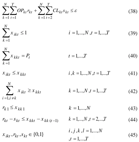
The objective function (1) maximizes the total covered flows during the planning horizon. The objective function (2) minimizes the total cost of establishing and closing hubs during the planning horizon. Constraints set (3) ensure that in each period, each non-hub node can be allocated to at most one hub. Constraints set (4) show the number of hubs which are going to be operated in each period. Constraints set (5) state that in each period, node i can be allocated to node k, if node k is served as a hub. Constraints set (6) show that in each period, the path i → k → l → j will be established where node i is allocated to hub k and node j is allocated to hub l. Constraints set (7) ensure that in each period, the path i → k → l → j is established, where traveling time is less than the coverage radius of β. Constraints set (8) and (9) indicate the possibility of creating and closing hubs over different periods. It is possible to close a hub if it had been located in previous periods and it can be opened if it had not been established in the previous periods. Constraints set (10) represent the type of decision variables. In the next section, the method of solving the proposed model is investigated.

3. SOLUTION APPROACH

Epsilon constraint method is one of the most appropriate solution methods for multi-objective programming models and is one of the recommended ways when there is no access to the decis ion makers (DM) [17]. In this method, after selecting one of the objectives as the primary objective function, others are moved into the problem constraints and an upper or lower limit (ε) is considered for them. As a result, the multi-objective problem is converted into a single-objective problem and Pareto solutions can be determined by assigning different values to Epsilon [18]. Consider the multi-objective programming problem (11) which consists of m different objectives and S represents the feasible region [17].

(11)





/ ( ), ( ),..., ( )

. .

m

Max Min f x f x f x s t xS

By choosing k (k∈ {1,...,m}) as the primary objective, the other objectives are moved to the constraints.

(12)

/ ( )

. . k

Max Min f x s t xS

(13)





( ) 1,..., ,

i i

f x  i m ik for max objectives

(14)





( ) 1,..., ,

j j

3. 1. ε-constraint Method To implement the ε -constraint method in the proposed BOMMHCP model, two single-objective problems are considered as follows.

Problem 1:

The objective function (1)

s.t.

Constraints (3)-(10)

1 1 1 2

N T N T

kt kt kt kt

k t k t

OP r CL s 

   

 





The parameter Obj 1 is equal to value of the optimal objective function of problem 1.

Problem 2:

The objective function (2)

s.t.

Constraints (3)-(10)

1 1, 1 1 1

1

N N N N T

ijt ijklt i j i k l t

W y Obj

     



  

The following steps are implemented to obtain the set of Pareto optimal solutions:

Step 1: Set the Pareto optimal solutions to the empty and the ε value to infinity.

Step 2: Solve Problem 1. If the problem has an optimal solution, then set the Obj 1 and go to step 3. Otherwise, stop.

Step 3: Solve Problem 2. Put Obj 2 equal to the value of the optimal objective function and go to step 4. Step 4: Add the solution (Obj 1, Obj 2) to the Pareto optimal solutions and go to step 5.

Step 5: Set the value of ε to (Obj 2-1) and go to step 2. Problem 1 in ε-constraint MILP model of BOMMHCP is computationally intractable such that even small-size examples cannot be solved optimally in a reasonable runtime using a commercial solver. Accordingly, we proposed a valid inequality to accelerate the solving process of the problem. Since BOMMHCP is a single allocation model and each non-hub node can be connected to at most one hub, then at most one path would be existed to transfer the flow between each O/D pair. Therefore, valid inequality can be stated as follows:

1 1 1

N N ijklt k l

y

 





By increasing the number of network nodes and periods, Problem 1 will be intractable due to the existence of

many binary variables and constraints and addition of valid inequality (17) does not help either to solve the problem in a reasonable time. As a result, to accelerate the solution process, the Benders decomposition algorithm will be developed in the following section.

3. 2. Benders Decomposition (BD) BD is a

classical solution approach that was initially introduced in 1962 by Benders to solve the NP-hard Mixed Integer Programming (MIP) problems. In this algorithm, the MIP model is decomposed into two s maller problems: the Master Problem (MP) and the Sub-problem (SP). The MP only contains integer variables and the SP includes continuous variables of the original problem. The MP and SP are iteratively solved to produce lower bound (LB) and upper bound (UB) for optimal objective value. Then, by the convergence of LB and UB, the optimal solution is found. To illustrate the Benders decomposition algorithm, consider the following MIP model [19]:

:min

0

T T

P C x f y Ax By b Dy d y Z x



     

₍₁₈₎

Or equivalently,

:min T ( ) MP f y y

Dy d y Z





  

(19)

where,

: ( ) min

0

T

SP y C x Ax b By x

 

  

(20)

By fixing y to the feasible values (y ), the dual of sub-problem (DSP) is shown as follows:

: max ( )

0

T

T

DSP b By u A u c

u

  

(21)

By obtaining the optimal values of u (u ) the relaxed master problem is shown as follows:

: min

( )

( ) 0

T T

T

RMP Z

Z b By u f y u P

b By u u R

Dy d y Z

              

 

(22)

defined by the constraint sets of DSP model (). The classical BD algorithm is operated as follows for the minimizat ion problem [19]:

y := initial feasible integer solution :

LB   and UB: 

while UBLB (δ is the user-defined optimality gap) do

solve the DSP ()

if the DS P () Unbounded then

Get unbounded ray u and Add the cut (bBy)Tu 0 to the RM P ()

else

Get the extreme point u and Add the cut

( )T T

Z  b By u f y to the RM P ()

UB: min





solve the RM P ()

Z: min{ Z cuts y| , Z}and LB:Z

end while

In the following, we develop BD for the ε-constraint model of BOMMHCP.

3. 2. 1. The Sub-Problem The SP for the fixed

integer variable x x , is created as follows:

1 1, 1 1 1

N N N N T

ijt ijklt i j i k l t

Min W y

     



  

s.t.

2yijklt xiktxjlt

, , 1,..., , 1,...,

i j k l N t T

 

 (24)

(D_ik D_klD_lj)y_ijklt , , 1,...,

, 1,...,

i j k l N t T    (25) 1 1 1 N N ijklt k l y   



{0,1} ijklt

y  , , , 1,...,

, 1,...,

i j k l N t T



 (27)

BD uses the results of the dual SP solutions to create cutting constraints in each iteration. SP has binary variables and its dual representation is not possible. So, firstly, the structure of SP model is changed in order to transform it into a model with continuous variables. So:

1 1, 1 1 1

N N N N T

ijt ijklt ijklt i j i k l t

Min W A y

     



  

s.t.

ijklt kkt

y x i j k l, , 1,...,N t, 1,...,T ₍₂₉₎

ijklt llt

y x ij k l, , 1,...,N t, 1,...,T (30)

1 1 1 N N ijklt k l y   



0y_ijklt 1 i j k l, , , 1,...,N t, 1,...,T (32)

The parameter A_ijklt is used to specify the feasible paths with respect to the coverage radius, as follows:

1 ( )

0

ik kl lj ijklt ijklt

if D D D y A else          

3. 2. 2. The Dual of Sub-Problem Given the dual

variables e_ijklt for constraints set (29), f_ijklt for constraints set (30) and g_ijtfor constraints (31), the dual

of SP (DSP) is created as follows:

1 1, 1 1 1

1 1, 1 1 1

1 1, 1

N N N N T

kkt ijklt i j i k l t

N N N N T

llt ijklt i j i k l t

N N T

ijt i j i t

Max x e

x f g                    

  

  

  

e_ijklt f_ijklt g_ijt  W_ijtA_ijklt , , 1,...,

, 1,...,

i j k l N t T

 

 (4)

eijklt,fijklt,gijt 0

, , , 1,..., , 1,...,

i j k l N t T



 (5)

Constraints set (4) are related to the primal variable ijklt

y .

3. 2. 3. The Relaxed Master Problem (RMP) SP

always has a feasible and finite optimal solution. Therefore, by dual theory, DSP has an optimal finite solution (e_ijklt,f_ijklt,g_ijt ). Thus, by the principle of

weak duality, the optimality Benders cut is obtained as constraint (37). As a result, the RMP is created as follows:

Min Z (36)

s.t.

1 1, 1 1 1

1 1, 1 1 1

1 1, 1

N N N N T

kkt ijklt i j i k l t

N N N N T

llt ijklt i j i k l t

N N T

ijt i j i t

Z x e

1 1 1 2

N T N T

kt kt kt kt

k t k t

OP r CL s 

   

 





1

1 N

ikt k

x

 



1

N

kkt t k

x P

 



ikt kkt

x x i k, 1,..., ,N t1,...,T (41)

1,

N

ikt kkt i i k

x x

  



1 1

k kk

r x k 1,...,N (43)

( 1)

kt kt kkt kk t

r s x x _ k1,..., ,N t2,...,T (44)

, , {0,1}

ikt kt kt

x r s  , , , 1,...,

, 1,...,

i j k l N t T



 (45)

3. 2. 4. Accelerating the Proposed BD In some

cases, direct use of classic BD may not result in a significant reduction in solution runtime. Some of the main reasons for the slow convergence rate of the classical BD are: (1) solving the excessive numbers of RMPs and SPs, and (2) the low quality of the cuts created in each iteration. Therefore, various methods and techniques have been developed to increase the convergence speed of the BD [20].

In early runs of BD, it was observed that there was a low convergence rate at the lower bound of the objective function (RMP problem). Therefore, to increase the efficiency and speed of BD, the cutting constraints set (46)-(47) are added to RMP problem. These constraints limit the maximum flow through the network.

1

1

N

ijt ijklt ikt jlt k

h A x x







, 1,...,

i j l N t T



 (46)

1 1, 1

N N T

ijt ijt

i j i t

Z W h

   

 

  

4. COMPUTATIONAL RESULTS

Experiments were conducted to assess the performance of the valid inequality and proposed Benders decomposition approach. In the following, we will explain the data generation approach and analyze the obtained results.

4. 1. Data Generation The well known standard

benchmark that is refers to data obtained from the Civil Aeronautics Board of the United States of America (CAB dataset [21]), is used for evaluating BOMMHCP model. Since the CAB dataset is not provided for multi-period problems. Therefore, according to Alumur et al. [22], flows in the CAB dataset are considered for the first period only. Also, for following periods, it is obtained from the multiplication of the flows of the previous period by a random number from the uniform interval (0.9, 1.2). The cost of establishing and closing hubs has been generated according to Gelareh et al. [23]. Moreover, the cost of establishing the hub for the first period is randomly generated from the interval (500,700). Likewise, for following periods, it is obtained from the multiplication of the establishment costs of the previous period by a random nu mber from the uniform interval (1, 1.05). Additionally, the cost of closing the hub for the first period is randomly generated from the interval (200,300) and for following periods, it is obtained from the multiplication of the closing costs of the previous period by a random number from the uniform interval (1, 1.05). Different values for discount factor and coverage radius are considered according to the article by Silva and Cunha [24]. The various values of the parameters are shown in

TABLE .

4. 2. Results Analysis The GAMS software

(version 24.9.1) and CPLEX solvers (version 12.7.1) were used for solving ε-constraint MILP model of BOMMHCP and the proposed BD algorithm. The software runs on a 4 GHz Intel processor (Intel Core i7-6700k) and 32GB of RAM. A time limit of 7200 and 3600 seconds was considered for the implementation of ε-constraint MILP model with valid inequality and BD algorithm, respectively. In continue, we will explain the results from various aspects.

TABLE 1.Parameter Values forBOM M HCP

Parameter Value s

N 10,15,20,25

P 2,3,4,5

ijt

W

( 1)

[0.9,1.2] 1

1

ij t

CAB da

W U t

taset t

  



kt

OP

( 1)

1 [500, 700]

[1.05,1.1] 1

k t

t U

OP _ U t



 

kt

CL

( 1)

2 [200,300]

[1.05,1.1] 2

k t

t U

CL _ U t



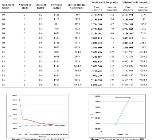
4. 2. 1. Performance of The Valid Inequality Different problems with 10 and 15 nodes were solved to illustrate the efficiency of valid inequality and the results are presented in Table 2. The stars (*) indicate that the optimal solution has been achieved. As it is evident, the optimal solution is obtained by applying the valid inequality (17) for all sample issues, while without considering the inequality, only the optimal solution to the problems with ten nodes is obtained. Also, the results confirm the high performance of a valid inequality in terms of runtime and show a significant decrease.

4. 2. 2. Evaluation of Speeding Up The BD In

this paper, we proposed a modification to speeding up the classical BD algorithm. The computational results are presented in Figures 1 and 2. Several experiments have been conducted to verify the effectiveness of correction. As an example, the N10P2T3α0.2R1425 problem (problem with ten nodes, two hubs, three periods, α=0.2 and the coverage radius of 1425) is solved by the classical BD and improved BD. The results show that the classical BD converges in iteration 39 (Figure 1Figure ), while, the improved BD converges in two iterations (Figure 2).

TABLE 2. Results of adding Valid Inequality

Number of Node s

Numbe r of Hubs

Discount Factor

C ove rage Radius

Epsilon (Budge t C onstraint)

W ith Valid Ine quality Without Valid Inequality

Flow Objective

Runtime (seconds)

Flow Objective

Runtime (seconds)

10 2 0.2 1425 1599 3,174,972* 3.2 3,174,972* 77.6

10 3 0.2 1117 2433 3,139,640* _{3.0 3,139,640}* ₁₉₃

10 4 0.2 811 3273 2,794,350* 4.7 2,794,350* 185.2

10 5 0.2 736 4134 2,733,823* _{7.9 2,733,823}* _147.3

10 2 0.6 1671 1599 3,136,301* 4.0 3,136,301* 73.9

10 3 0.6 1387 2433 3,091,015* _{2.6 3,091,015}* _179.7

10 4 0.6 1148 3273 3,021,212* _{1.7 3,021,212}* _281.4

10 5 0.6 1079 4134 2,896,000* 1.9 2,896,000* 138.7

15 2 0.2 2004 1564.5 7,470,656* _{275 7,407,953 4634.4}

15 3 0.2 1638 2349 7,341,687* 183 7,142,206 7203.2

15 4 0.2 1324 3138 7,051,643* _{278 6,912,159 7203.4}

15 5 0.2 1149 3964.5 7,075,740* 115 6,706,032 7203.9

15 2 0.6 2103 1564.5 7,179,215* _{340 7,133,948 7203.3}

15 3 0.6 1844 2349 7,073,270* 513 6,933,837 7203.5

15 4 0.6 1756 3138 7,146,254* 125 6,589,729 7203.2

15 5 0.6 1560 3964.5 6,871,335* 134 6,430,333 7203.8

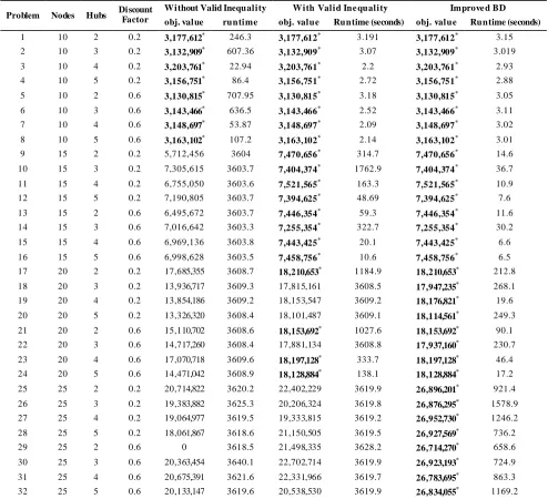
4. 2. 3. Verifying and Validating the BD

Algorithm Several examples were solved to confirm

the efficacy of the improved BD algorithm. The obtained results are presented in Table 3. The stars (*) indicate that the optimal solution has been achieved.

The results demonstrated that the performance of the ε-constraint MILP models with and without valid inequality and the Improved BD algorithm are similar and they reach to the optimal solution for all instances with ten nodes in less than 3600 seconds. However, in all instances with 15 nodes, only ε-constraint MILP models with valid inequality and the improved BD

algorithm performed similarly, while ε-constraint MILP models without valid inequality was not capable of solving the samples at the proposed runtime limitation and made even worse objective values . In addition, the results obtained from instances with 20 and 25 nodes demonstrated that the proposed BD algorithm performed better than the others and it had less runtime, and more appropriate solutions were obtained. The comparison of solution times and objective values are shown in Figures 3 and 4, respectively.

TABLE 1.Results of improved BD

Problem Nodes Hubs Discount _Factor Without Valid Inequality W ith Valid Ine quality Improve d BD

obj. value runtime obj. value Runtime (seconds) obj. value Runtime (seconds)

1 10 2 0.2 3,177,612* _{246.3 3,177,612}* _{3.191 3,177,612}* _3.15

2 10 3 0.2 3,132,909* 607.36 3,132,909* 3.07 3,132,909* 3.019

3 10 4 0.2 3,203,761* 22.94 3,203,761* 2.2 3,203,761* 2.93

4 10 5 0.2 3,156,751* 86.4 3,156,751* 2.72 3,156,751* 2.88

5 10 2 0.6 3,130,815* _{707.95 3,130,815}* _{3.18 3,130,815}* _3.05

6 10 3 0.6 3,143,466* 636.5 3,143,466* 2.52 3,143,466* 3.11

7 10 4 0.6 3,148,697* 53.87 3,148,697* 2.09 3,148,697* 3.02

8 10 5 0.6 3,163,102* 107.2 3,163,102* 2.14 3,163,102* 3.01

9 15 2 0.2 5,712,456 3604 7,470,656* _{314.7 7,470,656}* _14.6

10 15 3 0.2 7,305,615 3603.7 7,404,374* _{1762.9 7,404,374}* _36.7

11 15 4 0.2 6,755,050 3603.6 7,521,565* 163.3 7,521,565* 10.9 12 15 5 0.2 7,190,805 3603.7 7,394,625* 48.69 7,394,625* 7.6 13 15 2 0.6 6,495,672 3603.7 7,446,354* 59.3 7,446,354* 11.6 14 15 3 0.6 7,016,642 3603.3 7,255,354* _{322.7 7,255,354}* _30.2

15 15 4 0.6 6,969,136 3603.8 7,443,425* _{20.1 7,443,425}* _6.6

16 15 5 0.6 6,998,628 3603.5 7,458,756* 10.6 7,458,756* 6.5 17 20 2 0.2 17,685,355 3608.7 18,210,653* 1184.9 18,210,653* 212.8 18 20 3 0.2 13,936,717 3609.3 17,815,161 3608.5 17,947,235* _268.1

19 20 4 0.2 13,854,186 3609.2 18,153,547 3609.2 18,176,821* _19.6

20 20 5 0.2 13,326,320 3608.4 18,101,487 3609.1 18,114,561* 249.3 21 20 2 0.6 15,110,702 3608.6 18,153,692* 1027.6 18,153,692* 90.1 22 20 3 0.6 14,717,260 3608.4 17,881,134 3608.8 17,937,160* 230.7 23 20 4 0.6 17,070,718 3609.6 18,197,128* _{333.7 18,197,128}* _46.4

24 20 5 0.6 14,471,042 3608.9 18,128,884* _{138.1 18,128,884}* _17.2

25 25 2 0.2 20,714,822 3620.2 22,402,229 3619.9 26,896,201* 921.4 26 25 3 0.2 19,383,882 3625.3 20,206,324 3619.8 26,876,295* 1578.9 27 25 4 0.2 19,064,977 3619.5 19,333,815 3619.2 26,952,730* 1246.2 28 25 5 0.2 18,061,867 3618.6 21,150,505 3619.5 26,927,569* _736.2

29 25 2 0.6 0 3618.5 21,498,335 3628.2 26,714,270* _658.6

Figure 3. The comparison of the solution time of improved BD versus 𝛆-constraint M ILP model

Figure 4. The comparison of the objective value of improved BD versus 𝛆-constraint M ILP model

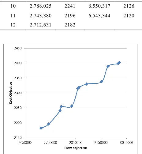
4. 2. 4. Pareto Optimal Solutions Two sample

problems have been solved to illustrate Pareto's optimal solutions in 𝛆-constraint method, including the problem with ten nodes, four hubs, three time periods and discount factor of 0.6 (N10P4T3α0.6) and the problem with 15 nodes, four hubs, three time periods and discount factor of 0.6 (N15P4T3α0.6). Results are shown in Table 4, Figures 5 and 6.

TABLE 4. Pareto optimal solutions for problems with 10 and 15 nodes

Solution Numbers

N10P4T3α0.6 N15P4T3α0.6

Flow O bj. C ost Obj. Flow O bj. C ost Obj.

1 3,021,212 2402 7,146,254 2430

2 3,017,047 2398 7,124,188 2396

3 2,977,080 2389 7,096,680 2290

4 2,951,872 2338 7,083,419 2288

5 2,892,576 2330 7,074,650 2260

6 2,862,641 2319 7,015,516 2225

7 2,858,476 2315 6,884,141 2204

8 2,834,144 2256 6,721,777 2179

9 2,793,301 2255 6,702,545 2151

10 2,788,025 2241 6,550,317 2126

11 2,743,380 2196 6,543,344 2120

12 2,712,631 2182

Figure 5. Optimal Pareto Front for N10P4T3α0.6

Figure 1. Optimal Pareto Front for N15P4T3α0.6

Hub node

Hub arc Access arc

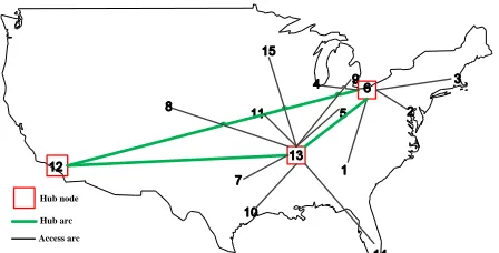
Figure 7. Network structure for N15P3T3 in the first period

Hub node

Hub arc Access arc

Figure 8. Network structure for N15P3T3 in the Second period

Hub node

Hub arc Access arc

Figure 9. Network structure for N15P3T3 in the third period

5. CONCLUSIONS

In this paper, by considering the periodic changes in O/D flows and the costs of establishing and closing hubs, a mathematical model was proposed for a bi-objective multi-period maximal hub covering problem. Furthermore, the ε-constraint method was used to solve the proposed model. Given that the single-objective problem found in the ε-constraint method is computationally intractable, we added a new valid inequality and also developed the BD algorithm to accelerate the solution process. Results showed that the proposed BD has a high performance in terms of runtime and optimal attainment.

This work covers the application of HLPs in periodic variation of parameters. However, there are

still issues for development. One of them includes taking into account stochastic parameters (such as O/D flows, traveling time and costs) along with periodic parameters to increase the efficiency of the BOMMHCP model when the decision parameters are changing. Meanwhile, it is useful to extend the proposed model by considering other constraints of the real world, including the amount of available budget and capacity constraint in the network.

6. REFERENCES

1. Contreras, I., Hub location problems, in Location science, G. Laporte, S. Nickel, and F. Saldanha da Gama, Editors. 2015, Springer International Publishing: Cham. 311-344. 2. Campbell, J.F., "Integer programming formulations of discrete

hub location problems", European Journal of Operational Research, Vol. 72, No. 2, (1994), 387-405.

3. Karimi, H. and Bashiri, M., "Hub covering location problems with different coverage types", Scientia Iranica, Vol. 18, No. 6, (2011), 1571-1578.

4. Hwang, Y.H. and Lee, Y.H., "Uncapacitated single allocation p-hub maximal covering problem", Computers & Industrial Engineering, Vol. 63, No. 2, (2012), 382-389.

5. Jabalameli, M.S., Barzinpour, F., Saboury, A. and Ghaffari-Nasab, N., "A simulated annealing-based heuristic for the single allocation maximal covering hub location problem",

International Journal of Metaheuristics, Vol. 2, No. 1, (2012), 15-37.

6. Ebrahimi-zade, A., Sadegheih, A. and Lotfi, M.M., "A modified nsga-ii solution for a new multi-objective hub maximal covering problem under uncertain shipments",

Journal of Industrial Engineering International, Vol. 10, No. 4, (2014), 185-197.

7. Pasandideh, S.H.R., Niaki, S.T .A. and Sheikhi, M., "A bi-objective hub maximal covering location problem considering time-dependent reliability and the second type of coverage",

International Journal of Management Science and Engineering Management, Vol. 11, No. 4, (2015), 195-202. 8. Bashiri, M. and Rezanezhad, M., "A reliable multi-objective

p-hub covering location problem considering of p-hubs capabilities", International Journal of Engineering-Transactions B: Applications, Vol. 28, No. 5, (2015), 717-729.

9. Karimi, H., Bashiri, M. and Nickel, S., "Capacitated single allocation p-hub covering problem in mult i-modal network using tabu search", International Journal of Engineering-Transactions C: Aspects, Vol. 29, No. 6, (2016), 797-808. 10. Ebrahimi-zade, A., Sadegheih, A. and Lotfi, M.M., "Fuzzy multi-objective linear programming for a stochastic hub maximal covering problem with uncertain shipments",

International Journal of Industrial and Systems Engineering, Vol. 23, No. 4, (2016), 482-499.

11. Janković, O. and Stanimirović, Z., "A general variable neighborhood search for solving the uncapacitated r-allocation p-hub maximal covering problem", Electronic Notes in Discrete Mathematics, Vol. 58, (2017), 23-30.

13. Madani, S.R., Shahandeh Nookabadi, A. and Hejazi, S.R., "A bi-objective, reliable single allocation p-hub maximal covering location problem: Mathematical formulation and solution approach", Journal of Air Transport Management, Vol. 68, (2018), 118-136.

14. Gelareh, S., "Hub location models in public transportation planning", Kaiserslaut ern University of T echnology, Ph.D, T hesis (2008),

15. Ebrahimi-zade, A., Hosseini-Nasab, H., zare-mehrjerdi, Y. and Zahmatkesh, A., "Multi-period hub set covering problems with flexible radius: A modified genetic solution", Applied Mathematical Modelling, Vol. 40, No. 4, (2016), 2968-2982. 16. Campbell, J.F. and O'Kelly, M.E., "T wenty-five years of hub location research", Transportation Science, Vol. 46, No. 2, (2012), 153-169.

17. Balaman, Ş.Y., Matopoulos, A., Wright, D.G. and Scott, J., "Integrated optimization of sustainable supply chains and transportation networks for multi technology bio-based production: A decision support system based on fuzzy ε-constraint method", Journal of Cleaner Production, Vol. 172, (2018), 2594-2617.

18. Yu, H. and Solvang, W.D., "An improved multi-objective programming with augmented ε-constraint method for hazardous waste location-routing problems", International

Journal of Environmental Research and Public Health, Vol. 13, No. 6, (2016), DOI: 10.3390/ijerph13060548. 19. Emami, S., Moslehi, G. and Sabbagh, M., "A benders

decomposition approach for order acceptance and scheduling problem: A robust optimization approach", Computational and Applied Mathematics, Vol. 36, No. 4, (2017), 1471 -1515. 20. Saharidis , K.D., Minoux , M. and Ierapetritou , G., "Accelerating benders method using covering cut bundle generation", International Transactions in Operational Research, Vol. 17, No. 2, (2010), 221-237.

21. O'Kelly, M.E., "A quadratic integer program for the location of interacting hub facilities", European Journal of Operational Research, Vol. 32, No. 3, (1987), 393-404.

22. Alumur, S.A., Nickel, S., Saldanha-da-Gama, F. and Seçerdin, Y., "Multi-period hub network design problems with modular capacities", Annals of Operations Research, Vol. 246, No. 1, (2016), 289-312.

23. Gelareh, S., Neamatian Monemi, R. and Nickel, S., "Multi-period hub location problems in transportation",

Transportation Research Part E: Logistics and Transportation Review, Vol. 75, (2015), 67-94.

24. Silva, M.R. and Cunha, C.B., "A tabu search heuristic for the uncapacitated single allocation p-hub maximal covering problem", European Journal of Operational Research, Vol. 262, No. 3, (2017), 954-965.

Mathematical Model for Bi-objective Maximal Hub Covering Problem with Periodic

Variations of Parameters

Y. Khosravian Ghadikolaei, A. Shahandeh Nookabadi, G. Moslehi

Department of Industrial and Systems Engineering, Isfahan University of Technology, Isfahan, Iran

P A P E R I N F O

Paper history: Received 04 March 2019

Received in revised form 30 April 2019 Accepted 03 May 2019

Keywords:

Maximal Hub Covering Dynamic Hub Location Multi-period Hub Location ε-constraint Method Benders Decomposition هدیکچ رثکادح هلأسم باه ششوپ زا یکی م ئاس گنارب شلاچ ل زی قحت رد قی لمع تای همانرب و ر یزی لقن و لمح هدوب

نآ فده هک

نتفای هب ناکم هنی ی هعومجم ا ی باه زا ارب اه ی سر ندی رج رثکادح هب نای

رد کی ئاجنآ زا .تسا هکبش ی هک رد ند یای عقاو ی اهرتماراپ ی لصا ی هلأسم رج دننام ای ن و أدبم نیب زه ،دصقم نی ه هرود روط هب رفس نامز و اه ا ی غت ریی م ی رد ،دننک ههجاوم اب نآ یم اه هب یتادیهمت تسیاب دنوش هتفرگ راک

ا رد . نی ارب ،هلاقم ی غت اب هلباقم تاریی هرود ا ی ،اهرتماراپ کی ر لدم یضای ود

ارب هفده ی هلاسم رثکادح ششوپ صیصخت اب ایوپ باه یکت

دش هئارا ه .تسا باوج هب یسرتسد یارب زا هریچان یاه

ور درکی دودحم .تسا هدش هدافتسا نولیسپا تی ا هب هجوت اب

هکنی هلئسم ی فده کت رد هدش داجیا ه شور نولیسپا تیدودحم رظن زا تابساحم ی تسا هدیچیپ روگلا ، متی زجت هی ی زردنب هفاضا اب ندومن تلاداعمان ارب ربتعم ی شخب تعرس ندی آرف هب دنی لح اد هعسوت هد اهن رد .تسا هدش ،تی

پ شور یداهنشی زا هدافتسا اب هداد هعومجم CAB هدش ارجا اتن و جی هب هدمآ تسد ناشن رظن زا یداهنشیپ متیروگلا ییاراک هدنهد هب

یگنی ارجا نامز و یم دشاب

.