© Shiraz University
TARGET TRACKING AND RECEIVER PLACEMENT
IN MIMO DVB-T BASED PCL
*M. RADMARD
**AND M. M. NAYEBI
Sharif University of Technology, Tehran, I. R. of Iran Email: [email protected]
Abstract– Recently many studies have been done on different issues of using multiple antennas at transmit and receive sides of a radar system in a MIMO (Multiple Input Multiple Output) configuration. In addition, for the purpose of electronic warfare, the utilization of available signals of the environment to detect the targets has gained considerable attention in recent years. Such passive radars use the transmitter of other purposes (e.g. the GSM or television stations) as their noncooperative transmitter. Moreover, the idea of using multiple of such illuminators to get the advantages of MIMO technology, besides the advantages of passive illumination, is new and attractive. An excellent candidate of such configuration is a DVB-T SFN (single frequency network). However, various obstacles and considerations appear when working with a MIMO DVB-T based passive radar system. In this paper, we consider two such problems: tracking multiple targets and choosing appropriate positions for the receive antennas in the surveillance region. First, based on the previously developed schemes to associate the receive data to the transmitters and targets, we propose a tracking algorithm to extract the true targets from the candidate targets. Then, we develop a procedure to place the receivers of such MIMO passive systems in such positions that result in better performance of the aforementioned association algorithm.
Keywords– MIMO, PCL, geometry optimization, receiver placement, tracking
1. INTRODUCTION
The emerging MIMO technology in the communications field [1] has attracted the radar researchers‟ attention, too. Recently there has been considerable study on the advantages of using multiple antennas at transmit and receive sides of a radar system (namely a MIMO radar) [2]. The antennas can be used in a widely separated manner or near each other like the traditional phased array. Based on this characteristic, MIMO radars are divided into two categories. In a widely separated antennas scheme [3] diversity gain [4,5] and high resolution target localization (spatial multiplexing gain)[2] can be obtained. Besides, improved parameter identifiability [6], direct applicability of adaptive arrays for detection and parameter estimation [7], and enhanced flexibility for transmit beam-pattern design [8,9] are achieved by the system with colocated antennas.
On the other hand, using the commercial transmitting stations already working in the environment as the noncooperative transmitter of the radar system makes the radar covert. Therefore this passive radar, or namely PCL (passive coherent location) is resilient to electronic countermeasures which use the signals emitted by the radar. The feasibility of different existing signals for the PCL applications has been previously investigated, for example, in the case of FM [10], analog TV [11,12], Digital TV (DTV) [13]-[15], satellite [16], and GSM [17,18] systems.
Received by the editors November 20, 2013; Accepted May 6, 2015.
In such passive system, two sets of antennas are used, one for receiving the direct signal from its main source (reference antenna) and another one for collecting reflections arriving from the targets (reflection antenna). Figure 1 depicts the structure of such system.
Fig. 1. Structure of a passive coherent location scheme
Here, detection is done through computation of CAF (Cross Ambiguity Function) given in (1) which shows how much correlation exists between reference and reflected signals. A CAF‟s peak in the range-Doppler board is representative of a target candidate:
∫ (1)
where is the received signal, is the reference signal, is the Doppler shift, is the delay shift, and is the integration interval.
New digital signals, such as Digital Audio/Video Broadcast (DAB/DVB), are excellent candidates for PCL purpose as they are widely available and can be easily decoded. Another remarkable property which makes them quite suitable for MIMO application is that DVB-T/DAB stations are broadcasting video/audio signals in a SFN (Single Frequency Network), in which multiple transmitters are transmitting the same signal in the same frequency. Thus the existing DVB-T transmitters of a SFN are good candidates for setting up a MIMO PCL. In addition, as shown in [14], the thumbtack ambiguity function of DVB-T makes it superior over other opportunistic signals considered to be used for PCL application.
However, since the DVB-T transmitters are working in a SFN (i.e. all of the transmitters are transmitting the same signal without any distinction), the data association problem would be an obstacle in such system. In other words, it is not apparent which transmitter and which target the peaks at the output of the CAF processor belong to. Some data association schemes were developed before to address this obstacle [19]-[22].
In addition, the issue of choosing proper positions for the antennas in order to improve the performance of the radar system is a topic that has been considered from different aspects in recent works. In this case, first, the goal should be cleared, e.g. improvement of the probability of detection [23]-[26], the detectors output SNR [27], the tracking performance, etc. It should be noted that in a MIMO PCL system, the transmitters are noncooperative, so that their positions are not under control. Therefore, only the receivers‟ positions are optimized.
targets in successive scans and deleting the false tracks. Then we consider the problem of choosing suitable positions for the receive antennas such that the performance of the aforementioned association algorithm is improved. In other words, in the second part, our aim is to optimize the geometry of antennas‟ positions such that the associated algorithms‟ performance is improved over the surveillance region.
In section 2, we describe how to extract the true targets from the candidate targets. Section 3 is devoted to the problem of finding proper positions for receive antennas. There, we will first consider positioning a single receiver. Then we will propose a procedure in order to extend the solution to the case of multiple receivers. Each case is followed by simulations. Finally, we conclude the paper in section 4.
2. REMOVING FALSE TARGETS THROUGH TRACKING
a) Problem formulation
Assume that there are an unknown number of targets, N, with illuminators of opportunity (e.g. broadcasting DVB-T signals in a Single Frequency Network) and receivers. For each receiver, the reflection antenna is assumed to be omnidirectional, collecting signals arriving from all directions. Each transmitter illuminates each object at each receiver with the probability (i.e., with probability of the echo from each object due to each transmitter would be detected at the receiver). We also assume a false alarm rate denoted by (i.e. with probability of false echoes appear at thereceiver). At the receiver side, after DPI cancellation, the signal is passed through a CAF processor to estimate delays and Doppler shifts of different echoes collected from the objects in the area. The reference signal is constructed from the direct signal received from the most powerful path. We use the term „measurement‟ for the information we obtain from each echo. Usually, each measurement consists of a delay and a Doppler shift. After constructing such measurements, two stages are involved implicitly in order to solve the association problem: the measurement-to-object association and then, the measurement-to-transmitter association. In [19, 20], for the case of MISO and MIMO respectively, algorithms are developed to assign these measurements of a single scan to the transmitters and targets. As a result, the locations of the targets can be determined. However, some of the resultant targets may be due to various forms of false associations, e.g. false alarm measurements mixed up with true measurements. Therefore, the outputs of such algorithm are candidate targets rather than true targets. Some rules have been proposed to decide whether a candidate target is a true one or not. For example, in the simulations of [28], it is suggested that a candidate target is a true one if it is detected by 4 or more sensors in a 7 sensor scenario with a probability of 0.997 and if there are only three sensors, a true target is detected by 2 or more sensors with a probability of 0.97. Then it is claimed that this assumption does not lead to a significant loss of accuracy. Here, our goal is to remove such uncertainty by using the previous data. In other words, we use the information of previous scans to determine whether a candidate is a true target or not. Our method is to track the candidate targets. As a result, a false target, obtained because of false association, disappears through successive scans. Here, we use the assumption of linearity for the targets‟ motion, so that it allows us to use the Kalman filter [29].
b) Kalman filtering
In order to use the Kalman filter to estimate the internal state of a process given only a sequence of noisy observations, we must model the process in accordance with the framework of the Kalman filter. In other words, first, we should specify the following matrices: , the state-transition model; , the observation model. The Kalman filter model assumes the true state at time is evolved from the state at
according to
(2)
is the state transition model;
is the process noise, which is assumed to have a zero mean normal distribution with covariance .
At time k a measurement of the true state is made according to
(3)
where is the observation model which maps the true state space into the observed space and is the observation noise which is assumed to be zero mean Gaussian white noise with covariance .
The algorithm works in a two-step process. In the prediction step, the Kalman filter produces estimates of the current state variables, along with their uncertainties, using the previous observations. Once the outcome of the next measurement (corrupted with noise) is observed, these estimates are updated using a weighted average, with more weight being given to estimates with higher certainty. Here, we do not explain the mathematical details of its algorithm (For more details see [29]). In our problem, the parameters of the filter are as follows,
includes the position and velocity ̇ ̇ of the target, i.e. ̇ ̇ .
[
]
[ ]
where is the scan duration.
Finally, it should be noted that, for the tracking system to perform properly the most likely measured potential target location should be used to update the target‟s state estimator. Here, we use the “Nearest Neighbor” algorithm, which updates the tracking filter with the measurement closest to the predicted state.
c) Forming the tracks
Two kinds of tracks are defined: 1) tentative tracks and 2) confirmed tracks. Initially, by receiving the measurements a tentative track is constructed which is an indicator of a possible target. Subsequently, by receiving and associating more measurements to these tracks, the tentative tracks are promoted as confirmed tracks, which represent the targets. Otherwise, if an insufficient number of measurements are associated to a tentative track, it is deleted. In addition, if no measurement is associated to a confirmed track for a long time it is deleted, which means that the respective target is no longer present. It should be noted that tentative tracks are formed with fewer initial measurement associations than that of confirmed tracks. The logic used for forming the tracks is as follows,
1. Out of successive measurements, if at least measurements are associated together, then form a track and tag it tentative; otherwise, do nothing.
2. Out of successive measurements, if at least measurements are associated to the track, then promote it as confirmed; otherwise, delete it.
3. Out of successive measurements, if at least measurements are associated to the track, then do nothing; otherwise, delete it.
d) Simulations
(5.01,-5.85) km at constant velocity of 0.36 Mach. The region of interest is a square region of . Three DVB-T transmitters and one receiver constitute our MIMO PCL system for surveillance of this region. The antennas‟ configuration is depicted in Fig. 2. In addition, are chosen for the rest of the simulations.
Fig. 2. The antennas‟ configuration of the tracking scenario
Furthermore, the parameters for forming the tracks are: tentative track formation logic is out of , tentative track maintenance logic is out of , and confirmed track deletion logic is out of . Finally, the initial values for the process noise covariance and the observation noise covariance are chosen as .
The result of applying the S-D association algorithm [19] to the bistatic ranges obtained from these targets at the receiver and the output of the proposed Kalman filter applied to these candidate targets are shown in Figs. 3a, 3b, respectively. As can be seen, in some scans the S-D algorithm has missed the targets. In addition, in some scans some false targets have been generated. After filtering, only the true targets have remained and other spurious data have been removed.
(a) (b)
Fig. 3. (a) The candidate targets, resulted from the S-D algorithm, (b) The result of Kalman filtering
their tracks. The result of applying the proposed Kalman filter is depicted in Fig. 4b. The filtering has, successfully, removed the false targets, and overcome the missed detections. The two deviations in the tracks, which seem to be the result of wrong localization by the S-D algorithm, are corrected in the subsequent scans.
(a) (b)
Fig. 4. Three targets moving with constant velocities, (a) The candidate targets, resulted from the S-D algorithm, (b) The result of Kalman filtering
Finally, we evaluate the performance of the proposed filter when the target has acceleration. The scenario includes two targets, moving parallel to each other. One is moving with constant velocity and the other with constant acceleration. The antennas‟ configuration is the same as Fig. 2. The first target wends its path from (-10, -10) km to (0, -10) km, at constant velocity of 0.62 Mach. The second target starts from (-10, -7) km at velocity of 0.31 Mach, and constant acceleration of 1.88 . Its end point is (-2.25, -7) km. The resulting candidate targets are shown in Fig. 5a. Figure 5b shows the result of tracking the targets by Kalman filtering. As can be seen, the result shows that the proposed design can also be applied to targets with non-constant velocities.
(a) (b)
Fig. 5. Two parallel targets, one with constant velocity and the other with constant acceleration, (a) The candidate targets, resulted from the S-D algorithm, (b)The result of Kalman filtering
Overall, the simulations‟ results show that the proposed algorithm gives satisfying results, when dealing with multiple targets, with different velocities and even with non-constant velocities.
3. RECEIVERS’ POSITIONING
the case of just one receiver. Then we will extend it to the MIMO case, so that multiple receive antennas are placed in the region of interest.
a) MISO configuration
1. Problem formulation and solution: In the case of a single receive antenna we need to define a proper criterion which would show the amount of appropriateness of each position when placing the receiver at that position. To do so, with respect to the S-D assignment algorithm‟s performance, we should consider the S-D algorithm in depth. Here, we explain the algorithm with a simple but sufficient interpretation for our purpose. For more details of this algorithm see [19].
Assume a region with M transmitters, a single receiver and an unknown number of targets. As mentioned before, the measurements at the receiver are the detected bistatic ranges. However, each measurement can belong to any transmitter and any target. If we assume that measurements are assigned to transmitters (i.e. we know the source of each measurement), we have M groups of measurements, each arriving from a different transmitter. We call this group configuration . The number of measurements in the ‟th group ( ) is denoted by , where denotes the measurement index. Each measurement ( ) is a representative of the distance from the transmitter to the target to the receiver:
(4)
where denotes the location of the transmitter of the ‟th group, is the receiver‟s position, is the target‟s location, and is the noise of the bistatic ranges.
The goal of S-D algorithm is to associate the observations from M groups, so that each M-tuple of measurements corresponds to a target. The likelihood of each M-tuple for representing a separate target can be calculated from this equation:
∏
(5)
where is the M-tuple of measurements and
√ ( )
(6)
The cost assigned to the M-tuple is given by
(7)
where denotes the likelihood of all measurements in being spurious (i.e. ).
It can be inferred that, if all measurements in a M-tuple belong to a true target, its cost is small. On the other hand, if the measurements are not assigned correctly to the right transmitter (or equivalently the right group) or to the right target, the cost of the corresponding M-tuple becomes high.
As explained previously, it can be inferred that the lower the right M-tuple‟s (i.e. the M-tuple corresponding to a true target) cost is, the better the S-D algorithm would work. In addition, the higher the wrong M-tuples‟ costs are, the more easily they are distinguished and removed by the S-D algorithm. The reason behind these two rules is that the algorithm is looking for M-tuples with less cost (or equivalently M-tuples more likely to be a target).
Therefore, by optimizing the antennas‟ geometry, we should make the right M-tuples‟ costs lower, and make the wrong M-tuples‟ costs higher. We use this fact and define our criterion for a specific geometry of transmitters, receiver and a target as:
∑ (8)
where is the number of possible M-tuples.
By this definition, for specific locations of the transmitters, the receiver and the target, more leads to better S-D algorithm‟s performance.
In order to compute the appropriateness of a specific receiver‟s location, we should consider the whole surveillance region for possible target positions. In other words, after positing the receiver at a specific position ( ), we consider each position of the region as a candidate of the target‟s position ( ). Then we compute for this specific receiver‟s and target‟s positions ( ). By changing the target‟s position ( ) over the whole region of interest, changes. Averaging over these s, which are resulted from all possible targets‟ positions( s) and a specific receiver‟s position ( ), helps us a gauge how suitable ( ) is for positioning the receiver. Finally, changing over the whole region of interest (i.e. considering all positions of the region as possible candidates for the receiver‟s location) and computing the average for each of them, we can choose the position with the highest average as the best position for the receiver ( ̂). In the following this procedure is explained through simulations.
2. An illustrative example: Consider two transmitters, one receiver, and a target as depicted in Fig. 6. The bistatic ranges detected at the receiver are listed in Table 1. All possible 2-tuples and their costs, computed from Eq. (7) are shown in Table 2. As expected, the right 2-tuple has the least cost. The resulting from this configuration, using Eq. (8), is .
Table 1. Bistatic ranges detected at the receiver
Source (TX#) bistatic range(km)
1 53.09
2 37.48
Table 2. Possible 2-tuples of Table 1
2-tuple Group 1 Group 2 cost
#1 dummy dummy 18.42
#2 dummy 53.09 8.48
#3 dummy 37.48 7.01 #4 53.09 dummy 7.35 #5 53.09 37.48 -2.59 #6 37.48 dummy 7.77
#7 37.48 53.09 -2.17
3. Simulations: For simulations, we consider the Imam Khomeini International Airport (IKIA) in Tehran, Iran, as the surveillance region. Our goal is to achieve the best radar coverage on IKIA by a MISO DVB-T based PCL system. This region is depicted from above in Fig. 7.
Fig. 7. Imam Khomeini International Airport (IKIA), Tehran, from above
Thus our region of interest for positing the receiver(s) is a rectangle of .
For more practical purposes, we define a priority function on the surveillance region. We assign a priority number (between 0 and 1) to every point of the region. This priority shows how important each point is from the surveillance point of view. The priority function we defined over IKIA is depicted in Fig. 8. From this figure it can be inferred that the priority function is defined such that the runway path is the most important district.
In order to address this issue (i.e. considering different priorities for different points), we compute the average for each receiver‟s position weighted by the priority function. In other words, in the stage of computing the average over all possible target‟s positions, first we weight with the priority function‟s values over the region and then get the average. Therefore, the weighted average , not the average itself, will be an indicator of how suitable a position is for positioning the receiver.
In our scenario there are two transmitters at (-1,1.13) km, (3.02,-0.71) km illuminating the airport. The goal is to posit a receiver in this region such that the mentioned S-D algorithm‟s performance over the region is improved with respect to the priority function of Fig. 8. Obviously this performance improvement is of utmost importance on the runway.
First, as a sample case, a display of values, weighted by the aforementioned priority function, for different target‟s positions with an arbitrary receiver‟s position is depicted in Fig. 9. The average of these values weighted by the priority function is a gauge of how much of the point (2.9,-1.1) km is suitable for being the receiver‟s position.
Fig. 9. Weighted values of over IKIA for a sample antennas configuration
The result of computing the weighted average for all possible receivers‟ positions is shown in Fig. 10. It can be seen that (-4.1,-0.38) km has the highest value and the receive antenna should be placed at that location.
Fig. 10. Weighted average for all possible receiver‟s positions
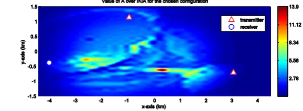
If we place the receiver at (-4.1,-0.38) km the weighted values of over IKIA obtained by such configuration will be as shown in Fig. 11.
b) MIMO configuration
1. Problem formulation and solution: In the previous section we proposed a method to posit the receiver of a MISO PCL such that the S-D assignment algorithm‟s performance is improved over the whole region of interest. Next, we consider the case of positing multiple receivers in order to achieve the same goal.
Similar to the case of MISO, for a MIMO configuration with specific locations of transmitters, receivers, the average value of over the whole region of interest (for all possible target positions) is a gauge of appropriateness from the S-D algorithm‟s point of view. In order to find the best configuration (or equivalently the best receivers‟ positions), we can test all possible positions for the receivers, as the procedure done in the MISO case. However, this procedure is almost practically impossible for the MIMO case, since the number of all possible MIMO configurations over the whole surveillance region is unacceptably high. In the following, we propose a procedure that is much more practical while maintaining almost the same efficiency. Here, first, the procedure is explained for the case of having less than four receivers. Then, the solution for the case of having four or more receivers is presented.
Instead of considering the whole region as candidate positions for positing the receivers, first, we divide the region into four equal rectangles and consider their centers as the only possible positions for positing the receivers. Then, we place the receivers at these rectangles‟ centers. It is obvious that by doing so, forming more than one configuration is possible. Next, for each possible configuration, we compute the average . The best average determines the best center points for positing the receivers.
After fixating the receivers at the appropriate centers, we aim to increase the positing accuracy by splitting the rectangles into smaller ones. Therefore, in the next stage, again, we divide the rectangles with the best centers into four smaller but equal rectangles. Then, for the receivers fixated at the bigger rectangles‟ centers, we test the four new centers of the new smaller rectangles. In this manner, the receivers‟ positing accuracy improves. We repeat this procedure of dividing the rectangles containing the receivers into smaller equal rectangles, successively, until no remarkable change is obtained in the receivers‟ positions.
It can be inferred that, the number of rectangles resulted from each splitting (e.g. four, as was the case up to here) should be more than the number of receivers. On the other hand, these rectangles should be equal. Therefore, if the number of receivers to be placed is given, one can easily determine the number of rectangles into which the primary rectangle should be split. For example, for five receivers, six or eight rectangles are appropriate, and more than that adds unnecessary computational burden.
In the following, an illustrative example is given to make this procedure clearer.
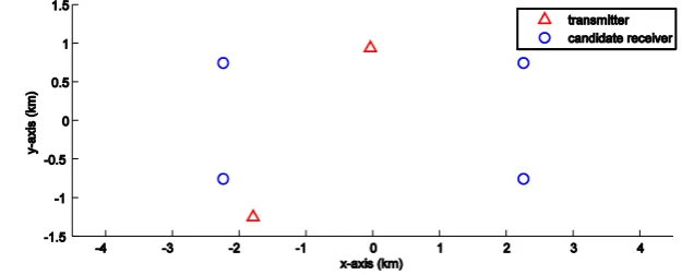
2. Simulations: Here, the region of interest is IKIA as the MISO case. Also, the priority function defined over the region is the same as Fig. 8. Our scenario consists of two transmitters at (-0.05, 0.93) km, (-1.8,-1.25) km and two receivers which should be placed at proper points. As described, first we consider the centers of the four rectangles as the only possible points for placing the receivers. These four points are shown in Fig. 12.
Then we form all possible configurations that can be assumed by placing the two receivers on these four points. For each configuration we compute our proposed criterion (i.e. the weighted average ). The results are shown in Table 3.
Table 3. Possible RXs‟ positions and their resulting performance
# RX 1 RX 2 Mean of weighted
1 (-2.25,0.75) (2.25,0.75) 5.32
2 (-2.25,-0.75) (2.25,-0.75) 5.43
3 (-2.25,0.75) (2.25,-0.75) 5.81
4 (-2.25,-0.75) (2.25,0.75) 5.19
5 (-2.25,-0.75) (-2.25,0.75) 5.97
6 (2.25,0.75) (2.25,-0.75) 6.15
It can be deduced that, in this stage the sixth case is the best of all. Figure 13 shows values of weighted average for this configuration.
Fig. 13. Weighted after placing the two receivers
As described before, in the next stage we divide the two rectangles containing the receivers into four smaller but equal rectangles and repeat finding the best configuration by changing the receivers‟ positions among these new rectangles‟ centers.
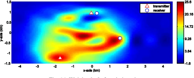
In order to get better accuracy, this procedure was repeated four more times. The result of this successive procedure was choosing (0.27,0.94) km , (1.58,-0.29) km as the positions to place the receivers. Figure 14 shows the value of weighted over IKIA area for the chosen configuration. Its weighted mean is 7.047, which shows its improvement after six iterations (compared with the sixth case of Table 3).
Fig. 14. Weighted after six iterations
In order to evaluate the proposed positioning procedure‟s performance, we compare the performance of the S-D algorithm to localize two targets at (2, 0) km, (-2, 0) km, for the two antennas‟ configurations:
1. the configuration resulted from the proposed algorithm, i.e. Fig. 14,
For the performance assessment, the following three parameters are measured for 100 runs of the S-D algorithm:
The percentage of correct measurement-to-transmitter association. This is an important parameter to see how correctly data is associated to its own group.
The average number of false targets appeared in an association procedure. If the measurements from different transmitters associated to a target are not really originated from a true target it will be categorized as a false target and be included in the total false alarm rate.
The probability of detection of each of the two true targets, represented.
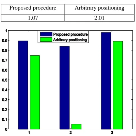
For the aforementioned scenario, the average number of false targets is shown in Table 4. The results for other evaluation parameters are depicted in Fig. 15.
Table 4. Average number of false targets
Proposed procedure Arbitrary positioning
1.07 2.01
Fig. 15. The test results for comparing the proposed positioning procedure and arbitrary positioning: 1. Percentage of correct measurement-to-transmitter association, 2. The probability of detection of the
first target, 3. The probability of detection of the second target
It can be inferred, from Fig. 15 and Table 4, that, in the arbitrary configuration, in spite of correct measurement-to-transmitter association, most of the time the first target is missed and instead, a false target is alarmed.
The evaluation results of Fig. 15 and Table 4, show the obvious superiority of the proposed procedure over arbitrarily positioning of the receivers.
4. CONCLUSION
In this paper, we addressed the target detection and tracking in MIMO PCL working in a SFN. First, we developed a method to extract the true targets from the candidate targets produced by the previously developed data association algorithms. Our method was to track the candidate targets to be able to distinguish between the true and false targets. Next, we considered the problem of choosing suitable positions for the receivers. We introduced a criterion which was a gauge of the appropriateness of a specific configuration of transmitters, receivers and a target. Finally, based on this criterion we proposed procedures to posit the receive antennas efficiently both in a MISO and MIMO configuration.
REFERENCES
1. Lozano, A. & Jindal, N. (2010). Transmit diversity vs. spatial multiplexing in modern MIMO systems. IEEE
Transactions on Wireless Communications, Vol. 9, pp. 186 –197.
2. Fishler, E., Haimovich, A., Blum, R., Chizhik, D., Cimini, L. & Valenzuela, R. (2004). MIMO radar: An idea
whose time has come. Proceedings of the IEEE Radar Conference, pp. 71–78.
3. Haimovich, A. M., Blum, R. S. & Cimini, L. J. (2007). MIMO radar with widely separated antenna. IEEE Signal
Processing Magazine, Vol. 25, No .1, pp. 116–129.
4. Lehmann, N. H., Fishler, E., Haimovich, A. M., Blum, R.S., Chizhik, D., Cimini, L. J. & Valenzuela, R. A.
(2007). Evaluation of transmit diversity in MIMO-radar direction finding. IEEE Transactions on Signal Processing, Vol. 55, No. 5, 2215–2225.
5. Fishler, E., Haimovich, A., Blum, R.S., Cimini Jr, L.J., Chizhik, D. & Valenzuela, R. A. (2006). Spatial diversity
in radars-models and detection performance. IEEE Transactions on Signal Processing, Vol. 54, No. 3, pp. 823–
838.
6. Li, J., Stoica, P., Xu, L. & Roberts, W. (2007). On parameter identifiability of MIMO radar. IEEE Signal Processing Letters, Vol. 14, No. 12, pp. 968–971.
7. Xu, L., Li, J. & Stoica, P. (2006). Radar imaging via adaptive MIMO techniques. Proc. 14'th European Signal Processing Conf., Florence, Italy.
8. Fuhrmann, D. R. & San Antonio, G. (2008). Transmit beamforming for MIMO radar systems using signal cross-correlation. IEEE Transactions on Aerospace and Electronic Systems, Vol. 44, No. 1, pp. 171–186.
9. Stoica, P., Li, J. & Xie, Y. (2007). On probing signal design for MIMO radar. IEEE Transactions on Signal Processing, Vol. 55, No. 8, pp. 4151–4161.
10. Howland, P. E., Maksimiuk, D. & Reitsma, G. (2005). FM radio based bistatic radar. IEE Proceedings-Radar, Sonar and Navigation. Vol. 152, pp. 107–115.
11. Griffiths, H. D. & Long, N. R. W. (2008). Television-based bistatic radar. IEE Proceedings F- Communications. Radar and Signal Processing, Vol. 133, No. 7, pp. 649–657.
12. Howland, P. E. (2002). Target tracking using television-based bistatic radar. In IEE Proceedings- Radar, Sonar and Navigation, Vol. 146, pp. 166–174.
13. Coleman, C. J., Watson, R. A. & Yardley, H. (2008). A practical bistatic passive radar system for use with DAB
and DRM illuminators. IEEE Radar Conference, pp. 1–6.
14. M. Radmard, M.H. Bastani, F. Behnia, and M.M. Nayebi. Feasibility analysis of utilizing the 8k mode DVB-T signal in passive radar applications. Scientia Iranica, Vol. 19, No. 6, pp. 1763–1770.
15. Saini, R. & Cherniakov, M. (2005). DTV signal ambiguity function analysis for radar application. In IEE Proceedings- Radar, Sonar and Navigation, Vol. 152, pp. 133–142.
16. Griffiths, H. D., Garnett, A. J., Baker, C. J. & Keaveney, S. (2002). Bistatic radar using satellite-borne
illuminators of opportunity. In International Radar Conference, pp. 276–279.
17. Tan, D. K. P., Sun, H., Lu, Y., Lesturgie, M. & Chan, H. L. (2005). Passive radar using Global System for
Mobile communication signal: theory, implementation and measurements. IEE Proceedings- Radar, Sonar and Navigation, Vol. 152, pp. 116–123.
18. Sun, H., Tan, D. K. P. & Lu, Y. (2008). Aircraft target measurements using A GSM-based passive radar. In IEEE Radar Conference, pp. 1–6.
19. Radmard, M., Karbasi, S. M., Khalaj, B. H. & Nayebi, M. M. (2012). Data association in multi-input
single-output passive coherent location schemes. IET Radar, Sonar & Navigation, Vol. 6, No. 3, pp. 149–156.
20. Radmard, M., Karbasi, S. M. & Nayebi, M. M. (2013). Data fusion in MIMO DVB-T -based passive coherent
location. IEEE Transactions on Aerospace and Electronic Systems, Vol. 49, No. 3, pp. 1725–1737.
21. Daun, M. & Koch, W. (2007). Multistatic target tracking for non-cooperative illuminating by DAB/DVB-T. In
22. Tharmarasa, R. Subramaniam, M., Nadarajah, N., Kirubarajan, T. & McDonald, M. (2012). Multitarget passive
coherent location with transmitter-origin and target-altitude uncertainties. IEEE Transactions on Aerospace and Electronic Systems, Vol. 48, No. 3, pp. 2530–2550.
23. Radmard, M., Khalaj, B. H., Chitgarha, M. M., Nazari Majd, M. & Nayebi, M. M. (2012). Receivers‟
Positioning in MIMO DVB-T Based Passive Coherent Location. IET Radar, Sonar & Navigation, Vol. 6, No. 7,
pp. 603–610.
24. Nazari Majd, M., Chitgarha, M. M., Radmard, M. & Nayebi, M. M. (2012). Probability of missed detection as a
criterion for receiver placement in MIMO PCL. In IEEE Radar Conference (RADAR), pp. 924–927.
25. Chitgarha, M. M., Nazari Majd, M., Radmard, M. & Nayebi, M. M. (2012). Choosing the position of the
receiver in a MISO passive radar system. 9’th European Radar Conference (EuRAD), pp. 318–321.
26. Chitgarha, M. M., Radmard, M., Nazari Majd, M. & Nayebi, M. M. (2014). Gradient descent-based power
allocation and receivers' positioning in MIMO radars. Iranian Journal of Science and Technology, Transactions of Electrical Engineering, Vol. 38, Vol. E2, pp. 111-203.
27. Chitgarha, M. M., Radmard, M., Nazari Majd, M., Khalaj, B. H. & Nayebi, M. M. (2012). The detector‟s output
SNR as a criterion for receiver placement in MIMO DVB-T based passive coherent location. 4th International
Congress on Ultra Modern Telecommunications and Control Systems and Workshops (ICUMT), pp. 431–435. 28. Deb, S., Yeddanapudi, M., Pattipati, K. & Bar-Shalom, Y. (1997). A generalized SD assignment algorithm for
multisensor-multitarget state estimation. IEEE Transactions on Aerospace and Electronic Systems, Vol. 33, No. 2, pp. 523–538.
29. Welch, G. & Bishop, G. (1995). An introduction to the Kalman filter.
30. Bar-Shalom, Y. & Li, X. R. (1995). Multitarget-multisensor tracking: principles and techniques. Storrs, CT: