Ma. Emilia Caballero & Lo¨ıc Chaumont & Daniel Hern´andez-Hern´andez & V´ıctor Rivero, Editors
RANDOM WALKS AND TREES
Zhan Shi
1Abstract. These notes provide an elementary and self-contained introduction to branching ran-dom walks.
Section 1 gives a brief overview of Galton–Watson trees, whereas Section 2 presents the classical law of large numbers for branching random walks. These two short sections are not exactly in-dispensable, but they introduce the idea of using size-biased trees, thus giving motivations and an avant-goˆut to the main part, Section 3, where branching random walks are studied from a deeper point of view, and are connected to the model of directed polymers on a tree.
Tree-related random processes form a rich and exciting research subject. These notes cover only special topics. For a general account, we refer to the St-Flour lecture notes of Peres [47] and to the forthcoming book of Lyons and Peres [42], as well as to Duquesne and Le Gall [23] and Le Gall [37] for continuous random trees.
Contents
1. Galton–Watson trees 2
1.1. Galton–Watson trees and extinction probabilities 2
1.2. Size-biased Galton–Watson trees 6
1.3. Proof of the Kesten–Stigum theorem 9
1.4. The Seneta–Heyde norming 10
1.5. Notes 11
2. Branching random walks and the law of large numbers 11
2.1. Warm-up 11
2.2. Law of large numbers 12
2.3. Proof of the law of large numbers: lower bound 14
2.4. Size-biased branching random walk and martingale convergence 15
2.5. Proof of the law of large numbers: upper bound 18
2.6. Notes 19
3. Branching random walks and the central limit theorem 20
3.1. Central limit theorem 20
1 Universit´e Paris VI, Laboratoire de Probabilit´es et Mod`eles Al´eatoires, 4 place Jussieu, 75252 Paris Cedex 05, France. e-mail:[email protected]
c
EDP Sciences, SMAI 2011
Article published online by
EDP Sciences
and available at
http://www.esaim-proc.org
or
3.2. Directed polymers on a tree 22
3.3. Small moments of partition function: upper bound in Theorem 3.5 23
3.4. Small moments of partition function: lower bound in Theorem 3.5 25
3.5. Partition function: all you need to know about exponents−32β and−1
2 27
3.6. Central limit theorem: the 3
2 limit 28
3.7. Central limit theorem: the 12 limit 29
3.8. Partition function: exponent−β2 30
3.9. A pathological case 30
3.10. The Seneta–Heyde norming for the branching random walk 30
3.11. Branching random walks with selection, I 31
3.12. Branching random walks with selection, II 33
3.13. Notes 35
4. Solution to the exercises 35
References 38
1. Galton–Watson trees
We start by studying a few basic properties of supercritical Galton–Watson trees. The main aim of this
section is to introduce the notion of size-biased trees. In particular, we see in Subsection 1.3 how this allows
us to prove the well-known Kesten–Stigum theorem. This notion of size-biased trees will be developed in
forthcoming sections to study more complicated models.
1.1. Galton–Watson trees and extinction probabilities
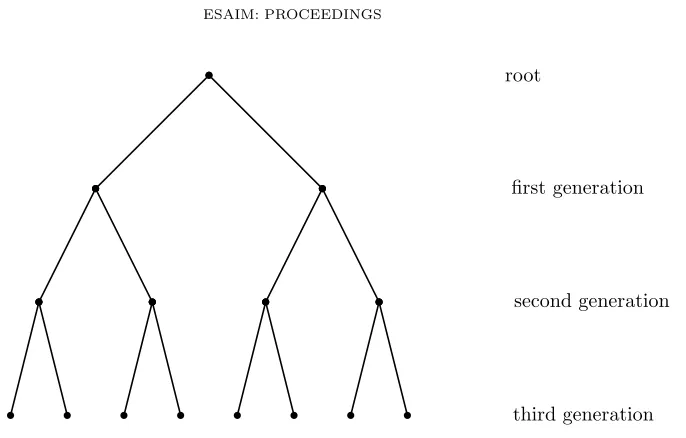
We are interested in processes involving (rooted) trees. The simplest rooted tree is the regular rooted
tree, where each vertex has a fixed number (saym, with m >1) of offspring. For example, here is a rooted
binary tree:
Let Zn denote the number of vertices (also called particles or individuals) in the n-th generation, then
Zn =mn,∀n≥0.
In probability theory, we often encounter trees where the number of offspring of a vertex is random. The
easiest case is when these random numbers are i.i.d., which leads to a Galton–Watson tree1.
A Galton–Watson tree starts with one initial ancestor (sometimes, it is possible to have several or even a
random number of initial ancestors, in which case it will be explicitly stated). It produces a certain number
of offspring according to a given probability distribution. The new particles form the first generation. Each
of the new particles produces offspring according to the same probability distribution, independently of each
root
first generation
second generation
third generation
Figure 1: First generations in a rooted binary tree
other and of everything else in the generation. And the system regenerates. We writepi for the probability
that a given particle hasi children, i≥0; thus P∞i=0pi = 1. [In the case of a regularm-ary tree, pm = 1
andpi= 0 fori6=m.]
To avoid trivial discussions, we assume throughout thatp0+p1<1.
As before, we writeZn for the number of particles in then-th generation. It is clear that ifZn= 0 for a
certainn, thenZj = 0 for allj≥n.
Figure 2: First generations in a Galton–Watson tree
In Figure 2, we haveZ0= 1,Z1= 2,Z2= 4,Z3= 7.
One of the first questions we ask is about the extinction probability
It turns out that the expected number of offspring plays an important role. Let
m:=E(Z1) = ∞
X
i=0
ipi∈(0,∞]. (1.2)
Theorem 1.1. Let qbe the extinction probability defined in (1.1).
(i)The extinction probability q is the smallest root of the equationf(s) =sfor s∈[0,1], where
f(s) := ∞
X
i=0
sipi, (00:= 1)
is the generating function of the reproduction law.
(ii)In particular, q= 1 ifm≤1, and q <1 ifm >1.
Proof. By definition, f(s) =E(sZ1). Conditioning onZn−1, Zn is the sum ofZn−1 i.i.d. random variables having the common distribution which is that ofZ1; thusE(sZn|Zn−1) =f(s)Zn−1, which impliesE(sZn) =
E(f(s)Zn−1). By induction,E(sZn) =fn(s) for anyn≥1, wherefn denotes then-th fold composition off.
In particular,P(Zn= 0) =fn(0).
The event{Zn= 0} being non-decreasing inn(i.e.,{Zn= 0} ⊂ {Zn+1= 0}), we have
q=P [
n
{Zn= 0}= lim
n→∞P(Zn= 0) = limn→∞fn(0).
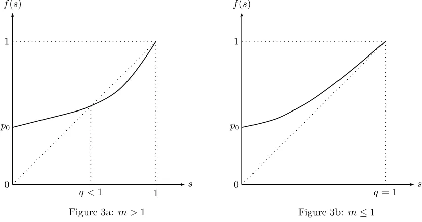
Let us look at the graph of the function f on [0,1]. The function is (strictly) increasing and strictly
convex, withf(0) =p0≥0 andf(1) = 1. In particular, it has at most two fixed points.
0
p0 1
1
q <1 s
f(s)
0
p0 1
q= 1 s
f(s)
Figure 3a: m >1 Figure 3b: m≤1
Ifm≤1, thenp0>0, and f(s)> sfor alls∈[0,1), which implies fn(0)→1. In other words,q= 1 is
Assume nowm∈(1,∞]. This time,fn(0) converges increasingly to the unique root off(s) =s,s∈[0,1).
In particular,q <1.
Theorem 1.1 tells us that in the subcritical case (i.e.,m <1) and in the critical case (m= 1), the Galton–
Watson process dies out with probability 1, whereas in the supercritical case (m >1), the Galton–Watson
process survives with (strictly) positive probability. In the rest of the text, we will be mainly interested in
the supercritical casem >1. But for the time being, let us introduce
Wn:= Zn
mn, n≥0,
which is well-defined as long asm < ∞. It is clear that Wn is a martingale (with respect to the natural
filtration of (Zn), for example). Since it is non-negative, we have
Wn →W, a.s.,
for some non-negative random variableW. [We recall that if (ξn) is a sub-martingale with supnE(ξn+)<∞,
thenξn converges almost surely to a finite random variable. Apply this to (−Wn).]
By Fatou’s lemma, E(W) ≤ lim infn→∞E(Wn) = 1. It is, however, possible that W = 0. So it is important to know whenW is non-degenerate.
We make the trivial remark thatW = 0 if the system dies out. In particular, by Theorem 1.1, we have
W = 0 a.s. ifm≤1. What happens ifm >1?
We start with two simple observations. The first says that in general,P(W = 0) equalsq or 1, whereas the second tells us thatW is non-degenerate if the reproduction law admits a finite second moment.
Proposition 1.2. Assumem <∞. ThenP(W = 0) equals eitherq or1.
Proof. There is nothing to prove ifm≤1. So let us assume 1< m <∞.
By definition,2Zn+1=PZ1i=1Z (i)
n , whereZn(i),i≥1, are copies ofZn, independent of each other andZ1.
Dividing on both sides by mn and letting n→ ∞, it follows that mW is distributed as PZ1
i=1W(i), where
W(i), i ≥ 1, are copies of W, independent of each other and Z1. In particular, P(W = 0) = E[P(W = 0)Z1] =f(P(W = 0)), i.e.,P(W = 0) is a root off(s) =sfors∈[0,1]. In words,P(W = 0) =qor 1.
Exercise 1.3. If E(Z12)<∞andm >1, thensupnE(Wn2)<∞.
Exercise 1.4. If E(Z12)<∞andm >1, thenE(W) = 1, andP(W = 0) =q.
It turns out that the second moment condition in Exercise 1.4 can be weakened to an XlogX-type
integrability condition. Let log+x:= log max{x,1}.
2Usual notation: P
Theorem 1.5. (Kesten and Stigum [35])Assume1< m <∞. Then
E(W) = 1 ⇔ P(W >0|non-extinction) = 1 ⇔ E(Z1log+Z1)<∞.
Remark. (i) The conclusion in the Kesten–Stigum theorem can also be stated as E(W) = 1 ⇔ P(W = 0) =q⇔P∞i=1piilogi <∞.
(ii) The conditionE(Z1log+Z1)<∞may look technical. We will see in the next paragraph why this is
a natural condition.
1.2. Size-biased Galton–Watson trees
In order to introduce size-biased Galton–Watson processes, we need to view the tree as a random element
in a probability space (Ω,F, P).
LetU :={∅} ∪S∞
k=1(N∗)k, whereN∗:={1,2,· · · }.
Ifu,v∈U, we denote byuv the concatenated element, withu∅=∅u=u.
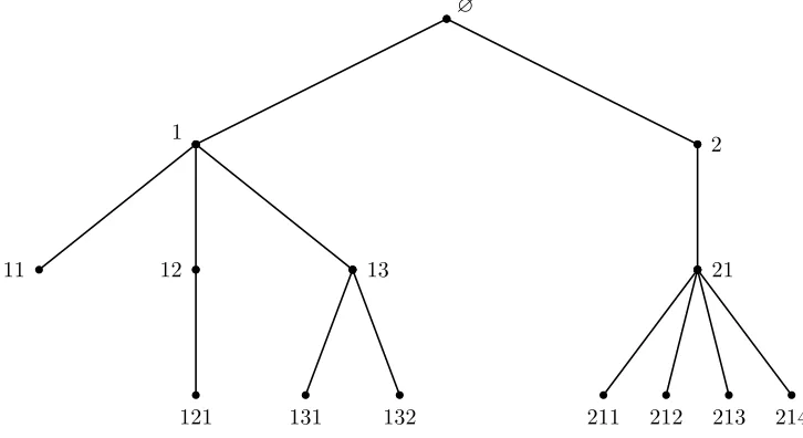
A treeω is a subset ofU satisfying: (i) ∅∈ω; (ii) if uj∈ω for somej∈N∗, then u∈ω; (iii) if u∈ω,
thenuj∈ω if and only if 1≤j≤Nu(ω) for some non-negative integerNu(ω).
In the language of trees, ifu∈U is an element of the treeω, uis a vertex of the tree, andNu(ω) the
number of children. Vertices ofωare labeled by their line of descent: ifu=i1· · ·in∈U, thenuis thein-th
child of thein−1-th child of . . . of thei1-th child of the initial ancestor∅.
∅
1 2
11 12 13 21
121 131 132 211 212 213 214
Figure 4: Vertices of a tree as elements ofU
Let Ω be the space of all trees. We now endow it with a sigma-algebra. For anyu∈U, let Ωu:={ω∈Ω :
because all the trees contain the root as a vertex, according to part (i) of the definition.] The promised
sigma-algebra associated with Ω is defined by
F :=σ{Ωu, u∈U}.
LetT: Ω→Ω be the identity application.
Let (pk, k≥0) be a probability. According to Neveu [44], there exists a probabilityPon Ω such that the law ofTunderPis the law of the Galton–Watson tree with reproduction distribution (pk).
LetFn:=σ{Ωu, u∈U, |u| ≤n}, where|u|is the length ofu(representing the generation of the vertex
uin the language of trees). Note thatF is the smallest sigma-field containing everyFn.
For any treeω∈Ω, letZn(ω) be the number of individuals in the n-th generation.3 It is easily checked
that for anyn,Zn is a random variable taking values inN:={0,1,2· · · }.
LetPb be the probability on (Ω,F) such that for anyn,
b
P|Fn =Wn•P|Fn,
i.e., P(b A) = RAWndP for any A ∈ Fn. Here, P|
Fn and P|b Fn are the restrictions of P and Pb on Fn,
respectively. SinceWn is a martingale, the existence ofPb is guaranteed by Kolmogorov’s extension theorem. For anyn,
b
P(Zn >0) =E[1{Zn>0}Wn] =E[Wn] = 1.
Therefore,P(b Zn>0, ∀n) = 1. In other words, there is almost surely non-extinction of the Galton–Watson tree T under the new probability P. The Galton–Watson treeb T under Pb is called a size-biased Galton–
Watson tree. Let us give a description of its paths.
LetN :=N∅. IfN ≥1, then there areN individuals in the first generation. We write T1, T2,· · ·, TN
for theN subtrees rooted at each of theN individual in the first generation.4
Exercise 1.6. Let k≥1. IfA1,A2,· · ·,Ak are elements of F, then
b
P(N =k, T1∈A1,· · ·,Tk∈Ak)
= kpk
m
1
k k
X
i=1
P(A1)· · ·P(Ai−1)P(b Ai)P(Ai+1)· · ·P(Ak). (1.3)
Equation (1.3) tells us the following fact about the size-biased Galton–Watson tree: The root has the
biased distribution, i.e., havingkchildren with probability kpk
m ; among the individuals in the first generation,
one of them is chosen randomly (according to the uniform distribution) such that the subtree rooted at this
3The rigorous definition isZ
n(ω) := #{u∈U : u∈ω, |u|=n}.
4The rigorous definition ofT
vertex is a size-biased Galton–Watson tree, whereas the subtrees rooted at all other vertices in the first
generation are independent copies of the usual Galton–Watson tree.
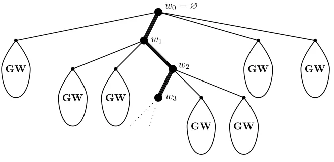
Iterating the procedure, we obtain a decomposition of the size-biased Galton–Watson tree with an (infinite)
spine and with i.i.d. copies of the usual Galton–Watson tree: The root∅=:w0has the biased distribution,
i.e., havingkchildren with probability kpk
m . Among the children of the root, one of them is chosen randomly
(according to the uniform distribution) as the element of the spine in the first generation (denoted by w1).
We attach subtrees rooted at all other children; these subtrees are independent copies of the usual Galton–
Watson tree. The vertexw1 has the biased distribution. Among the children of w1, we choose at random
one of them as the element of the spine in the second generation (denoted by w2). Independent copies of
the usual Galton–Watson tree are attached as subtrees rooted at all other children of w1, whereasw2 has
the biased distribution. And so on. See Figure 5.
b
b
b
b
GW GW GW
GW GW
GW GW
w0=∅
w1
w2
w3
Figure 5: A size-biased Galton–Watson tree
From technical point of view, it is more convenient to connect size-biased Galton–Watson trees with
Galton–Watson branching processes with immigration, described as follows.
A Galton–Watson branching processes with immigration starts with no individual (say), and is
charac-terized by a reproduction law and an immigration law. At generation n (forn ≥1), Yn new individuals
immigrate into the system, while all individuals regenerate independently and following the same
reproduc-tion law; we assume that (Yn, n≥1) is a collection of i.i.d. random variables following the same immigration
law, and independent of everything else in that generation.
Our description of the size-biased Galton–Watson tree can be reformulated in the following way: (Zn−
1, n≥0) underPb is a Galton–Watson branching process with immigration, whose immigration law is that ofNb−1, withP(Nb =k) := kpk
1.3. Proof of the Kesten–Stigum theorem
We prove the Kesten–Stigum theorem, by means of size-biased Galton–Watson trees. Let us start with a
few elementary results.
Exercise 1.7. Let X,X1,X2,· · · be i.i.d. non-negative random variables. (i)If E(X)<∞, then Xn
n →0 a.s.
(ii)If E(X) =∞, thenlim supn→∞Xnn =∞a.s.
For the next elementary results, let (Fn) be a filtration, and letPandPb be probabilities5on (Ω,F∞).
Assume that for any n, P|b Fn is absolutely continuous with respect to P|Fn. Let ξn :=
dPb|Fn
dP|Fn
, and let
ξ:= lim supn→∞ξn.
Exercise 1.8. Prove that(ξn)is aP-martingale. Prove thatξn →ξP-a.s., and that ξ <∞P-a.s.
Exercise 1.9. Prove that
b
P(A) =E(ξ1A) +P(b A∩ {ξ=∞}), ∀A∈F∞. (1.4)
Hint: You can first prove the identity assumingPb ≪Pand using L´evy’s martingale convergence theorem6. Exercise 1.10. Prove that
b
P≪P ⇔ ξ <∞, P-a.s.b ⇔ E(ξ) = 1, (1.5)
b
P⊥P ⇔ ξ=∞, P-a.s.b ⇔ E(ξ) = 0. (1.6)
The Kesten–Stigum theorem will be a consequence of Seneta [51]’s theorem for branching processes with
immigration.
Exercise 1.11. (Seneta’s theorem)Let Zn denote the number of individuals in then-th generation of a branching process with immigration (Yn). Assume that 1< m <∞, wherem denotes the expectation of the
reproduction law.
(i)If E(log+Y1)<∞, thenlim
n→∞mZnn exists and is finite a.s.
(ii)If E(log+Y1) =∞, thenlim sup
n→∞mZnn =∞, a.s.
Proof of the Kesten–Stigum theorem. Assume 1< m <∞.
IfP∞i=1piilogi <∞, then E(log+Nb)<∞. By Seneta’s theorem, lim
n→∞Wn exists P-a.s. and is finiteb
b
P-a.s. By (1.5),E(W) = 1; in particular,P(W = 0)<1 and thus P(W = 0) =q(Proposition 1.2). 5We denote byF
∞, the smallest sigma-algebra containing allFn.
6That is, ifηisP-integrable, thenE(η|F
IfP∞i=1piilogi=∞, thenE(log+Nb) =∞. By Seneta’s theorem, lim
n→∞WnexistsP-a.s. and is infiniteb
b
P-a.s. By (1.6),E(W) = 0, and thusP(W = 0) = 1.
1.4. The Seneta–Heyde norming
In the supercritical case, the Kesten–Stigum theorem (Theorem 1.5) tells us that under the condition
E(Z1log+Z1)<∞, mZnn converges almost surely to a limit (i.e., W), which vanishes precisely on the set of
extinction. It turns out that even without the conditionE(Z1log+Z1)<∞, the conclusion still holds true if we are allowed to modify the normalizing function.
Theorem 1.12. (Seneta [50], Heyde [31])Assume 1 < m < ∞. Then there exists a sequence (cn) of positive constants such that cn+1
cn →m and that
Zn
cn has a (finite) almost sure limit vanishing precisely on
the set of extinction.
Proof. We note thatf−1is well-defined on [p 0,1].
Lets0∈(q, 1) and define by inductionsn:=f−1(sn−1),n≥0. Clearly,sn↑1.
Conditioning on Fn−1, Zn is the sum ofZn−1 i.i.d. random variables having the common distribution
which is that ofZ1; thusE(sZn
n |Fn−1) =f(sn)Zn−1, which implies thatsZnn is a martingale. Since it is also
bounded, it converges almost surely and inL1to a limit7, sayY, withE(Y) =E(sZ0
0 ) =s0.
Letcn := 1
log(1/sn),n≥0. By definition,s
Zn
n = e−Zn/cn, so that limn→∞ Zcnn exists a.s., and lies in [0,∞]. By l’Hˆopital’s rule,
lim
s→1
logf(s) logs = lims→1
f′(s)s
f(s) =m. This yields cn+1
cn →m.
Consider the setA :={limn→∞Zcnn = 0}. Let as beforeT1,· · ·, TZ1 denote the subtrees rooted at each
of the individuals in the first generation. Then8
P(A) =P(T∈A) =E{P(T∈A|Z1)} ≤E{P(T1∈A,· · · ,TZ1 ∈A|Z1)},
the inequality being a consequence of the fact that cn+1
cn →m. SinceT1,· · ·,TZ1 are i.i.d. givenZ1, we have
P(T1∈A,· · · ,TZ1 ∈A|Z1) = [P(A)]Z1; therefore,P(A)≤E{[P(A)]Z1}=f(P(A)).
On the other hand, P(A)≥q. ThusP(A)∈ {q,1}, andP(A|non-extinction) ∈ {0,1}. SinceE(Y) =
s0 < 1, this yields P(A|non-extinction) = 0; in other words, {limn→∞Zcnn = 0} = {extinction} almost surely.
Similarly, we can poseB :={limn→∞Zcnn <∞} and check thatP(B)≤f(P(B)). Since P(B)≥q, we haveP(B|non-extinction)∈ {0,1}. Now,E(Y) =s0> q, we obtainP(B|non-extinction) = 1.
7We use the fact that if (ξ
n) is a martingale withE(supn|ξn|)<∞, then it converges almost surely and inL1.
Remark. Of course9, in the Seneta–Heyde theorem, we havecn≈mn if and only ifE(Z
1log+Z1)<∞.
1.5. Notes
Subsection 1.1 concerns elementary properties of Galton–Watson processes. For a general account, we
refer to standard books such as Asmussen and Hering [3], Athreya and Ney [4], Harris [30].
The formulation of branching processes described at the beginning of Subsection 1.2 is due to Neveu [44];
the idea of viewing Galton–Watson branching processes as tree-valued random variables can be found in
Harris [30].
The idea of size-biased branching processes, which goes back at least to Kahane and Peyri`ere [33], has
been used by several authors in various contexts. Its presentation in Subsection 1.2, as well as its use to prove
the Kesten–Stigum theorem, comes from Lyons, Pemantle and Peres [41]. Size-biased branching processes
can actually be used to prove the corresponding results of the Kesten–Stigum theorem in the critical and
subcritical cases. See [41] for more details.
The short proof of Seneta’s theorem (Exercise 1.11) is borrowed from Asmussen and Hering [3], pp. 50–51.
The Seneta–Heyde theorem (Theorem 1.12) was first proved by Seneta for convergence in distribution,
and then by Heyde for almost sure convergence. The short proof is from Lyons and Peres [42]. For another
simple proof, see Grey [25].
2. Branching random walks and the law of large numbers
The Galton–Watson branching process simply counts the number of particles in each generation. In this
section, we make an extension in the spatial sense by associating each individual of the Galton–Watson
process with a random variable. This results to a branching random walk.
We first study a simple example of branching random walk; in particular, the idea of using the Cram´er–
Chernoff large deviation theorem appears in a natural way. We then put this idea into a general setting,
and prove a law of large numbers for the branching random walk. Our basic technique relies, once again,
on (a spatial version of) size-biased trees. In particular, this technique also gives a spatial version of the
Kesten–Stigum theorem, namely, the Biggins martingale convergence theorem.
2.1. Warm-up
We study a simple example of branching random walk in this paragraph. LetTbe a binary tree rooted
at∅. Let (ξx, x∈T) be a collection10of i.i.d. random variables indexed by all the vertices ofT. To simplify
the situation, we assume that the common distribution ofξxis the uniform distribution on [0,1].
For any vertexx∈T, let [[∅, x]] denote the shortest path connecting∅tox. Ifxis in then-th generation,
then [[∅, x]] is composed ofn+ 1 vertices, each one is the parent of the next vertex whereas the last vertex
9Bya
n≈bn, we mean 0<lim infn→∞an
bn ≤lim supn→∞
an
bn <∞.
is simplyx. Let ]]∅, x]] := [[∅, x]]\{∅}. We defineV(∅) := 0 and
V(x) := X
y∈]]∅, x]]
ξy, x∈T\{∅}.
Then (V(x), x ∈T) is an example of branching random walk which we study in its generality in the next
subsection. For the moment, we continue with our example.
For anyxin then-th generation,V(x) is by definition sum ofni.i.d. uniform-[0,1] random variables, so
by the usual law of large numbers,V(x) would be approximatively n
2 whennis large. We are interested in
the asymptotic behaviour, whenn→ ∞, of11
1
n|xinf|=nV(x).
If, with probability one, γ := limn→∞1ninf|x|=nV(x) exists and is a constant, then γ ≤ 12 according to
the above discussion. A little more thought will convince us that the inequality would be strict: γ < 12. Here
is why.
Let s ∈ (0, 1
2). For any |x| = n, the probability P{V(x) ≤ sn} goes to 0 when n→ ∞ (weak law of large numbers); this probability is exponentially small (the Cram´er–Chernoff theorem12): P{V(x)≤sn} ≈ exp(−I(s)n), for some constantI(s)>0 depending onswhich is explicitly known. LetN(s, n) be the number
of x in the n-th generation such that V(x) ≤ sn. Then E(N(s, n)) is approximatively 2nexp(−I(s)n).
In particular, if I(s) < log 2, then E(N(s, n)) → ∞, and one would expect that N(s, n) would be at least one when n is sufficiently large. If indeed N(s, n) ≥1, then inf|x|=nV(x) ≤ sn, which would yield
γ≤s < 12. On the other hand, ifI(s)>log 2, then by Chebyshev’s inequalityP{N(s, n)≥1} ≤E(N(s, n)),
P
nP{N(s, n)≥1}<∞, so a Borel–Cantelli argument tells thatγ≥s.
If the heuristics were true, then one would getγ= inf{s <12 : I(s)<log 2}= sup{s < 12: I(s)>log 2}
(admitting that the last identity holds).
In the next subsections, we will develop the heuristics into a rigorous argument. We will prove the Biggins
martingale convergence theorem (which is a spatial version of the Kesten–Stigum theorem) by means of
size-biased branching random walks; the martingale convergence theorem allows us to avoid discussing the
technical point about whetherN(s, n)≥1 whenE(N(s, n)) is very large.
2.2. Law of large numbers
The (discrete-time one-dimensional) branching random walk is a natural extension of the Galton–Watson
tree in the spatial sense; its distribution is governed by a point process which we denote by Θ.
11Throughout,|x|denote the generation of the vertexx.
An initial ancestor is born at the origin of the real line. Its children, who form the first generation, are
positioned according to the point process Θ. Each of the individuals in the first generation produces children
who are thus in the second generation and are positioned (with respect to their born places) according to
the same point process Θ. And so on. We assume that each individual reproduces independently of each
other and of everything else. The resulting system is called a branching random walk.
It is clear that if we only count the number of individuals in each generation, we get a Galton–Watson
process, with #Θ being its reproduction distribution.
The example in Subsection 2.1 corresponds to the special case that the point process Θ consists of two
independent uniform-[0,1] random variables.
Let (V(x),|x|=n) denote the positions of the individuals in then-th generation. We are interested in
the asymptotic behaviour of inf|x|=nV(x).
Let us introduce the (log-)Laplace transform of the point process
ψ(t) := logE X |x|=1
e−tV(x)∈(−∞,∞], t≥0. (2.7)
Throughout this section, we assume:
•ψ(t)<∞for somet >0;
•ψ(0)>0.
The assumptionψ(0)>0 is equivalent toE(#Θ)>1, i.e., the associated Galton–Watson tree is supercritical. The main result of this section is as follows.
Theorem 2.1. If ψ(0)>0 andψ(t)<∞ for somet >0, then almost surely on the set of non-extinction,
lim
n→∞ 1
n|xinf|=nV(x) =γ,
where
γ:= inf{a∈R: J(a)>0}, J(a) := inf
t≥0[ta+ψ(t)], a∈
R. (2.8)
If instead we want to know about sup|x|=nV(x), we only need to replace the point process Θ by−Θ.
Theorem 2.1 is proved in Subsection 2.3 for the lower bound, and in Subsection 2.5 for the upper bound.
We close this paragraph with a few elementary properties of the functionsJ(·) andψ(·). We assume that
ψ(t)<∞for somet >0.
Clearly,J is concave, being the infimum of concave (linear) function; in particular, it is continuous on the
interior of{a∈R: J(a)>−∞}. Also, it is obvious thatJ is non-decreasing.
We recall that a function f is said to be lower semi-continuous at point t if for any sequencetn → t,
is well-known and easily checked by definition that f is lower semi-continuous if and only if for anya∈R,
{t:f(t)≤a} is closed.
Exercise 2.2. Prove thatψ is convex and lower semi-continuous on [0, ∞).
Exercise 2.3. Assume that ψ(t)<∞for somet >0. Then for any t≥0,
ψ(t) = sup
a∈R
[J(a)−at].
Hint: A property of the Legendre transformationf∗(x) := sup
a∈R(ax−f(a)): a functionf :R→(−∞,∞]
is convex and lower semi-continuous if and only if13(f∗)∗ =f.
Exercise 2.4. Assume that ψ(t)<∞for somet >0. Then
γ= sup{a∈R: J(a)<0}
Furthermore,γ is the unique solution ofJ(γ) = 0.
2.3. Proof of the law of large numbers: lower bound
Fix ana∈Rsuch that J(a)<0. Let
Ln =Ln(a) := X |x|=n
1{V(x)≤na}.
By Chebyshev’s inequality,P(Ln >0) =P(Ln≥1)≤E(Ln). Let t≥0. Since1{V(x)≤na}≤enat−tV(x), we have
P(Ln >0)≤enatE X |x|=n
e−tV(x).
To compute the expectation expression on the right-hand side, let Fk (for anyk) be the sigma-algebra
generated by the firstk generations of the branching random walk; then
E(X |x|=n
e−tV(x)|Fn−1) = X
|y|=n−1
e−tV(y)eψ(t).
Taking expectation on both sides gives E(P|x|=ne−tV(x)) = eψ(t)E(P
|x|=n−1e−tV(x)), which is enψ(t) by
induction. As a consequence, P(Ln >0)≤ enat+nψ(t), for anyt ≥0. Taking infimum over all t≥0, this leads to:
P(Ln>0)≤expninf
t≥0(at+ψ(t))
= enJ(a).
By assumption,J(a)<0, so thatPnP(Ln>0)<∞. By the Borel–Cantelli lemma, with probability one, for all sufficiently largen, we haveLn= 0, i.e., inf|x|=nV(x)> na. The lower bound in Theorem 2.1 follows.
2.4. Size-biased branching random walk and martingale convergence
Letβ∈Rbe such thatψ(β) := logE{P
|x|=1e−βV(x)} ∈R. Let
Wn(β) := 1 enψ(β)
X
|x|=n
e−βV(x)= X |x|=n
e−βV(x)−nψ(β), n≥1.
[Whenβ= 0,Wn(0) is the martingale we studied in Section 1.] Using the branching structure, we
immedi-ately see that (Wn(β), n≥1) is a martingale with respect to (Fn), whereFn is the sigma-field induced by
the firstngenerations of the branching random walk. Therefore,Wn(β)→W(β) a.s., for some non-negative
random variableW(β). Fatou’s lemma says thatE[W(β)]≤1.
Here is Biggins’s martingale convergence theorem, which is the analogue of the Kesten–Stigum theorem
for the branching random walk.
Theorem 2.5. (Biggins [8]) If ψ(β) < ∞ and ψ′(β) := −e−ψ(β)E{P
|x|=1V(x)e−βV(x)} exists and is
finite, then
E[W(β)] = 1 ⇔ P{W(β)>0|non-extinction}= 1
⇔ E[W1(β) log+W1(β)]<∞ andβψ′(β)< ψ(β).
A similar remark as in the Kesten–Stigum theorem applies here: the condition
P{W(β)>0|non-extinction}= 1,
which meansP[W(β) = 0] = q, is easily seen to be equivalent toP[W(β) = 0]<1 via a similar argument as in Proposition 1.2.
The proof of the theorem relies the notion of size-biased branching random walks, which is an extension in
the spatial sense of size-biased Galton–Watson processes. We only describe the main idea; for more details,
we refer to Lyons [40].
Some basic notation is in order (for more details, see Neveu [44]). Let U := {∅} ∪S∞
k=1(N∗)k as in
Subsection 1.2. LetU :={(u, V(u)) : u∈U, V :U →R}. Let Ω be Neveu’s space ofmarkedtrees, which
consists of all the subsetsωofU such that the first component ofω is a tree. [Attention: Ω is different from
the Ω in Subsection 1.2.] LetT: Ω→Ω be the identity application. According to Neveu [44], there exists
a probabilityPon Ω such that the law ofTunderPis the law of the branching random walk described in
the previous section.
According to Kolmogorov’s extension theorem, there exists a unique probabilityPb =P(b β) on Ω such that for anyn≥1,
b
The law ofTunderPb is called the law of a size-biased branching random walk.
Here is a simple description of the size-biased branching random walk (i.e., the distribution of the branching
random walk underP). The offspring of the rootb ∅=:w0is generated according to the biased distribution14
b
Θ =Θ(b β). Pick one of these offspringw1at random; the probability that a given vertexxis picked up asw1
is proportional to e−βV(x). The children other thanw
1give rise to independent ordinary branching random
walks, whereas the offspring ofw1is generated according to the biased distributionΘ (and independently ofb
others). Again, pick one of the children ofw1 at random with probability which is inversely exponentially
proportional to (β times) the displacement, call itw2, with the others giving rise to independent ordinary
branching random walks whilew2produce offspring according to the biased distributionΘ, and so on.b
Proof of Theorem 2.5. If β = 0 or if the point process Θ is deterministic, then Theorem 2.5 is reduced to
the Kesten–Stigum theorem (Theorem 1.5) proved in the previous section. So let us assume thatβ 6= 0 and
that Θ is not deterministic.
(i) Assume the condition on the right-hand side fails. We claim that in this case, lim supn→∞Wn(β) =∞
b
P-a.s.; thus by (1.6),E[W(β)] = 0; a fortiori,P{W(β)>0|non-extinction}= 0. To see why lim supn→∞Wn(β) =∞P-a.s., we distinguish two possibilities.b First possibility: βψ′(β)≥ψ(β). Then
lim sup
n→∞ [−
βV(wn)−nψ(β)] =∞, P-a.s.b
[This is obvious ifβψ′(β)> ψ(β), because by the law of large numbers,
V(wn)
n →EPb[V(w1)] =E[
X
|x|=1
V(x)e−βV(x)−ψ(β)] =−ψ′(β), P-a.s.b
Ifβψ′(β) =ψ(β), then the law of large numbers says V(wn)
n → −
ψ(β)
β ,P-a.s., and we still haveb
15
lim inf
n→∞[βV(wn) +nψ(β)] =−∞, P-a.s.]b SinceWn(β)≥e−βV(wn)−nψ(β), we immediately get lim sup
n→∞Wn(β) =∞P-a.s., as desired.b Second possibility: E[W1(β) log+W1(β)] =∞. In this case, we argue that
Wn+1(β) = X |x|=n
e−βV(x)−(n+1)ψ(β) X |y|=n+1, y>x
e−β[V(y)−V(x)]
≥ e−βV(wn)−(n+1)ψ(β) X
|y|=n+1, y>wn
e−β[V(y)−V(wn)]=:In×IIn.
14That is, a point process whose distribution (underP) is the distribution of Θ underPb.
15It is an easy consequence of the central limit theorem that ifX1,X2,· · · are i.i.d. random variables withE(X1) = 0 and
E(X2
1)<∞, then lim supn→∞ Pn
SinceIIn are i.i.d. (underP) withb EPb(log+II0) =E[W1(β) log+
W1(β)] =∞, it follows from Exercise 1.7 (ii)
that
lim sup
n→∞ 1
nlog
+IIn=∞, P-a.s.b On the other hand, V(wn)
n → −ψ
′(β),P-a.s. (law of large numbers), this yields lim supb
n→∞In×IIn =∞,
b
P-a.s., which, again, leads to lim supn→∞Wn(β) =∞P-a.s.b
(ii) We now assume that the condition on the right-hand side of the Biggins martingale convergence
theorem is satisfied, i.e., βψ′(β) < ψ(β) and E[W1(β) log+W1(β)] < ∞. Let G be the sigma-algebra
generated bywn andV(wn) as well as offspring ofwn, for alln≥0. Then
EPb[Wn(β)|G] =
n−1
X
k=0
e−βV(wk)−(n+1)ψ(β) X
|x|=k+1:x>wk, x6=wk+1
e−β[V(x)−V(wk)]e[n−(k+1)]ψ(β)
+e−βV(wn)−(n+1)ψ(β)
=
n−1
X
k=0
e−βV(wk)−(k+1)ψ(β) X
|x|=k+1:x>wk
e−β[V(x)−V(wk)]−
n−1
X
i=1
e−βV(wi)−iψ(β)
=
n−1
X
k=0
Ik×IIk−eψ(β)
nX−1
i=1
Ii.
SinceIIn are i.i.d. (underP) withb EPb(log+II0) =E[W1(β) log+W1(β)]<∞, it follows from Exercise 1.7 (i) that
lim
n→∞ 1
nlog
+IIn= 0, P-a.s.b
On the other hand,In decays exponentially fast (becauseβψ′(β)< ψ(β)). It follows that Pn−1
k=0Ik×IIk− eψ(β)Pn−1
i=1 Ik convergesP-a.s. By (the conditional version of) Fatou’s lemma,b EPb{lim infn→∞Wn(β)|G}<
∞,P-a.s.b
Recall thatP|Fn =
1
Wn(β)•P|b Fn. We claim that
1
Wn(β) is aP-supermartingaleb
16: indeed, for anyn≥j
and A ∈ Fj, we have Eb
P[ 1
Wn(β)1A] = P{Wn(β) > 0, A} ≤ P{Wj(β) > 0, A} = EPb[
1
Wj(β)1A], thus
EPb[ 1
Wn(β)|
Fj]≤ 1
Wj(β) as claimed. Since
1
Wn(β) is a positiveP-supermartingale, it convergesb P-a.s., to ab
limit which, according to what we have proved in the last paragraph, isP-almost surely (strictly) positive.b We can write as follow: lim supn→∞Wn(β)<∞,P-a.s. According to (1.5), this yieldsb E[W(β)] = 1, which obviously impliesP[W(β) = 0]<1, and which is equivalent toP{W(β)>0|non-extinction}= 1 as pointed out in the remark after Theorem 2.5. This completes the proof of Theorem 2.5.
We end this paragraph with the following re-statement of the size-biased branching random walk: for
any n ≥ 1, P|b Fn := Wn(β)•P|Fn, P(b wn = x|Fn) =
e−βV(x) P
|y|=ne−βV(y) =
e−βV(x)−nψ(β)
Wn(β) for any |x| = n;
under P, we have an (infinite) spine and i.i.d. copies of the usual branching random walk. Along theb 16In general, 1
spine, V(wi)−V(wi−1), i ≥ 1, are i.i.d. under P, and the distribution ofb V(w1) under Pb is given by EPb[F(V(w1))] =E{P|x|=1F(V(x))e−βV(x)−ψ(β)}, for any measurable functionF:R→R+.
b
b
b
b
BRW BRW BRW
BRW BRW
BRW BRW
w0=∅
w1
w2
w3
Figure 6: A size-biased branching random walk
Here is a consequence of the decomposition of the size-biased branching random walk, which will be of
frequent use.
Corollary 2.6. Assumeψ(β)<∞. Then for any n≥1 and any measurable function g:R→R+,
En X |x|=n
e−βV(x)−nψ(β)g(V(x))o=E[g(Sn)], (2.9)
whereSn :=Pni=1Xi, and(Xi) is a sequence of i.i.d. random variables such that
E[F(X1)] =E{X
|x|=1
F(V(x))e−βV(x)−ψ(β)},
for any measurable function F:R→R+.
Proof of Corollary 2.6. Let LHS(2.9) denote the expression on the left hand-side of (2.9). By definition,
LHS(2.9) = EPb{
P
|x|=ne
−βV(x)−nψ(β)
Wn(β) g(V(x))}. Recall that P(b wn = x|
Fn) = e−βV(x)−nψ(β)
Wn(β) , this yields
LHS(2.9)=EPb{
P
|x|=n1{wn=x}g(V(x))}, which isEPb[g(V(wn))]. It remains to recall thatV(wi)−V(wi−1),
i≥1, are i.i.d. underPb having the distribution ofX1.
2.5. Proof of the law of large numbers: upper bound
We prove the upper bound in the law of large numbers under the additional assumptions thatψ(t)<∞,
Exercise 2.7. Assume that ψ(t)<∞,∀t≥0, and that ψ(0)>0. Leta∈Rbe such that0< J(a)< ψ(0). Then there existsβ >0 such that ψ′(β) =−a.
Let a∈ R be such that 0 < J(a) < ψ(0). According to Exercise 2.7, ψ′(β) = −afor some β >0. In
particular, 0< J(a) =aβ+ψ(β) =−βψ′(β) +ψ(β).
LetWn(β) :=P|x|=ne−βV(x)−nψ(β) as before. Letε >0 and let
∆n :=
X
|x|=n:|V(x)−na|>εn
e−βV(x)−nψ(β).
By Corollary 2.6 and in its notation, E(∆n) = P(|Sn−na|> εn). Recall thatSn =Pni=1Xi, with (Xi)
i.i.d. such that E[F(X1)] = E{P|x|=1F(V(x))e−βV(x)−ψ(β)}, for any measurable function F : R → R+. In particular,E(X1) =a. By the Cram´er–Chernoff large deviation theorem, PnP(|Sn−na| > εn)<∞.
Therefore,Pn∆n<∞a.s. In particular, ∆n →0, a.s.
By definition,
Wn(β) = X |x|=n:|V(x)−na|≤εn
e−βV(x)−nψ(β)+ ∆n
≤ e−βn(a−ε)−nψ(β)#{|x|=n: V(x)≤(a+ε)n}+ ∆n.
We know ∆n→0 a.s., so that
lim inf
n→∞ e
−βn(a−ε)−nψ(β)#{|x|=n: V(x)≤(a+ε)n} ≥W(β), a.s.
Since βψ′(β) < ψ(β) and E[W1(β) log+W1(β)] < ∞, it follows from the Biggins martingale convergence theorem (Theorem 2.5) thatWn(β)→W(β)>0 almost surely on non-extinction. As a consequence, on the
set of non-extinction,
lim sup
n→∞ 1
n|xinf|=nV(x)≤a+ε, a.s.
This completes the proof of the upper bound in Theorem 2.1.
2.6. Notes
The law of large numbers (Theorem 2.1) was first proved by Hammersley [26] for the Bellman–Harris
process, by Kingman [36] for the (strictly) positive branching random walk, and by Biggins [7] for the
branching random walk.
The proof of the upper bound in the law of large numbers, presented in Subsection 2.5 based on martingale
convergence, is not the original proof given by Biggins [7]. Biggins’ proof relies on constructing an auxiliary
branching process, as suggested by Kingman [36].
The short proof of the Biggins martingale convergence theorem in Subsection 2.4, via size-biased branching
3. Branching random walks and the central limit theorem
We continue our study of the branching random walk. In Subsection 3.1, we state the main result, a central
limit theorem for the minimal position in the branching random walk. We do not directly study the minimal
position, but rather investigate some martingales involvingallthe living particles in the same generation, but
to which only the minimal positions make significant contributions. The study of these martingales relies,
again, on the idea of size-biased branching random walks, and is also connected to problems for directed
polymers on a tree. Unfortunately, our central limit theorem does not apply to all branching random walks;
a particular pathological case is analyzed in Subsection 3.9. At the end of the section, we mention a few
related models of branching random walks.
3.1. Central limit theorem
Let (V(x), |x|=n) denote the positions of the branching random walk. The law of large numbers proved
in the previous section states that conditional on non-extinction,
lim
n→∞ 1
n|xinf|=nV(x) =γ, a.s.,
whereγ is the constant in (2.8). It is natural to ask about the rate of convergence in this theorem.
Let us look at the special case of i.i.d. random variables assigned to the edges of a rooted regular tree. It
turns out that inf|x|=nV(x) has few fluctuations with respect to, say, its medianmV(n). In fact, the law
of inf|x|=nV(x)−mV(n) is tight! This was first proved by Bachmann [5] for the branching random walk
under the technical condition that the common distribution of the i.i.d. random variables assigned on the
edges of the regular tree admits a density function which is log-concave (a most important example being
the Gaussian law). This technical condition was recently removed by Bramson and Zeitouni [15]. See also
Subsection 5 of the survey paper by Aldous and Bandyopadhyay [2] for other discussions. Finally, let us
mention the recent paper of Lifshits [38], where an example of branching random walk is constructed such
that the law of inf|x|=nV(x)−mV(n) is tight but does not converge weakly.
Throughout the section, we assume that for someδ >0,δ+>0 andδ−>0,
En X
|x|=1
11+δo < ∞, (3.10)
En X |x|=1
e−(1+δ+)V(x)o+En X |x|=1
eδ−V(x)o < ∞, (3.11)
We recall the log-Laplace transform
ψ(t) := logEn X |x|=1
By (3.11),ψ(t)<∞fort∈[−δ−,1 +δ+]. Following Biggins and Kyprianou [11], we assume17
ψ(0)>0, ψ(1) =ψ′(1) = 0. (3.12)
For comments on this assumption, see Remark (ii) below after Theorem 3.1.
Under (3.12), the value of the constantγ defined in (2.8) is γ = 0, so that Theorem 2.1 reads: almost
surely on the set of non-extinction,
lim
n→∞ 1
n|xinf|=nV(x) = 0. (3.13)
On the other hand, under (3.12), Theorem 2.5 tells us thatP|x|=ne−V(x)→0 a.s., which yields that, almost
surely,
inf
|x|=nV(x)→+∞.
In other words, on the set of non-extinction, the system is transient to the right.
A refinement of (3.13) is obtained by McDiarmid [43]. Under the additional assumptionE{(P|x|=11)2}<
∞, it is proved in [43] that for some constantc1<∞and conditionally on the system’s non-extinction,
lim sup
n→∞ 1
logn |xinf|=nV(x)≤c1, a.s.
We now state a central limit theorem.
Theorem 3.1. Assume(3.10),(3.11)and(3.12). On the set of non-extinction, we have
lim sup
n→∞ 1
logn|xinf|=nV(x) =
3
2, a.s. (3.14)
lim inf
n→∞ 1
logn|xinf|=nV(x) =
1
2, a.s. (3.15)
lim
n→∞ 1
logn|xinf|=nV(x) =
3
2, in probability. (3.16)
Remark. (i) The most interesting part of Theorem 3.1 is possibly (3.14)–(3.15). It reveals the presence of fluctuations of inf|x|=nV(x) on the logarithmic level, which is in contrast with a known result of Bramson [14]
stating that for a class of branching random walks, 1
log logninf|x|=nV(x) converges almost surely to a finite
and positive constant.
(ii) Some brief comments on (3.12) are in order. In general (i.e., without assumingψ(1) =ψ′(1) = 0), if
t∗ψ′(t∗) =ψ(t∗) (3.17)
for somet∗∈(0,∞), then the branching random walk associated with the point processVb(x) :=t∗V(x) +
ψ(t∗)|x|satisfies (3.12). That is, as long as (3.17) has a solution (which is the case for example if ψ(1) = 0
andψ′(1)>0), the study will boil down to the case (3.12).
It is, however, possible that (3.17) has no solution. In such a situation, Theorem 3.1 does not apply. For
example, we have already mentioned a class of branching random walks exhibited in Bramson [14], for which
inf|x|=nV(x) has an exotic log lognbehaviour. See Subsection 3.9 for more details.
(iii) Under (3.12) and suitable integrability assumptions, Addario-Berry and Reed [1] obtain a very precise
asymptotic estimate ofE[inf|x|=nV(x)], as well as an exponential upper bound for the deviation probability
for inf|x|=nV(x)−E[inf|x|=nV(x)], which, in particular, implies (3.16).
(iv) In the case of (continuous-time) branching Brownian motion, a refined version of the analogue of
(3.16) was proved by Bramson [13], by means of some powerful explicit analysis.
3.2. Directed polymers on a tree
The following model is borrowed from the well-known paper of Derrida and Spohn [22]: LetTbe a rooted
Cayley tree; we study all self-avoiding walks (= directed polymers) ofnsteps onTstarting from the root. To
each edge of the tree, is attached a random variable (= potential). We assume that these random variables
are independent and identically distributed. For each walkω, its energyE(ω) is the sum of the potentials
of the edges visited by the walk. So the partition function is
Zn(β) :=X
ω
e−βE(ω),
where the sum is over all self-avoiding walks ofnsteps onT, andβ >0 is the inverse temperature.18
More generally, we take T to be a Galton–Watson tree, and observe that the energy E(ω) corresponds
to (the partial sum of) the branching random walk described in the previous paragraphs. The associated
partition function becomes
Zn,β:= X |x|=n
e−βV(x), β >0. (3.18)
If 0< β <1, the study ofZn,βboils down to the caseψ′(1)<0 which is covered by the Biggins martingale
convergence theorem (Theorem 2.5). In particular, on the set of non-extinction, Zn,β
E{Zn,β} converges almost
surely to a (strictly) positive random variable.
We now study the caseβ ≥1. Ifβ= 1, we write simply Zn instead ofZn,1.
Theorem 3.2. Assume(3.10),(3.11)and(3.12). On the set of non-extinction, we have
Zn=n−1/2+o(1), a.s. (3.19)
18There is hopefully no confusion possible between Z
n here and the number of individuals in a Galton–Watson process
Theorem 3.3. Assume(3.10),(3.11)and(3.12), and let β >1. On the set of non-extinction, we have
lim sup
n→∞
logZn,β
logn = − β
2, a.s. (3.20)
lim inf
n→∞
logZn,β
logn = −
3β
2 , a.s. (3.21)
Zn,β = n−3β/2+o(1), in probability. (3.22)
Again, the most interesting part in Theorem 3.3 is probably (3.20)–(3.21), which describes a new
fluctu-ation phenomenon. Also, there is no phase transition any more forZn,β at β= 1 from the point of view of
upper almost sure limits.
An important step in the proof of Theorems 3.2 and 3.3 is to estimate all small moments ofZn andZn,β,
respectively. This is done in the next theorems.
Theorem 3.4. Assume(3.10),(3.11)and(3.12). For anya∈[0,1), we have
0<lim inf
n→∞ E
n
(n1/2Zn)ao≤lim sup
n→∞ E
n
(n1/2Zn)ao<∞.
Theorem 3.5. Assume(3.10),(3.11)and(3.12), and let β >1. For any 0< r <β1, we have
EZn,βr =n−3rβ/2+o(1), n→ ∞. (3.23)
We prove the theorems of this section under the additional assumption that for some constant C,
sup|x|=1|V(x)|+ #{x: |x| = 1} ≤C a.s. This assumption is not necessary, but allows us to avoid some
technical discussions.
3.3. Small moments of partition function: upper bound in Theorem 3.5
This subsection is devoted to (a sketch of) the proof of the upper bound in Theorem 3.5; the upper bound
in Theorem 3.4 can be proved in a similar spirit, but needs more care.
We assume (3.10), (3.11) and (3.12), and fixβ >1.
LetPb be such thatP|bFn =Zn•P|Fn,∀n. For anyY ≥0 which isFn-measurable, we haveE{Zn,βY}=
EPb{P|x|=ne−βVZn(x)Y}=EPb{P|x|=n1{wn=x}e
−(β−1)V(x)Y}, and thus
E{Zn,βY}=EPb{e−(β−1)V(wn)Y}. (3.24)
Lets∈(β−1β ,1), andλ >0. (We will chooseλ=32.) Then
EnZn,β1−so ≤ n−(1−s)βλ+EnZn,β1−s1{Zn,β>n−βλ}
o
= n−(1−s)βλ+EPb
ne−(β−1)V(wn)
Zs n,β
1{Zn,β>n−βλ}
o
We now estimate the expectation expressionEPb{· · · }on the right-hand side. Leta >0 and̺ > b >0 be constants such that (β−1)a > sβλ+3
2 and [βs−(β−1)]b > 3
2. (The choice of̺will be made precise later
on.) Letwn ∈[[∅, wn]] be such thatV(wn) = minx∈[[∅, wn]]V(x), and consider the following events:
E1,n := {V(wn)> alogn} ∪ {V(wn)≤ −blogn},
E2,n := {V(wn)<−̺logn, V(wn)>−blogn},
E3,n := {V(wn)≥ −̺logn, −blogn < V(wn)≤alogn}.
Clearly,P(b ∪3
i=1Ei,n) = 1.
On the event E1,n∩ {Zn,β > n−βλ}, we have either V(wn) > alogn, in which case e
−(β−1)V(wn) Zs
n,β ≤
nsβλ−(β−1)a, orV(wn)≤ −blogn, in which case we use the trivial inequality Zn,β ≥e−βV(wn) to see that
e−(β−1)V(wn) Zs
n,β ≤e
[βs−(β−1)]V(wn)≤n−[βs−(β−1)]b (recalling thatβs > β−1). Sincesβλ−(β−1)a <−3
2 and
[βs−(β−1)]b > 32, we obtain:
EPb
ne−(β−1)V(wn)
Zs n,β
1E1,n∩{Zn,β>n−βλ}
o
≤n−3/2. (3.26)
We now study the integral onE2,n∩ {Zn,β> n−βλ}. Sinces >0, we can chooses1>0 ands2>0 (with
s2 sufficiently small) such thats=s1+s2. We have, onE2,n∩ {Zn,β> n−βλ},
e−(β−1)V(wn)
Zs n,β
= e
βs2V(wn)−(β−1)V(wn)
Zn,βs1
e−βs2V(wn)
Zn,βs2 ≤n
−βs2̺+(β−1)b+βλs1e−βs2V(wn) Zn,βs2 .
We admit that for smalls2>0,EPb[
e−βs2V(wn) Zs2
n,β
]≤nK, for someK >0. [This actually is true for anys2>0.]
We choose (and fix) the constant̺so large that−βs2̺+ (β−1)b+βλs1+K <−32. Therefore, for all large
n,
EPbne
−(β−1)V(wn)
Zs n,β
1E2,n∩{Zn,β>n−βλ}
o
≤n−3/2. (3.27)
We make a partition ofE3,n: letM ≥2 be an integer, and letai :=−b+i(aM+b), 0≤i≤M. By definition,
E3,n= M[−1
i=0
{V(wn)≥ −̺logn, ailogn < V(wn)≤ai+1logn}=:
M[−1
i=0
E3,n,i.
Let 0≤i≤M −1. There are two possible situations. First situation: ai≤λ. In this case, we argue that
on the eventE3,n,i, we haveZn,β≥e−βV(wn)≥n−βai+1 and e−(β−1)V(wn)≤n−(β−1)ai, thus e
−(β−1)V(wn) Zs
n,β ≤
nβsai+1−(β−1)ai=nβsai−(β−1)ai+βs(a+b)/M ≤n[βs−(β−1)]λ+βs(a+b)/M. Accordingly, in this situation,
EPb
ne−(β−1)V(wn)
Zs n,β
1E3,n,i
o
Second (and last) situation: ai > λ. We have, onE3,n,i∩ {Zn,β > n−βλ}, e
−(β−1)V(wn) Zs
n,β ≤n
βλs−(β−1)ai ≤
n[βs−(β−1)]λ; thus, in this situation,
EPbne
−(β−1)V(wn)
Zn,βs 1E3,n,i∩{Zn,β>n−βλ}
o
≤n[βs−(β−1)]λP(b E3,n,i).
We have therefore proved that
EPbne
−(β−1)V(wn)
Zs n,β
1E3,n∩{Zn,β>n−βλ}
o
=
MX−1
i=0 EPbne
−(β−1)V(wn)
Zs n,β
1E3,n,i∩{Zn,β>n−βλ}
o
≤ n[βs−(β−1)]λ+βs(a+b)/MP(b E3,n).
We need to estimate P(b E3,n). Recall from Subsection 2.4 that V(wi)−V(wi−1),i ≥1, are i.i.d. under
b
P, and the distribution ofV(w1) underPb is that of X1 given in Corollary 2.6. Therefore,
b
P(E3,n) =P{ min
0≤k≤nSk≥ −̺logn, −blogn≤Sn≤alogn},
withSk :=Pki=1Xi as before. Since E(X1) = 0 (which is a consequence of the assumptionψ′(1) = 0), the random walk (Sk) is centered; so the probability above is n−(3/2)+o(1). Combining this with (3.25), (3.26)
and (3.27) yields
EnZn,β1−so≤2n−(1−s)βλ+ 2n−3/2+n[βs−(β−1)]λ+βs(a+b)/M−(3/2)+o(1).
We choose λ := 3
2. Since M can be as large as possible, this yields the upper bound in Theorem 3.5 by
posingr:= 1−s.
3.4. Small moments of partition function: lower bound in Theorem 3.5
We now turn to (a sketch of) the proof of the lower bound in Theorem 3.5. [Again, the lower bound in
Theorem 3.4 can be proved in a similar spirit, but with more care.]
Assume (3.10), (3.11) and (3.12). Letβ >1 ands∈(1− 1
β,1).
By means of the elementary inequality (a+b)1−s≤a1−s+b1−s(fora≥0 andb≥0), we have, for some
constantK,
Zn,β1−s≤K n
X
j=1
e−(1−s)βV(wj−1) X u∈Ij
X
|x|=n, x>u
e−β[V(x)−V(u)]1−s+ e−(1−s)βV(wn),
whereIj is the set of brothers19ofwj.
LetGn be the sigma-field generated by everything on the spine in the first n generations. Since we are
dealing with a regular tree, #Ij is bounded by a constant. So the decomposition of size-biased branching
19That is, the set of children ofw
random walks described in Subsection 2.4 tells us that for some constantK1,
EPbnZn,β1−s|Gno≤K1
n
X
j=1
e−(1−s)βV(wj−1)E{Z1−s
n−j,β}+ e−(1−s)βV(wn).
Letε >0 be small, and letr:= 3
2(1−s)β−ε. By means of the already proved upper bound for E(Z 1−s n,β),
this leads to:
EPbnZn,β1−s|Gno ≤ K2
n
X
j=1
e−(1−s)βV(wj−1)(n−j+ 1)−r+ e−(1−s)βV(wn).
≤ K3
n
X
j=0
e−(1−s)βV(wj)(n−j+ 1)−r. (3.28)
SinceE(Zn,β1−s) =EPb{e−(β−1)V(wn) Zs
n,β } (see (3.24)), we have, by Jensen’s inequality (noticing thatV(wn) is Gn-measurable),
EZn,β1−s≥EPbn e
−(β−1)V(wn)
{EPb(Zn,β1−s|Gn)}s/(1−s)
o
,
which, in view of (3.28), yields
EZn,β1−s≥ 1
K3s/(1−s)
EPbn e
−(β−1)V(wn)
{Pnj=0e−(1−s)βV(wj)(n−j+ 1)−r}s/(1−s)
o
.
By the decomposition of size-biased branching random walks, theEPb{· · · }expression on the right-hand side is
= En e
−(β−1)Sn
{Pnj=0(n−j+ 1)−re−(1−s)βSj}s/(1−s)
o
= En e
[βs−(β−1)]Sen
{Pnk=0(k+ 1)−re(1−s)βSek}s/(1−s)
o
,
where
e
Sℓ:=Sn−Sn−ℓ, 0≤ℓ≤n.
Consequently,
EZn,β1−s≥ 1
K3s/(1−s)E
n e[βs−(β−1)]Sen
{Pnk=0(k+ 1)−re(1−s)βSek}s/(1−s)
o
.
LetK4>0 be a constant, and define
En,1 :=
⌊n\ε⌋−1
k=1
n e
Sk ≤ −K4k1/3
o
∩n−2nε/2≤Se⌊nε⌋ ≤ −nε/2
o
,
En,2 :=
n−⌊nε⌋−1
\
k=⌊nε⌋+1
n e
Sk≤ −[k1/3∧(n−k)1/3]
o
∩n−2nε/2≤Sen−⌊nε⌋≤ −nε/2
o
,
En,3 :=
n\−1
k=n−⌊nε⌋+1
n e
Sk ≤3
2logn
o
∩n3−ε
2 logn≤Sne ≤ 3 2logn
o
On∩3
i=1En,i, we have
Pn
k=0(k+ 1)−re(1−s)β
e Sk ≤K
5n2ε, while e[βs−(β−1)]Sen≥n(3−ε)[βs−(β−1)]/2(recalling thatβs > β−1). Therefore,
EZn,β1−s≥(K3K5)−s/(1−s)n−2εs/(1−s)n(3−ε)[βs−(β−1)]/2P{∩3i=1En,i}. (3.29)
We need to bound P(∩3
i=1(En,i) from below. Note that Sℓe −Sℓe−1, 1≤ℓ≤n, are i.i.d., distributed as
S1 = X1. For j ≤ n, let Gej be the sigma-field generated by Ske , 1 ≤ k ≤ j. Then En,1 ∈ Gen−⌊nε⌋ and
En,2∈Gen−⌊nε⌋, whereas writingN :=⌊nε⌋, we see by the Markov property thatP(En,3|Gen−⌊nε⌋) is greater
than or equal to, on the event{Sne −⌊nε⌋∈In:= [−2nε/2,−nε/2]},
inf
z∈In
PnSi≤3
2logn−z, ∀1≤i≤N−1, 3−ε
2 logn−z≤SN ≤ 3
2logn−z
o
,
which is greater thanN−(1/2)+o(1). As a consequence,
P{∩3i=1En,i} ≥n−(ε/2)+o(1)P(En,1∩En,2).
We now condition onGe⌊nε⌋. SinceP(En,2|Ge⌊nε⌋)≥n−(3−ε)/2+o(1), this yields
P{∩3i=1En,i} ≥n−(ε/2)+o(1)n−(3−ε)/2+o(1)P(En,1).
We choose the constantK4>0 sufficiently small so thatP(En,1)≥n−(ε/2)+o(1). Accordingly,
P{∩3i=1En,i} ≥n−(3+ε)/2+o(1), n→ ∞.
Substituting this into (3.29) yields
EZn,β1−s≥n−2εs/(1−s)n(3−ε)[βs−(β−1)]/2n−(3+ε)/2+o(1).
Sinceεcan be as small as possible, this implies the lower bound in Theorem 3.5.
3.5. Partition function: all you need to know about exponents
−
32βand
−
12In this subsection, we prove Theorem 3.2, as well as parts (3.21)–(3.22) of Theorem 3.3. We assume
(3.10), (3.11) and (3.12) throughout the subsection.
Proof of Theorem 3.2 and (3.21)–(3.22) of Theorem 3.3: upper bounds. Letε > 0. By Theorem 3.5 and
Chebyshev’s inequality,P{Zn,β> n−(3β/2)+ε} →0. Therefore,Zn,β≤n−(3β/2)+o(1) in probability, yielding the upper bound in (3.22).
The upper bound in (3.21) follows trivially20from the upper bound in (3.22).
It remains to prove the upper bound in Theorem 3.2. Fix a ∈ (0,1). Since Zna is a non-negative
supermartingale, the maximal inequality tells that for anyn≤m and anyλ >0,
Pn max
n≤j≤mZ a j ≥λ
o
≤ E(Z
a n)
λ ≤
c82
λna/2,
the last inequality being a consequence of Theorem 3.4. Letε >0 and letnk :=⌊k2/ε⌋. Then
X
k
P{ max
nk≤j≤nk+1
Zja ≥n−(k a/2)+ε}<∞.
By the Borel–Cantelli lemma, almost surely for all largek, maxnk≤j≤nk+1Zj < n
−(1/2)+(ε/a)
k . Since ε a can
be arbitrarily small, this yields the desired upper bound: Zn≤n−(1/2)+o(1) a.s.
Proof of Theorem 3.2 and (3.21)–(3.22) of Theorem 3.3: lower bounds. To prove the lower bound in (3.21)–
(3.22), we use the Paley–Zygmund inequality and Theorem 3.5, to see that
P{Zn,β> n−(3β/2)+o(1)} ≥no(1), n→ ∞. (3.30)
Letε >0 and letτn := inf{k≥1 : #{x:|x|=k} ≥n2ε}. Then
Pnτn <∞, min
k∈[n
2, n]
Zk+τn,β ≤n
−(3β/2)−εexp[− β max
|x|=τn
V(x)]o
≤ X
k∈[n
2, n]
P
τn <∞, Zk+τn,β ≤n
−(3β/2)−εexp[− β max
|x|=τn
V(x)]
≤ X
k∈[n
2, n]
PnZk,β≤n−(3β/2)−εo
⌊n2ε⌋
,
which, according to (3.30), is bounded by nexp(−n−ε⌊n2ε⌋) (for all sufficiently large n), thus summable
in n. By the Borel–Cantelli lemma, almost surely for all sufficiently large n, we have either τn = ∞, or
mink∈[n
2, n]Zk+τn,β> n
−(3β/2)−εexp[−βmax|
x|=τnV(x)]. On the set of non-extinction, we haveτn∼
2εlogn
logm
a.s.,n→ ∞(a consequence of the Kesten–Stigum theorem in Section 1), thereforeZn,β≥mink∈[n
2, n]Zk+τn,β
for all sufficiently largen. Since 1ℓmax|x|=ℓV(x) converges a.s. to a constant on the set of non-extinction
when ℓ→ ∞ (law of large numbers in Section 2), this readily yields lower bound in (3.21) and (3.22): on
the set of non-extinction,Zn,β≥n−(3β/2)+o(1) almost surely (and a fortiori, in probability).
The proof of the lower bound in Theorem 3.2 is along exactly the same lines, but using Theorem 3.4
instead of Theorem 3.5.