Towards implicit subgrid-scale modeling by particle methods

Eric Canc`es & Jean-Fr´ed´eric Gerbeau, Editors DOI: 10.1051/proc:2007014

TOWARDS IMPLICIT SUBGRID-SCALE MODELING BY PARTICLE METHODS

S. Hickel

, L. Weynans

, N.A. Adams

and G.-H. Cottet

Abstract. The numerical truncation error of vortex-in-cell methods is analyzeda-posteriori through the effective spectral numerical viscosity for simulations of three-dimensional isotropic turbulence. The interpolation kernels used for velocity-smoothing and re-meshing are identified as the most relevant components affecting the shape of the spectral numerical viscosity as a function of wave number. A linear combination of well-known standard kernels leads to new kernels assigned to the specific use for implicit large-eddy simulation of turbulent flows, i.e. their truncation errors acts as subgrid-scale model. Numerical results are provided to show the potential and drawbacks of the approach.

1.

Introduction

In Large-Eddy Simulation (LES) of turbulent flows the evolution of non-universal larger scales is computed, whereas their interaction with unresolved subgrid scales (SGS) is modeled. Modeling SGS effects amounts to the modification of the underlying conservation laws to remove the coupling with spatial and temporal scales which cannot be resolved by the numerical grid functions. A mathematical framework based on explicit filtering was proposed by Leonard [18]. Following his concept, explicit SGS models were commonly derived without reference to a computational grid and without taking into account a discretization scheme. It should be noted that Leonard’s ansatz implies asubsequent discretization of the filtered equations. However, numerically computed SGS stresses are affected by the truncation error of the discretization scheme [11]. This interference between subgrid-scale model and numerical discretization can result in an unpredictable lack of accuracy of the LES. Along with the change of turbulence structure near flow boundaries, such as walls or fluid interfaces, it constitutes a major obstacle for the application of LES for standard use in industrial research and development. SGS effects are modeledexplicitly if the underlying conservation law is modified and subsequently discretized. Employing an explicit SGS model, Schumann [22] already argued that discretization effects should be taken into account within the SGS model formulation. Systematic investigation of the problem [11, 17] showed that within the standard formulation of eddy-viscosity SGS models a second-order accurate numerical discretization is insufficient in general.

As an alternative to standard formulations, Implicit Large-Eddy Simulation (ILES) denotes the situation when the unmodified conservation law is discretized and the numerical truncation error acts as SGS model. Since the SGS model isimplicitly contained within the discretization scheme an explicit computation of model terms becomes unnecessary. Implicit SGS modeling requires systematic procedures for design and analysis of appropriate discretization schemes. A connection between grid-truncation and the filtering approach can be

1_{Institute of Aerodynamics, Technische Universit¨at M¨unchen, D-85747 Garching, Germany. E-mail: [email protected]} 2_{CEA-DIF, BP 12 91680 Bruy´eres-le-Chˆatel, France.}

3_{Institute of Aerodynamics, Technische Universit¨at M¨unchen, D-85747 Garching, Germany.} 4_{LMC-IMAG, Universit´e Joseph Fourier, BP 53 Grenoble C´edex 9 , France.}

c

EDP Sciences, SMAI 2007

made through numerical methods which employ an inherent filter operation. There are two numerical methods with inherent filtering: the finite-volume method and the particle method.

One recent approach employing a finite-volume discretization is the Adaptive Local Deconvolution Method (ALDM) [1, 14]. ALDM was developed using a systematic framework for design, analysis, and optimization of nonlinear discretization schemes for implicit LES. In this framework parameters inherent to the discretization scheme are determined in such a way that the numerical truncation error acts as a physically motivated SGS model. Optimal model parameters for ALDM were determined by systematically minimizing a cost function which measures the difference between spectral numerical viscosity of the discretization and the eddy viscosity from EDQNM theory for isotropic turbulence. With the optimized discretization parameters ALDM matches the theoretical requirements of EDQNM. The spectral eddy viscosity of the ALDM scheme exhibits a low-wavenumber plateau at the correct level and reproduces the typical cusp shape up to the cut-off wave number at the correct magnitude, see figure 1b. Computational results for LES with ALDM show that an implicit model can perform at least as well as established explicit models [14–16]. For a comprehensive review on alternative approaches to ILES, see the textbook of Grinsteinet al.[12].

The present paper is dedicated to the extension of the implicit modeling methodology to particle methods for the LES of incompressible turbulent flows. Particle methods are Lagrangian techniques that have been proposed as an alternative to more conventional based methods. Their conceptional advantages over purely grid-based methods are self-adaptivity and numerical stability. Due to the Lagrangian formulation, the inertial non-linear term in the flow equations is implicitly accounted for by the transport of particles such that the resulting method is not subject to the convective stability constraint.

Being a Lagrangian method, the convection of particles requires the reconstruction of the velocity field. The choice of Particle-In-Cell (PIC) methods, rather than totally grid-free particle methods, is dictated by the fact that for three-dimensional incompressible flows particle methods are in general based on the vorticity formulations of the Navier-Stokes equations. The velocity calculation is much less expensive when it relies on grid-based Poisson solver than when it uses N-body type summation formulas. In the context of LES the PIC approach inherently contains a kernel-regularization for reconstructing the velocity field from the vorticity field. The discretization particles are convected with this smoothed velocity field, thus providing a regularized solution [7]. Cottet [6] has demonstrated that a regularized kernel amounts to a modified transport equation whose structure resembles the Navier-Stokes-αmodel of Domaradzki and Holm [9]. Additional contributions to modeling of non-resolved scales arise from a re-meshing procedure required to maintain consistency of the discretization. Analyzing the modified differential equation Cottet and Weynans [8] found that re-meshing once each time step results in an effective discretization which is equivalent to well-known finite-difference schemes for the Eulerian formulation.

An approach to the optimization of these two contributions with respect to implicit SGS modeling is detailed in the following.

2.

The vortex-in-cell method

We consider the evolution of a vorticity field in a three dimensional incompressible viscous flow. The Navier-Stokes equations in velocity-vorticity formulation read

∂ω

∂t +u·∇ω−ω·∇u−ν∇ · ∇ω=0, (1a)

u=∇×ψ , (1b)

∇ · ∇ψ=−ω, (1c)

Vortex-in-Cell (VIC) methods are based on the Lagrangian formulation of these equations, which has the advantage of a robust and accurate treatment of the convection terms in eq. (1a). That is, only vortex stretching ω·∇uand diffusionν∇ · ∇ωare computed explicitly, whereas the vorticity fluxu·∇ωis inherently accounted for by the advection of particles

∂ω

∂t +u·∇ω= Dω

Dt . (2)

The Poisson equations (1c) are solved on an Eulerian grid. Periodic boundary conditions allow to employ fast FFT-based Poisson solvers.

For an inviscid flow, Helmholtz’s and Kelvin’s theorems assert the conservation of the circulation of material elements. More specifically, for VIC methods the idea is to use particles to transport approximately conserved quantities (circulation) and grid based formulas to compute auxiliary fields (velocity and strain). Transfers between grid and particles are carried out with interpolation formulas, which will be described in the following section. The computational domain is sampled into cells with volumevp for which the circulation ω(., t)dxis represented by a single particle. Thus the particle approximation of the vorticity field is

ω(x) = p

αpδ(x−xp) = p

vpωpδ(x−xp). (3)

wherexp,αp ,ωp andvp denote the location, circulation, vorticity and volume of the respective particle. The Lagrangian formulation of particle methods avoids the explicit discretization of the convective term in the governing transport equations and the associated stability constraints. The particle positions are modified according to the local flow. Large velocity gradients lead to local accumulation or spreading of particles, which result in a loss of accuracy of the computation. Non-linear stability implies that particle paths are not allowed to cross, which results in the time-step constraintdt≤C||∇u||−_∞1. This condition is often less demanding than classical CFL conditions. However, it implies that maintaining a regular particle distribution is an important issue. Therefore rather irregular particle positions are projected onto a regular mesh by interpolating the particle data onto the grid. Thereafter new particles are created at regularly distributed positions. Solving the diffusion part of the equations uses explicit solvers that are stable under the conditionνdt≤Ch−2, which is generally not a severe limitation for 3D computations with moderate to high Reynolds numbers.

To summarize, each time step of the method consists of the following sequence: • Interpolate particle vorticity onto the grid.

• Compute vector potential, velocity, and strain on the grid using an FFT-based Poisson solver. • Interpolate velocity and strain at the particle positions.

• Compute updated values of particle vorticity and location. • Re-mesh particles on the grid.

• Solve viscous part of the equations with a Particle Strength Exchange (PSE) algorithm. For more details the reader is referred to [4], [7], and [21].

3.

Interpolation formulas

The computation of velocity and strain and the creation of new particles through the re-gridding process requires frequent transfers between grid and particles. All these operations are performed with the same interpolation kernels. Assume, for instance, that we are given a distribution of particles located atxp carrying circulationsα_p. With an interpolation kernelW the new circulations ˜α_i at the grid points ˜x_i are computed from the following formula

˜ αi=

p

αpW(xi˜ −xp

wherehis the grid size. The smoothing length ofW is proportional tohin general. As in our case the volumes of the particles are equal to the volumes of the grid cells, eq. (4) is equivalent to

˜ ωi=

p

ωpW(x˜i−xp

h ). (5)

To obtain the particle velocitiesupfrom the grid values ˜ui, we compute

up=

i ˜

uiW(xp−xi˜

h ). (6)

As the two- or three-dimensional interpolation kernels are obtained by tensorial products of one-dimensional kernels, we now focus, for the sake of simplicity, on explanations about the one-dimensional formulas.

A natural way to control the accuracy of re-gridding formulas is by enforcing the original and re-meshed particles to share the same total circulation, linear momentum, angular momentum, and so on

˜

αi = αp

˜

αi(x−xi˜) = αp(x−xp)

˜

αi(x−xi˜)2 = αp(x−xp)2 ... .

A hierarchy of interpolating kernels with increasing number of preserved moments and increasing order of accuracy can be constructed this way [7]. The three-point interpolation kernel conserving the first three moments is

Λ₂(x) =

⎧ ⎨ ⎩

1−x2 if|x| ≤0.5 (1− |x|)(2− |x|)/2 if 0.5<|x| ≤1.5

0 if|x| ≥1.5

(7)

Although successfully used in the past this kernel has a major drawback. It is not continuous and can create or amplify spurious oscillations. There are two possibilities to avoid this problem: increase the number of preserved moments, or increase the regularity of the interpolation function. The following kernel, which uses four points and preserves one additional moment, is continuous

Λ₃(x) =

⎧ ⎨ ⎩

(1−x2)(2− |x|)/2 if|x| ≤1 (1− |x|)(2− |x|)(3− |x|)/6 if 1<|x| ≤2

0 if|x| ≥2

(8)

A more regular kernel isM4. It uses four points, isC2, but preserves only two moments

M4(x) =

⎧ ⎨ ⎩

(2− |x|)3/6−4(1− |x|)3/6 if|x| ≤1 (2− |x|)3/6 if 1<|x| ≤2

0 if|x| ≥2

(9)

Monaghan [20] proposed the well-known M4 from a combination of M4 and its first derivative. This kernel requires four grid points, isC1and preserves three moments

M4(x) =

⎧ ⎨ ⎩

1−5x2/2 + 3|x|3/2 if|x| ≤1 (2− |x|)2(1− |x|)/2 if 1<|x| ≤2

0 if|x| ≥2

4.

Analysis in spectral space

In the following we briefly summarize the methodology of a modified-differential equation (MDE) analysis in spectral space. For details on the employed algorithm we refer to [14].

We consider the discretization of the Navier-Stokes equation (1a-1c) on a (2π)3-periodic domain. Once a numerical scheme is defined, the modified-differential-equation analysis leads to a differential equation for the velocityuin the form of

∂u ∂t +

∂F(u)

∂x =GN , (11)

whereF(u) is the exact flux function andG_N is the truncation error of the discretization. IfG_N approximates the divergence of the subgrid stress tensor in some sense for a finite grid size we obtain an implicit subgrid-scale model contained within the discretization. Using Fourier transforms the MDE can be written in spectral space as

∂uC

∂t + iP(ξ)· ·uCuC +νξ

2_{uC =G}

C (12)

The hat denotes the Fourier transform, i is the imaginary unit, andξ is the wave-number vector. The tensor P(ξ) is defined by Plmn(ξ) = ξmδln −ξlξmξn |ξ|−2. ξC = N/2 is the cut-off wave number and N is the corresponding number of grid points in one dimension. A physical-space discretization covers contributions to the numerical solution to wave numbers up to|ξ|=√3ξC. On the represented wave-number range the kinetic energy is

E(ξ) =1

2uC (ξ)·u

∗

C(ξ) (13)

Multiplying equation (12) by the complex-conjugateu∗_C ofuC we obtain

∂E(ξ)

∂t −TC (ξ) + 2νξ

2_{E(ξ) =u}∗

C(ξ)·GC(ξ), (14)

whereTC (ξ) is the nonlinear energy transfer andεvis(ξ) = 2νξ2E(ξ) is the molecular dissipation. The right-hand side of this equation is the numerical dissipation

εnum(ξ) =u∗C(ξ)·GC(ξ) (15)

implied by the discretization. Now we investigate how to model the physical subgrid dissipationεSGSbyεnum. An exact match between εnum and εSGS cannot be achieved since εSGS involves interactions with non-represented scales. For modeling it is therefore necessary to invoke theoretical energy-transfer expressions. Employing an eddy-viscosity hypothesis the subgrid-scale dissipation is

εSGS(ξ) = 2νSGSξ2E(ξ) (16)

Similarly, the numerical dissipation can be expressed as

νnum= εnum(ξ)

2ξ2E(ξ) . (17)

In generalνnumis a function of the wavenumber vectorξ. For isotropic turbulence, however, statistical properties of eq. (14) follow from the scalar evolution equation for the 3D energy spectrum

∂E(ξ)

∂t −TC (ξ) + 2νξ

0 0.2 0.4 0.6 0.8 1 -0.4

-0.2 0 0.2 0.4 0.6 0.8

(a)

ν+

ξ+ 0 0.2 0.4 0.6 0.8 1

0 0.2 0.4 0.6 0.8 1

(b)

ν+

ξ+

Figure 1. Spectral numerical viscosity of (a)−−−−−−−de-aliased spectral method,·−·−·− 2nd-order central FD,−··−··−4th-order central FD,−−−−2nd-order central FD with staggered grid. (b)−−−−−−− EDQNM theory [3],−−−−ALDM with optimized parameters [14].

For a given numerical schemeνnum(ξ) can be computed from

νnum(ξ) =− 1 2ξ2E(ξ)

|ξ|=ξ

u∗

C(ξ)·GN(ξ)dξ (19)

Convenient for our purposes is a normalization by

ν+num(ξ+) =νnum ξ+ ξC

_ξC

E(ξC) , with ξ +₌ ξ

ξC . (20)

In the following the objective is to define model parameters and to adjust them in such a way that the implicit model’s dissipative properties are consistent with analytical theories of turbulence. The concept of a wavenumber-dependent spectral eddy viscosity was first proposed by Heisenberg [13]. For high Reynolds numbers and under the assumption of a Kolmogorov range Chollet [3] proposes the expression

ν_Chollet+ (ξ+) = 0.441C_K−3/2

1 + 34.47e3.03ξ+

(21)

as best fit to the exact solution, where general shape and the pre-factor 0.441C_K−3/2is also supported by EDQNM turbulence theory [19].

-0.4 -0.2 0 0.2 0.4 0.6 0.8

0 0.1 0.2 0.3 0.4 0.5 0.6 0.7 0.8 0.9 1 reference vortex method (a)

ν+

ξ+

-0.6 -0.4 -0.2 0 0.2 0.4 0.6 0.8 1 1.2

0 0.1 0.2 0.3 0.4 0.5 0.6 0.7 0.8 0.9 1 reference vortex method (b)

ν+

ξ+

Figure 2. _{Spectral numerical viscosity of the VIC method with (a)M}

4 and (b) Λ3.

0 500 1000 1500 2000 2500 3000 3500

0 0.1 0.2 0.3 0.4 0.5 0.6 0.7 0.8 0.9 1 vortex method

ν+

ξ+

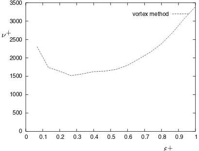
Figure 3. Spectral numerical viscosity of the VIC method withM4.

5.

Choice and optimization of parameters

Interpolation kernels are a key element of the vortex-in-cell method. In the first part of this section we analyze the spectral numerical viscosity associated with well-established interpolation kernels when used within the VIC method. In the second part, a new kernel for implicit LES is derived from the linear combination of standard kernels. Pursuing this natural approach, the weights are parameters of an implicit sub-grid scale model.

Figure 2 shows the results obtained with M4 and Λ3. The values of the numerical spectral viscosity are acceptable, but the shapes do not match with the theoretical curve. Particularly, the numerical viscosity decreases at the last wave numbers, whereas turbulence theory requires an increase of the eddy viscosity. We also notice that the values of the spectral viscosity are smaller than expected at low wave numbers. However, this ought to be less important for the scheme’s ability to model SGS effects.

At this point, we decide to try to built an implicit SGS model by using a linear combination of the interpolation functionsM4 and Λ3, potentially corrected at large wave-numbers by a small contribution of M4

K=c1M4+c2Λ3+c3M4 . (22)

Consistency requires_ici= 1, i.e. two parameters,c2andc3, are available for SGS modeling andc1= 1−c2−c3.

-0.4 -0.2 0 0.2 0.4 0.6 0.8

0 0.1 0.2 0.3 0.4 0.5 0.6 0.7 0.8 0.9 1 reference vortex method (a) ν+ ξ+ -0.4 -0.3 -0.2 -0.1 0 0.1 0.2 0.3 0.4 0.5 0.6 0.7

0 0.1 0.2 0.3 0.4 0.5 0.6 0.7 0.8 0.9 1 reference vortex method (b) ν+ ξ+ -0.4 -0.3 -0.2 -0.1 0 0.1 0.2 0.3 0.4 0.5 0.6 0.7

0 0.1 0.2 0.3 0.4 0.5 0.6 0.7 0.8 0.9 1 reference vortex method (c) ν+ ξ+ 0.2 0.3 0.4 0.5 0.6 0.7 0.8 0.9 1

0 0.1 0.2 0.3 0.4 0.5 0.6 0.7 0.8 0.9 1 reference vortex method (d)

ν+

ξ+

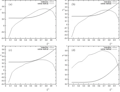
Figure 4. Spectral numerical viscosity of the vortex method with a combination ofM₄, Λ₃and M4with respective coefficients (a)c= (0.5,0.5,0.0), (b)c= (0.6,0.4,0.0), (c)c= (0.7,0.3,0.0), and (d)c= (0.599,0.4,0.001).

Figure 4 shows the numerical spectral viscosity evaluated for several combinations ofM4 and Λ3, withoutM4. The result obtained with the combinationc= (0.7,0.3,0.0) is not satisfactory, because the numerical viscosity becomes negative at the last wave number andc= (0.5,0.5,0.0) is too dissipative. Hence, the optimum value for c2 is bounded by 0.3 < c2 < 0.5. The combinationc = (0.6,0.4,0.0) gives good results in the range of normalized wave-numbers ξ+ = 0.3...0.8. We thus decide to consider this as our best combination of M4 and Λ3.

We do not claim that (0.6,0.4,0.0) is the optimum solution to the given problem. For the purpose of the present study, however, this set of parameters is sufficiently close to the optimum. In order to determine an optimum solution to a nonlinear problem, systematic (and time-consuming) optimization strategies, e.g. an evolutionary optimization algorithm as employed by Adamset al. [1], are required.

6.

Numerical results

For an a posteriori validation of the implicit SGS model provided by the VIC method with the selected linear combination of interpolating kernelsM4 and Λ3 we perform LES of a 2D Taylor-Green vortex, of a 3D Taylor-Green vortex, and of decaying isotropic turbulence.

All simulations presented in this section are carried out in a (2π)3-periodic computational domain, discretized with a uniform cartesian grid of 32×32×32 cells, and the same number of particles. For time advancement, we use an explicit fourth-order Runge-Kutta scheme.

6.1.

Two-dimensional Taylor-Green vortex

The two-dimensional Taylor-Green vortex in a periodic domain has an analytical solution that reads

u1 = −√acos(kx1) sin(kx2) exp(−(2k)2t/Re) u2 = √asin(kx1) cos(kx2) exp(−(2k)2t/Re)

u3 = 0 (23)

withu1, u2, u3 being the components of the velocity vector. The parameters of our numerical simulation are k= 1,Re= 1, anda= 0.0016.

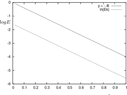
The analytical decay exponent of the kinetic energy is −4t/Re. Figure 5 shows the line y =−4t and the logarithm of the kinetic energy evaluated from the numerical simulation. It is observed that the numerical results are in excellent agreement with the theoretical prediction. The vortex is well-resolved by 323particles.

-6 -5 -4 -3 -2 -1 0

0 0.1 0.2 0.3 0.4 0.5 0.6 0.7 0.8 0.9 1 y = - 4t

ln(Ek)

logE

t

Figure 5. Decay of the kinetic energy of the 2D Taylor-Green vortex.

0 2 4 6 8 10 0

0.005 0.01 0.015

∂E ∂t

t

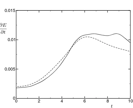
Figure 6. Rate of kinetic-energy dissipation for LES of the 3D Taylor-Green vortex at Re = 400. −−−−−−−DNS data from Ref. [2],−−−−implicit LES with VIC method.

6.2.

Three-dimensional Taylor-Green vortex

The 3D viscous Taylor-Green Vortex (TGV) characterized by the initial data

u1 = 0

u2 = cos(kx1) sin(kx2) cos(kx3)

u3 = −sin(kx1) cos(kx2) sin(kx3) (24)

has no analytical solution. It was subject to a large number of investigations since it was supposed that the initially laminar flow develops singularities atRe→ ∞. Numerically, no blow-up has been observed, but there is still no proof [10].

In order to assess the quality of LES using the VIC method, the characteristic growth and decay of the dissipation rate is compared with DNS data. The DNS of Brachetet al.[2] provides detailed reference data for the 3D Taylor-Green vortex. These spectral DNS exploit spatial symmetries of the TGV to reduce the effective computational cost by a factor of 8. It was therefore possible to resolve Reynolds numbers up to Re = 5000 on a grid of 8643 modes. For the present LES, spatial symmetries are not imposed, i.e. the (2π)3-periodic computational domain contains 8 counter-rotating vortices andk= 1 in eq. (24).

Using a grid of 323 cells, a fair comparison of LES with Brachet’s DNS is possible for Reynolds numbers Re = 100, Re = 200, and Re = 400. Figure 6 shows the dissipation rate for LES and DNS at Reynolds number Re = 400. LES and DNS compare reasonably well. Note that the resolution requirement of the DNS is two orders of magnitude higher than that of the LES. These results for the 3D Taylor-Green vortex confirm that the PIC method does not affect the growth of the instability modes of the initially laminar flow and does provide sufficient SGS dissipation to stabilize the simulation during the ensuing quasi-turbulent stage.

6.3.

Comte-Bellot - Corrsin experiment

1 10 10-4

10-3 10-2 10-1

(a)

E(ξ)

ξ 1 10

10-4 10-3 10-2 10-1

(b)

E(ξ)

ξ

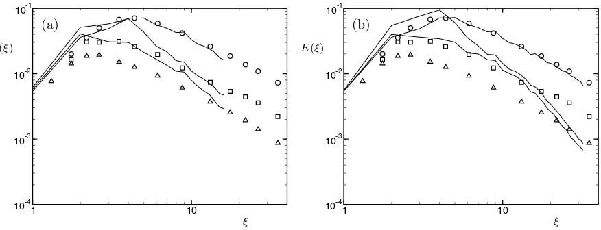
Figure 7. Instantaneous 3D energy spectra for LES with the VIC method of the Comte-Bellot – Corrsin experiment. (a) LES with 323 cells/particles, dt = 0.03. (b) LES with 643 cells/particles, dt = 0.015. Symbols represent experimental data of Ref. [5] ( t = 42 , t= 98 and t= 171), solid lines denote the present LES.

In the simulation this flow is modeled as decaying turbulence in a (2π)3-periodic computational domain. Based on the Taylor hypothesis the temporal evolution in the simulation corresponds to a downstream evolution in the wind-tunnel experiment with the experimental mean-flow speed which is approximately constant. The energy distribution of the initial velocity field is matched to the first measured 3D energy spectrum of CBC. The SGS model is verified by comparing computational and experimental 3D energy spectra at later time instants which correspond to the other two measuring stations. For more details, particularly with respect to non-dimensionalization and initial-data generation, we refer to [14].

In this test case a correct representation of the energy containing range of the spectrum is as important as the proper modeling of the subgrid stresses. The present VIC method does not satisfactorily meet these requirements. The large-scale turbulence decays too slowly, whereas the method over-predicts the dissipation at the smallest resolved scales, see fig. 7a. The situation does not change when the number of particles is increased. Figure 7b shows results from a LES with 64×64×64 cells and the same number of particles.

7.

Conclusions

We have proposed a new approach to design interpolation kernels assigned to the specific use in the implicit large-eddy simulation (LES) of turbulent flows. In implicit LES the subgrid-scale model is implicitly contained within the discretization. An explicit computation of model terms therefore becomes unnecessary.

The numerical truncation error of the vortex-in-cell method is analyzed a-posteriori through the effective spectral numerical viscosity in simulations of three-dimensional isotropic turbulence. The interpolation kernels used for velocity-smoothing and re-meshing were identified as the most relevant components affecting the shape of the spectral numerical viscosity. Turbulence theories, such as EDQNM [3, 19], define strict requirements for the spectral eddy viscosity to be met by a SGS model. The inherent eddy viscosity of standard kernels is found to be insufficient.

for implicit LES to only a limited extent. Simulations of different Taylor-Green vortices give encouraging results, whereas the predictions for decaying isotropic turbulence shows room for improvement.

The investigated kernels consume no extra computational resources because the linearity of the discretization is preserved. However, this advantage can also be considered as a major drawback. Explicit SGS modeling has clearly demonstrated the benefits of dynamic, solution-adaptive strategies, which correspond to non-linear discretization schemes in implicit LES.

Future interpolation kernels will incorporate more degrees of freedom allowing for an improved agreement of the spectral numerical viscosity with turbulence theory. Our results suggest that a solution-adaptive strategy, e.g. through local time-stepping or nonlinear weight functions, may be required.

References

[1] N.A. Adams, S. Hickel, and S. Franz. Implicit subgrid-scale modeling by adaptive deconvolution.J. Comp. Phys., 200:412–431, 2004.

[2] M.E. Brachet, M. Meneguzzi, A. Vincent, H. Politano, and P.-L. Sulem. Numerical evidence of smooth self-similar dynamics and possibility of subsequent collapse for three-dimensional ideal flow.Phys. Fluids, 4:2845–2854, 1992.

[3] J.-P. Chollet. Two-point closures as a subgrid-scale modeling tool for large-eddy simulations. In F.Durst and B.E. Launder, editors,Turbulent Shear Flows IV, pages 62–72, Heidelberg, 1984. Springer.

[4] J.P. Christiansen. Numerical simulation of hydrodynamics by the method of point vortices.J. Comput. Phys., 13:363–379, 1973.

[5] G. Comte-Bellot and S. Corrsin. Simple Eulerian time correlation of full and narrow-band velocity signals in grid-generated ‘isotropic’ turbulence.J. Fluid Mech., 48:273–337, 1971.

[6] G.-H. Cottet. Artificial viscosity models for vortex and particle methods.J. Comput. Phys., 127:299–308, 1996.

[7] G.-H. Cottet and P.D. Koumoutsakos.Vortex methods: Theory and Practice. Cambridge University Press, Cambridge, UK,

2000.

[8] G.-H. Cottet and L. Weynans. Particle methods revisited: a class of high-order finite-difference methods.C. R. Acad. Sci. Paris, Ser. I, submitted( ): , 2006.

[9] J. A. Domaradzki and D. D. Holm. Navier-Stokes-alpha model: LES equations with nonlinear dispersion. In B. Geurts, editor,

Modern Simulation Strategies for Turbulent Flow, pages 107–122. R. T. Edwards, 2001. [10] U. Frisch.Turbulence. Cambridge University Press, 1995.

[11] S. Ghosal. An analysis of numerical errors in large-eddy simulations of turbulence.J. Comput. Phys., 125:187–206, 1996. [12] F.F. Grinstein, L.G. Margolin, and W.G. Rider, editors.Implicit Large Eddy Simulation: Computing Turbulent Flow Dynamics.

Cambridge University Press, Cambridge, UK, 2007.

[13] W. Heisenberg. Zur statistischen Theorie der Turbulenz.Z. Phys. A, 124:628–657, 1948.

[14] S. Hickel, N.A. Adams, and J.A. Domaradzki. An adaptive local deconvolution method for implicit LES. J. Comp. Phys., 213:413–436, 2006.

[15] S. Hickel, T. Kempe, and N.A. Adams. On implicit subgrid-scale modeling in wall-bounded flows. In Proceedings of the

EUROMECH Colloquium 469, pages 36–37, Dresden, Germany, 2005.

[16] S. Hickel, T. Kempe, and N.A. Adams. Implicit large-eddy simulation applied to turbulent channel flow with periodic con-strictions.Theoret. Comput. Fluid Dynamics, 2006. (submitted).

[17] A. Kravchenko and P. Moin. On the effect of numerical errors in large-eddy simulation of turbulent flows.J. Comp. Phys., 130:310–322, 1997.

[18] A. Leonard. Energy cascade in large eddy simulations of turbulent fluid flows.Adv. Geophys., 18A:237–248, 1974. [19] M. Lesieur.Turbulence in Fluids. Kluwer Academic Publishers, Dordrecht, The Netherlands, 3 edition, 1997. [20] J. J. Monagan. Extrapolating B splines for interpolation.J. Comput. Phys., 60:253–262, 1985.

[21] M. Ould-Salihi, G.-H. Cottet, and M. El Hamraoui. Blending finite-difference and vortex methods for incompressible flow computations.SIAM J. Sci. Comp., 22:1655–1674, 2000.