Lecture14-ControllerDesignviaRootLocus

(1)

Page : 1 EE406 Control Systems Lecture 13 : Root Locus

UCSI University Faculty of Engineering

Kuala Lumpur, Malaysia Department of Mechatronics

Lecture 14

Controller Design via Root Locus

Mohd Sulhi bin Azman Lecturer

Department of Mechatronics UCSI University

[email protected]

1 August 2011

Contents

• Compensation and design of compensators

• Introduction to PID control

(2)

Compensation

• A closed-loop system is usually an unstable system. Hence, because it is unstable, there must be some kind of compensators than can compensate the stability of a closed loop system.

• Compensators are used to alter the output response of a system in order to accommodate to the set of desired criteria. This is achieved by introducing additional poles and/or zeros to the system transfer function.

• Sometimes, the word regulator or correction is used instead of the word compensator.

Compensation

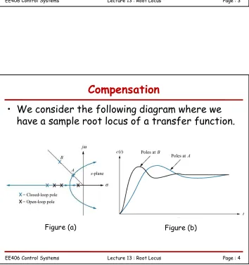
• We consider the following diagram where we

have a sample root locus of a transfer function.

(3)

Compensation

• In the previous diagram, we assume that the desired output that we want is at point B. However, we note that currently, our output is at A. And we further note that at both points A and B, we desire a system with a “nice” percent overshoot and settling time.

• When we change the location of the root from point A to point B, the system response is speed-up, and

interestingly, the percent overshoot is not affected.

• When we want to change from point A to point B, we can’t simply adjust the gain of the system; rather, we need to introduce additional poles and/or zeros.

Compensation

• The introduction of additional zeros and/or poles will speed-up the response of the system.

• When we introduce additional poles/zeros, we are

actually improving the transient response of the system, as well as reducing the steady-state errors.

• Additional poles will eventually improve the steady-state characteristics, while additional zeros will improve the transient response.

(4)

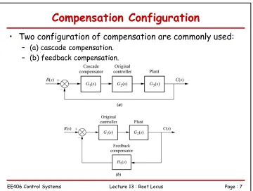
Compensation Configuration

• Two configuration of compensation are commonly used:

– (a) cascade compensation. – (b) feedback compensation.

Compensator Design

• There are two (2) types of compensators:

– (a) pure integration (1/s) – (b) pure differentiation (s).

• Other types of compensators include a lead and lag compensator system.

Ideal compensators.

Figure (a) : Phase Lead Figure (b) : Phase Lag

(5)

Compensator Design

• We shall look at two ways of designing a

compensator. The compensators will generally:

– (1) improve the steady state error, by means of adding additional poles or integrators.

– (b) improve the transient response by means of adding additional zeros or differentiators.

COMPENSATOR DESIGN (1)

(6)

Compensator Design (1)

• This method improves the steady-state error.

• It uses:

– (a) ideal integral compensation.

• Uses a pure integrator to place an open-loop, forward path pole at origin.

• This will increase the system type and reduce the steady-state error to zero.

– (b) integral compensation • Does not use pure integrator.

• It place the poles near the origin. However, this won’t bring the steady-state error to zero, but still, you get a considerable reduction in error.

Design of Ideal Integral Compensation

• Consider the following un-compensated system:

Here, this system has a desirable transient response which is

generated by the closed-loop poles at A.

In this case, we see that the angular contribution to this pole is 180°.

(7)

Design of Ideal Integral Compensation

• As was said in the previous slide, adding a pole alone will alter the shape of the root locus.

• And worst, the “new” root locus does not go through point A. And this is what we do not want.

• Thus, to solve this problem, we add a zero close to the pole at the origin. See the diagram in the next slide.

Design of Ideal Integral Compensation

• By adding extra zeros, the angular contribution of the poles and zeros cancel out.

• And furthermore, point A is now on the root locus. And we note that the system type has been increased.

(8)

Design of Lag Compensation

• We note that the design of ideal integral compensation involves the use of pure integrator. Now, this time, we will not use pure integrator. We will use poles and zeros that are close to the origin, but not necessarily on the origin.

• Let us consider a type 1 uncompensated system which is shown below:

Design of Lag Compensation

• The above system can be improved by adding a compensator

transfer function in the feed-forward section of the loop:

(9)

Design of Lag Compensation

• How will this effect on the transient response of the system? And how will this effect on the required gain, K? Let us consider the root locus plot of the system:

(Uncompensated) (Compensated)

Design of Lag Compensation

• We establish here that:

– after the additional of compensated zeros and pole in Figure (b) of the previous slide, the angular contributions are approximately zero, and therefore, point P is still approximately on the location of the root locus. – the gain K is still the same for both compensated and

uncompensated system.

• It can be concluded that in order to keep the transient response unchanged, the compensator pole and zero must be close to each other; and the pair must also be closed to the origin.

(10)

COMPENSATOR DESIGN (2)

Improving the transient response

Compensator Design (2)

• Recall that differentiators are the zeros in the

s-domain.

• This technique will improve the transient

response of the system. Usually, we wanted a

desirable percent overshoot and shorter

settling time.

• There are two (2) techniques:

(11)

Design of Ideal Derivative Compensation

• The ideal derivative is a pure differentiator.

• In designing an ideal compensation system, a pure differentiator is added to the forward path of the feedback control system. The reason for this is ensure that the closed-loop pole is placed on the root locus.

• We have to remember that we wanted to design a system with better transient response. Therefore, we need to have a dominant pole of the characteristic equation. A dominant pole of the characteristic equation is usually a complex root.

Recall – Dominant Poles

• A dominant pole is a complex root of characteristic equation.

• The general form of a dominant pole is given as follows, along with the sketch of the dominant pole:

2

1,2 n n

1

(12)

• Consider the following root locus plot of an uncompensated system.

• Pay close attention to the location of the open-loop poles and the closed loop poles.

( 1)( 2)( 5)

K OLTF

s s s

=

+ + +

Design of Ideal Derivative Compensation

• We can improve the

transient response of this system by adding a compensator zero at -2.

• Now, pay attention to the location of the open-loop pole and the closed-loop poles.

• The closed-loop poles is now a dominant pole, hence better transient response.

( 2) ( )

( 1)( 2)( 5)

c

K s G s

s s s

+ =

(13)

Design of Ideal Derivative Compensation

• We now add a

compensator zero at -3. Hence:

• And we now look at the location of the poles (open-loop and the closed-loop).

( 3) ( )

( 1)( 2)( 5) c

K s G s

s s s

+ =

+ + +

• We now add a

compensator zero at -4. Hence:

• And we now look at the location of the poles (open-loop and the closed-loop).

( 4) ( )

( 1)( 2)( 5) c

K s G s

s s s

+ =

(14)

Design of Ideal Derivative Compensation

• Let us compare the predicted characteristics of the system described in previous slides:

• The following observations can be made:

– Each of the compensated cases has dominant poles with the same damping ratio as the uncompensated system. Therefore, we expect to have same percent overshoot for all cases.

– The compensated, dominant, closed-loop poles with more negative real parts will have the shortest settling time.

– The value of the imaginary part of the compensated system is larger. Thus, all compensated system will have smaller peak time compared to the uncompensated system.

(15)

Design of Ideal Derivative Compensation

• Time response of compensated and

uncompensated systems:

Design of Lead Compensation

• In the design of lead compensation system, we make use of both compensator pole and zero.

• We note here that if the pole is farther from the imaginary axis than the zero, the angular contribution will still be positive, and thus approximate an equivalent single zero.

(16)

Design of Lead Compensation

• The following is the geometry of lead compensation.

2 1 3 4 5 (2k 1)180

θ θ θ θ θ− − − + = +

2 1 c

θ θ θ− = Angular contribution:

Compensator angle:

Design of Lead Compensation

(17)

PID Control

• PID control is the most widely used controller in the field of industrial automation.

• PID is an abbreviation of: – Proportional (P), – Integral (I), and – Derivative (D).

• So far, in the previous slide, we have indirectly discussed the concept of PID control scheme.

• A PI control scheme is actually the ideal integral

compensation system, while a PD control scheme is actually the ideal derivative compensation system.

PID Control

• The defining equation for a PID control scheme can be expressed in time domain as follows:

• Taking a forward Laplace transform yield:

where K_p, K_iand K_dare called the proportional gain, integral gain and derivative gain respectively. The variable e(t) or E(s) is known as the error signal.

( )

c p i d

de t

G t

K e t

K

e t dt

K

dt

=

+

∫

+

( )

i

( )

c p d

K

G s

K E s

E s

K s E s

s

(18)

PID Control

• The block diagram of a PID control scheme is

shown as follows:

PID Control

• We consider a special case of PI and PD control.

• As discussed, a PI control is the ideal integral compensation design. A PI control scheme is also obtained when the derivative gain (K_d) is set to equal zero: K_d=O.

(19)

PI controller

• Since in PI control scheme, we set K_d=O, then we obtain the following transfer function for a PI controller:

• As discussed, the PI controller is used to reduce the steady-state error.

(

)

(

)

( )

i p i

c p

p i p p c

K s

K

G s

K

s

K

s

K K

K

s

z

s

+

=

+

=

+

=

PD controller

• Since in PD control scheme, we set K_i=O, then we obtain the following transfer function for a PD controller:

• As discussed, the PD controller is used to improve the transient response of a system, especially the percent overshoot and the settling time.

(

)

(

)

( )

c p d d p d d c

(20)

Phase Compensators

• There are two (2) type of phase compensators:

– (a) phase lag compensator.

– (b) phase lead compensator

all of which has been indirectly discussed.

Phase Lag Compensator

(21)

Phase Lead Compensator

• It is used to improve transient performance.

Example 1

• A control system is described by the following block diagram:

The transfer function of the plant is:

Design a controller (compensator) so that the closed-loop pole has an overshoot of 5% and a settling time of 2 seconds.

10

( )

(

1)

G s

s s

=

(22)

Solution to Example 1

• According to the question, we desire:

%OS = 5% = 0.05 Ts = 2 seconds

• From these given values, we can calculate the damping ratio and the natural frequency.

• Hence:

(

)

(

)

(

)

2 2 2 2

ln % / 100 ln 0.05

ζ 0.69 0.7

ln % / 100 ln 0.05 OS OS π π − − = = = + + ≃

4 4 4

2.86 3 (0.7)(2) s n n s T T ω ζω ζ = ⇒ ₌ ₌ ₌ _≃

Solution to Example 1

• Next, we form a second order characteristic equation:

• Solving the above characteristic (quadratic) equation yields a desired dominant poles:

• Now, we look at the given plant transfer function. The transfer function consists of integrators (having a pole at s=0 and s=-10). Therefore, a suitable controller (compensator) would be a PD controller because of the fact that PD will improve the transient response of the system.

2 2 2 2 2

2

ζ

_n _n

2(0.7)(3)

(3)

4.2

9

s

+

ω

s

+

ω

=

s

+

s

+

=

s

+

s

+

1,2

2.1

2.14

2

(23)

Solution to Example 1

• The general transfer function for a PD controller is described as follows:

• Recall that a PD controller is an example of a leading system in which we introduce an extra zero that could provide a better transient response. And in a leading system, |z| < |p|.

• First, we sketch the pole-zero map of the plant transfer function (shown in the next slide).

( ) ( )

c p d d

G s = K +K s= K s+z

p d

z =K K Where:

• Note:

– We place the compensator zero anywhere on the s-plane for as long as we meet the condition that |z| < |p|. Or put it in another way, |p| > |z|. Therefore, in here we see that the zero must be to the left of all the pole of the plant transfer function.

– Point A is the location of the dominant poles which give the desired transient response. In this case, at point A, s = -2 ±j2.

(24)

Solution to Example 1

-1 zc

A

θ1

θ2

θc

j2

-2

• Let us calculate the angular contribution of θ₁and θ₂.

• Note that in order for the dominant poles (A) to be located in the root locus, each poles and zeros must contribute some angles to point A.

1 1

2

180 tan 135

2

θ ₌ ₋ −  ₌

   

1 2

2

180 tan 116.65 117 1

θ ₌ ₋ −  ₌

   

(25)

Solution to Example 1

• Now, the contribution of the compensator angle can be calculated by using the following formula:

• Normalizing the angle gives:

( )

(

)

180 0 135 117 180 180 252 432

c zeros poles c

c

θ θ θ

θ θ + − = + − + = = + =

∑

432 360 72

c

θ = − =

• Now, once we know the angle, what do we do next? We refer to the pz-map in the previous slide. What we did just now was to calculate the angular location of the compensator zero. We now wish to determine the location of the compensator zero on the pz-map.

72° x 2 2 tan 72 2 0.65 0.7 tan 72 x x = = = ≃

2 0.7 2.7 3

c

z = − − = − ≃−

From trigonometry:

(26)

Solution to Example 1

• What we did so far was to calculate the location of the angular contribution of the compensator zero. Once we know how to calculate the angular contribution, we can then use basic and simple trigonometry to determine the exact (or approximate) location of the compensator zero.

• Now, we know for a fact that z_c = -3. We now proceed to calculate the gains K_p and K_d. To do this, we have to use the magnitude condition:

dominant poles

( ) ( ) 1

c plant _s

G s G s

=

⋅ =

Solution to Example 1

• We next do the following:

( )

2 2

2 2 2 2 10

3 1

( 10)

1

2 2 3 1

( 2 2)( 2 2 10)

1 2

1 ( 2 2) (8 2)

1 2

1 ( 2) 2 8 2

(27)

• We state that the computed values of K_pand K_dare 3 and 10 respectively. Since the gain of the plant transfer function is K=10, then we divide the values of 3 and 10 by 10, hence yielding:

K_p= 0.3 K_d = 1

• Therefore, the compensator transfer function is:

( ) ( ) 0.3

c d

G s =K s+ = +z s

Next Step

• Textbook reference : Chapter 9.

• Homework 12 has been posted on the course

website. Attempt them. You do not have to

submit Homework 12 as it will not be graded.