http://www.sciencepublishinggroup.com/j/ajpa doi: 10.11648/j.ajpa.20190701.11
ISSN: 2330-4286 (Print); ISSN: 2330-4308 (Online)
Motion and Interaction of Envelope Solitons in Schrödinger
Equation Simulated by Symplectic Algorithm
Lai Lianyou
1, 2, *, Xu Weijian
21
College of Information Engineering, Jimei University, Xiamen, China
2College of Mechanical Engineering and Automation, Huaqiao University, Xiamen, China
Email address:
*
Corresponding author
To cite this article:
Lai Lianyou, Xu Weijian. Motion and Interaction of Envelope Solitons in Schrödinger Equation Simulated by Symplectic Algorithm.
American Journal of Physics and Applications. Vol. 7, No. 1, 2019, pp. 1-7. doi: 10.11648/j.ajpa.20190701.11
Received: November 18, 2018; Accepted: December 14, 2018; Published: January 21, 2019
Abstract:
The expression of Gaussian envelope soliton in Schrödinger equations are given and proved in this paper. According to the characteristics of the Gauss envelope soliton, further proposed that the interaction between Gaussian envelope solitons exists in Schrödinger equation. The symplectic algorithm for solving Schrödinger equation is proposed after analysis characteristics of Schrödinger equation. First, the Schrödinger equation is transformed into the standard Hamiltonian canonical equation by separating the real and imaginary parts of wave function. Secondly, the symplectic algorithm is implemented by using the Euler center difference method for the canonical equation. The conserved quantity of symplectic algorithm is given, and the stability of symplectic algorithm is proved. The numerical simulation experiment was carried out on Schrödinger equation in Gauss envelope soliton motion and multi solitons interaction. The experimental results show that the proposed method is correct and the symplectic algorithm is effective.Keywords:
Schrödinger Equation, Soliton, Symplectic Algorithm, Optical Communication1. Introduction
The research and application of solitons have gone deep into various fields, such as mathematics, fluid dynamics, nonlinear electromagnetism, optical fiber communication, solid state physics and so on. The definition of soliton is not the same in all research fields. Scholars of pure theory, such as mathematicians, define the soliton very strictly. From the mathematical point of view, the soliton is a stable, energy limited undispersed solution of some nonlinear partial differential equations, that is, it can always keep the wave and velocity unchanged. Scholars who value applications, such as some applied physicists, are more relaxed about the definition of soliton. Physicists believe that as long as the energy of the wave is limited and is distributed in a limited space or time range, even if the wave changes during the propagation process, such as the high order optical soliton in the optical fiber, they are also called soliton. There are many forms of solitons, such as bell shaped soliton, ring soliton, twisted soliton, enveloping soliton, anti soliton, sentry soliton,
respiratory soliton, etc.
Soliton has experienced a historical process from discovery to establish mathematical model and application. In 1834, John Scott Russell accidentally discovered the soliton waves in the canal. In 1895, D J Korteweg and De Vries proposed the KdV equation of one-way wave propagation in fluids, theoretically proved the existence of solitons. In 1955, Enrico Fermi, John Pasta and Stan Ulam confirmed the existence of solitons using computer numerical experiments. In 1962, Perring and Skyrme used Sine-Gordon equation to study the basic particles. The calculation results show that the soliton is spread out, even if the two soliton collision also still maintain the original shape and speed. In 1965, M. D. Kruskal and N. Zabusky used numerical simulation method to study the nonlinear interaction process of the soliton collision in plasma. The results further confirmed that the soliton wave remains constant shape and speed after the collision. At present, the soliton research has entered the application stage, especially the application of optical soliton in optical fiber communication field has achieved a lot of results [1-4].
equation. For the interaction process of solitons, it can be observed, verified and tested by numerical simulation [5-6]. There are many methods of numerical simulation, and the most commonly used method is the finite difference method. Symplectic algorithm is a numerical algorithm suitable for Hamiltonian system equations.
In 1984, Feng Kang [7] made a presentation report entitled "difference scheme and the symplectic geometry", first proposed the symplectic geometry algorithm for Hamiltonian system, in the Beijing conference of differential geometry and differential equation computation of partial differential equations. Since then, Feng Kang and his team system [8-9] developed this algorithm in. The symplectic algorithm has obvious advantages compared with then on symplectic algorithm when the numerical calculation for the Hamiltonian systems. Because of maintaining the symplectic structure, the symplectic algorithm makes the numerical calculation of each step be a symplectic transformation, eliminate the artificial dissipation introduced non symplectic algorithm in the calculation process. Therefore, it has the long time tracking ability and high stability for the evolutionary computation [10-15].
The Schrödinger equation belongs to Hamiltonian system, it's mathematical framework is the theory of Hilbert spaces. Calculate the object of symplectic algorithm is a Hamiltonian system, it's mathematical framework is symplectic geometry. Therefore, the transform is necessary from the Schrödinger's equations to the symplectic algorithm. The Schrödinger equation is complex. If the real part and the imaginary part of the wave function ware regarded as the generalized coordinates and generalized momentum. The Schrödinger equations can be written in standard form canonical equations of Hamilton system.
In the Schrödinger equation, the researchers are concerned with the mode square (wave packet) of the wave function instead of the direct solution of the Schrödinger equation.
Because the direct solution of the Schrödinger equation is a conjugate complex number in pairs which physical meaning is unknown, but the wave packet is a real number which physical meaning is clear.
The researching objects of this paper is the Gauss envelope soliton in Schrödinger equations, their motion and interaction process, using the method of combining the analytical method and symplectic algorithm. On the one hand, the correctness of symplectic algorithm will be verified, on the other hand the characteristics of solitons motion and interaction will be also verified by the numerical simulation using symplectic algorithm.
2. Analytical Solutions and Interaction of
Envelope Solitons in the Schrödinger
Equation
The one-dimensional stationary Schrödinger equation is
shown in (1).
( )
2 2( ) ( )
2
,
i = ,
2
x t
V x x t
t m x
ψ ψ
∂ − ∂ +
∂ ∂
ℏ
ℏ (1)
Where,i is the imaginary symbol; ℏ=h2π, h is the Planck constants, m is the quantum quality,ψ( )x t, is the wave function, V x( ) is the potential function. x is the position of quantum which is one-dimensional (1D), 2D or 3D.
2.1. The Schrödinger Oscillator Equation
In theory, any potential function can be approximation using the parabolic at the nearby of minima in the vicinity can use according to the Taylor series expansion principle. In practice, any vibration, as long as the amplitude is small enough, can be seen as simple harmonic vibration.
In the case of harmonic vibration, potential function is shown in (2).
( )
1 2 22
V x = mωx (2)
Where,ω is the resonant frequency.
The Schrödinger equation (1) can be written to the form such as (3) when potential function is the harmonic oscillator function.
( )
2 2( )
2 2 2
1
i , ,
2 2
x t m x x t
tψ m x ω ψ
∂ = − ∂ +
∂ ∂
ℏ
ℏ (3)
2.2. The Envelope Soliton Solution of Schrödinger Harmonic Oscillator Equation
The Schrödinger harmonic oscillator equation has the envelope soliton solution. The envelope soliton solutions must satisfy two conditions: A. The wave function satisfies the Schrödinger harmonic oscillator equation as (3); B.The wave function does not change with time which always keeps the properties of soliton. The (4) is a envelope soliton solution of Schrödinger harmonic oscillator equation.
( ) 1 4 2 2
(
2 i)
i i, exp 1 2
2
t t
m m a t
x t x e axe
m
ω ω
ω ω
ψ = − + + − + − −
π π
ℏ
ℏ ℏ (4)
Where,ais a real number presenting the length scale. The condition A is proved as the following:
First,
( )
x t,tψ ∂
∂ , xψ
( )
x t,∂
∂ , ( )
2
2 x t,
t ψ
∂
∂ are calculated such as (5), (6), and (7).
( )
, 2(
2i 2i)
i 2( )
i( )
,2 2
t t
m a
x t e ax i e x t
t m
ω ω
ω
ψ ω − ω − ψ
∂
= − − + − −
∂
ℏ
ℏ (5)
( )
(
i)
( ), m t ,
x t x ae x t x
ω
ω
ψ − ψ
∂
= − −
∂ ℏ (6)
( ) 2
(
)
( )2
2 i 2 2i
2 , 2 ,
t t
m m
x t x axe a e x t
x
ω ω
ω ω
ψ − − ψ
∂ = − + − +
The Schrödinger harmonic oscillator equation will be established if (5) and (7) substitute into (3).
The condition B is proved as the following:
The wave packet is shown in (8) calculated by wave function (4).
( )
2(
)
2, m exp m cos
x t ω ω x a t
ψ = − − ω
πℏ ℏ (8)
The (8) can be transformed into (9).
( ) ( )
2 2 2
2
1 ,
2
x
x t e
µ σ
ψ
πσ
− −
= (9)
Where,
cos
a t
µ= ω (10)
2m
σ= ℏω (11)
From equation (9), (10) and (11) can be seen: (1) the shape of wave packetψ
( )
x t, 2is invariant and Gaussian; (2) the center µ of wave packet is cosine with the amplitude aand the oscillating frequencyω; (3) The wave packet width is determined by σ, and its size is inversely proportional to ω . σis smaller, wave packet more narrow, kurtosis larger, the corresponding oscillation frequency ωlarger, i.e. motion speed greater.In the Hamilton system, the generalized coordinates and the generalized momentum are a pair of variables. The other observations variables can be to transform from them. Therefore the calculation of these two variables is very important. The Schrödinger equation belongs to the Hamilton system. The generalized coordinate and the generalized momentum are the variables of the probability type. Their mathematical expectations are usually.
The mathematical expectations of the coordinate is calculated by (12) are shown.
( )2
, d cos
x =
∫
−∞+∞xψ x t x=a ωt (12)Where,yis the intermediate variable, and y= −x acosωt.
From (12) it can be seen: the mathematical expectation of coordinate is the cosine wave with amplitude aand frequency
ω. The result is equal to the center position of the wave packet, which is the same (10). It reflected from a side that the wave packet maintains the symmetry of shape in movement. The mathematical expected is only equal to the value of the center if the wave packet is symmetric.
The mathematical expectation of momentum can be computed using (13).
d
sin d
x
p m ma t
t ω ω
= = − (13)
From (13) it can be seen that the mathematical expectation of momentum is the sine wave with the amplitude maωand the frequency ω.
The relationship between coordinate and momentum
mathematical expectation can be shown as (14) from (12) and (13).
(
)
2 2 2
2 1
x p
a + maω = (14)
According to the formula (14), the relationship between the coordinate and momentum mathematical expectation is elliptical. The trajectory is closed and elliptic in the phase space. In fact, it conclusion is consistent with the classical harmonic oscillator.
2.3. The Interaction Amongst Envelope Solitons in the Schrödinger Equation
According to the formula (4), the shape and motion of wave function are relevant with a and ω. In order to make the distinction of multi solitons, the wave function is expressed as
(x a, , ,t)
ψ ω in this paper.
When multiple solitons interact, their wave functions overlay as shown in (15).
( )
(
)
1
, , , ,
n
i i i i
x t x a t
ψΣ ψ ω
=
=
∑
,n=1,2,3⋯ (15)Where, n is the number of solitons.
The wave packet is the square of the wave function's models as shown in (16) when the multiple solitons interact.
( )
( )
2, ,
P x tΣ =ψΣ x t (16)
3. Symplectic Algorithm for Schrödinger
Equation
There are a variety of numerical solutions for the Schrödinger equation. Compared with other numerical methods, symplectic algorithm has outstanding advantages. It is shown that the algorithm can preserve the square of the model ψ
( )
x t, 2 conservation of the wave function. This advantage is the symplectic properties of symplectic algorithm for solving Schrödinger equation numerically.3.1. The Symplectic Algorithm for Schrödinger Equation
In (1), H is the Hamiltonian operator as shown in (17).
( )
2 2
= 2
2m x V x
∂
− +
∂
ℏ
H (17)
Therefore, (1) can be rewritten in matrix form as shown in (18).
i H
t
ψ ψ
∂ =
∂ (18)
Where,ψ is a complex matrix.
1
H=
In (3), H is the real matrix. H is replaced by central
difference 2
2
x
∂
∂ when it is numerical computated. so H is Hermite matrix.
According to [19], ψ can be written as the sum of real part and imaginary part, as shown in (20).
R i I
ψ ψ= + ψ (20)
The (21) is available after the (20) being substituted into (18).
(
R I) (
R I)(
R I)
i i H H i
t ψ ψ ψ ψ
∂ + = + +
∂ (21)
The (22) is available after expanding the (21).
R I
R I
i H iH
t t
ψ ψ ψ ψ
∂ −∂ = +
∂ ∂ (22)
The (23) is available after separating the real and imaginary parts of (22).
R I I
R
H t
H t
ψ ψ
ψ ψ
∂
=
∂
∂
= − ∂
(23)
The (23) can be abbreviated to (24) which is the Hamiltonian canonical form of Schrödinger equation.
R R
I I
0 0
H H t
ψ ψ
ψ ψ
∂ =
−
∂ (24)
The (24) can be abbreviated to (25).
t ∂ =
∂ Z
KZ (25)
Where,
R I
ψ ψ
=
Z (26)
0 0
H H
=−
K (27)
Since H is a Hermite matrix, (27) is established.
T= −
K K (28)
According to (28), it can be proved that K is a symplectic matrix, that is (29).
T + =0
K J JK (29)
Where,J is a symplectic unit matrix as shown in (30).
=
0
0
E J
E (30)
Where, E is a unit matrix.
For (26), there are some numerical calculation methods.
The Euler center format is symplectic, as shown in (31).
1 1
2
n n n n
t
+ − = ++
∆
Z Z Z Z
K (31)
The (31) can be deformed into (32) and (33).
(
)
1 1
2
n n n n
t
+ − = ∆ + +
Z Z K Z Z (32)
1
2 n 2 n
t t
+
∆ ∆
− = +
I K Z I K Z (33)
Where, I is a unit matrix.
Therefore, the iterative numerical solution of the symplectic scheme for (25) is shown in (34).
1
n+ = n
Z FZ (34)
Where,
1
2 2
t − t
∆ ∆
= − +
F I K I K (35)
3.2. The Symplectic Conservation Quantity in Schrödinger Equation
The general solution of the Schrödinger equation (18) is shown in the (36).
( )
exp iHt
ψ = − (36)
The (36) is numerical after discrete, and its iteration format is shown in (37).
( )
1 exp i
n+ = − ∆H t n
ψ ψ
ψ ψ
ψ ψ
ψ ψ (37)
In the (37), exp(− ∆iH t) is the time evolution matrix, and is
called G=exp(− ∆iH t). Because G is a complex exponential matrix, its determinant is 1, that is (38).
(
)
exp i t 1
= − ∆ =
G H (38)
After the comparison (34) and the (37), it can be found that F is equivalent to the time evolution matrix G . The difference is that Fis 2N×2N complex matrix, while G is
N×N complex exponential matrix.
Because F is a symplectic matrix, its determinant is 1 according to the properties of symplectic matrix.
1 =
F (39)
According to the formula (38) and (39), it can be found that the symplectic algorithm of the discrete form (34) maintains the properties of the Schrödinger equation. F =1 also shows that the symplectic scheme of (34) can guarantee the conservation of the form energy.
Therefore, ψR and ψI can be understood as generalized momentum and generalized coordinates. The form energy of symplectic algorithm is shown in (40).
( )
T( )
T R R I I1 1
2 2
n n n n n
E = ψψψψ ψψψψ + ψψψψ ψψψψ (40)
Where, n is the number of iterations. According to the formula (40), the form energy of the symplectic algorithm of (34) is the square of the modulus of wave function ψ( )x t, . It is in conformity with the physical meaning of the Schrödinger equation which is that the cumulative probability is a constant.
3.3. The Stability of the Symplectic Algorithm of the Schrödinger Equation
According to the formula (35), the F is a complex matrix. It can been seen that K is an anti Hermite matrix from (29). So there is the (41).
H
1 1
H
2 2 2 2
t − t t t −
∆ ∆ ∆ ∆
= − + = −
F I K I K I K I + K (41)
According to (35), F is the Cayley transformation of
2
t ∆
K . According to the characteristics of the Cayley
transformation, the available (42) is available.
1 1
2 2 2 2
t − t t t −
∆ ∆ ∆ ∆
= − + = + −
F I K I K I K I K (42)
Therefore, F−1 is shown in (43). 1
1 1
1 =
2 2 2 2
t t − − t t −
− = + ∆ − ∆ − ∆ + ∆
F I K I K I K I K (43)
After comparison (41) and (43), the (44) can be obtained.
H= −1
F F (44)
So, F is a unitary matrix. According to the properties of unitary matrix, the modulus of all the eigenvalues ofFare 1, that is:
1
i
λ = ,i=1, 2,3⋯ (45)
Since all the eigenvalues of F are not greater than 1, the (34) is always stable.
4. Simulation Experiment Results and
Analysis
This paper simulated the soliton motion and multiple solitons interaction using symplectic algorithm to numerical calculating. The calculation results using symplectic algorithm were compared with that using theoretical analytical solution. The simulation parameters are: Planck constant ℏ=1, quantum quality m=1, x range [−10,10],
0.2
x
∆ = , ∆ =t 0.02.
4.1. A Soliton Motion Process and Phase Trajectory
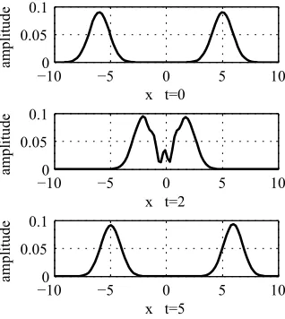
The wave function parameters are a=1, ω= π5. First, ( )x, 0
ψ was calculated by (4) as the initial wave function. Then, it was substituted into (35) and iterative calculate. The snap shots of wave package at t=0, 2,5 are shown in Figure 1.
Figure 1. The snapshotsof wave package.
As you can see from Figure 1: (1) The envelope soliton keep waveform unchanged during the movement; (2) After
5
t= , the soliton finished half a cycle, which arrived position
1
x= − from positionx=1. This results are consistent with the theoretical calculation equation (9).
In the case of a single envelope soliton motion, the energy n
E calculated according to the (40) is shown in Figure 2.
Figure 2. The form energy of a soliton.
As shown in Figure 2, the conserved quantity n
E of the symplectic algorithm has not changed in the numerical iterative calculation process, which is consistent with the theoretical analysis.
The coordinate mathematical expectation values x of a soliton motion change with time as shown in Figure 3.
Figure 3. x −t.
−100 −5 0 5 10 0.05
0.1
x t=0
a
m
p
li
tu
d
e
−100 −5 0 5 10 0.05
0.1
x t=2
am
p
li
tu
d
e
−100 −5 0 5 10 0.05
0.1
x t=5
am
p
li
tu
d
e
0 50 100 150 200 250 0.4999
0.5 0.5 0.5001
n
E
n
0 10 20 30 40
−1 0 1
t
<
x
As you can see from Figure 3: The coordinate mathematical expectation value x is a cosine wave, which the amplitude
and frequency are consistent with (12) of the theoretical calculation.
The relationship of single soliton motion between the coordinate mathematical expectation value x and the
momentum expectation value p is shown in Figure 4.
Figure 4. p − x .
As you can see from Figure 4: (1) The relationship between
x A and p is elliptical, which is consistent with the
theoretical calculation (14). (2) After 2000 times iterations, four cycle calculation, x − p still maintains a good numerical relations, which the four cycle trajectories completely overlap. It embodies the advantage of the symplectic algorithm.
4.2. Simulation of the Interaction Process of Multiple Solitons
4.2.1. Two Solitons Interaction
The wave function parameters are a1= −6 , a2=5 ,
1 2 5
ω ω= = π . First, ψ1(x a, 1,ω1, 0) and ψ2(x a, 2,ω2, 0) were
calculated using the (4). Second, ψ∑( )x, 0 was calculated by
the (15) as the initial wave function. Then, it was substituted into (34) and iterative calculate. The snap shots of wave package at t=0, 2,5 are shown in Figure 5.
Figure 5. The snapshots of two solitons interaction.
As you can see from Figure 5: (1) The shapes are invariant after the envelope solitons colliding each other. (2) After t=5, the solitons finished half cycle movement. The soliton 1 moved from position x= −6 to positionx=6; the soliton 2 moved from position x=5to positionx= −5.
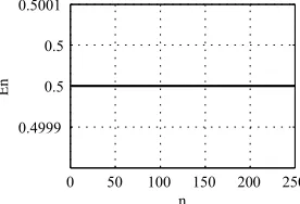
When the two envelope soliton moves, the energy n
E
calculated according to the (40) is shown in Figure 6.
Figure 6. The form energy of two solitons.
As shown in Figure 6, the conserved quantity n
E of the symplectic algorithm has not changed in the numerical iterative calculation process, which is consistent with the theoretical analysis.
4.2.2. Three Solitons Interaction
The wave function parameters area1= −7, a2= −1, a3=6,
1 2 3 5
ω ω= =ω = π . First, ψ1(x a, 1,ω1, 0) , ψ2(x a, 2,ω2, 0) and
( )
3 x a, 3, 3, 0
ψ ω were calculated using the (4). Second, ψ∑( )x, 0 was calculated by the (15) as the initial wave function. Then, it was substituted into (34) and iterative calculate. The snap shots of wave package at t=0, 2,5 are shown in Figure 7.
Figure 7. The snapshots of three solitons interaction.
As you can see from Figure 7: (1) The shapes are invariant after the envelope solitons colliding each other. (2) After t=5,
the solitons finished half cycle movement. The soliton 1 moved from positionx= −7 to positionx=7; the soliton 2 moved from position x= −1to positionx=1; the soliton 3 moved from position x=6to positionx= −6.
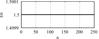
When the three envelope soliton moves, the energy n
E
calculated according to the (40) is shown in Figure 7.
−1 −0.5 0 0.5 1
−1 −0.5 0 0.5 1
<x>
<
p
>
−100 −5 0 5 10
0.05 0.1
x t=0
am
p
li
tu
d
e
−100 −5 0 5 10
0.05 0.1
x t=2
am
p
li
tu
d
e
−100 −5 0 5 10
0.05 0.1
x t=5
am
p
li
tu
d
e
0 50 100 150 200 250 0.9999
1 1.0001
n
E
n
−100 −5 0 5 10
0.05 0.1
x t=0
am
p
li
tu
d
e
−100 −5 0 5 10
0.1 0.2
x t=2
am
p
li
tu
d
e
−100 −5 0 5 10
0.05 0.1
x t=5
am
p
li
tu
d
Figure 8. The form energy of three solitons.
As shown in Figure 8, the conserved quantity n
E of the symplectic algorithm has not changed in the numerical iterative calculation process, which is consistent with the theoretical analysis.
4.3. The Distribution of Eigenvalues of Matrix F
When ∆ =t 0.02 , ∆x is 2, 0.20.02, the distribution of eigenvalues of F is shown in Figure 9.
Figure 9. Distributions of the eigenvalues of matrix F.
The all eigenvalues are distributed on the unit circle in the figure 9, that is λi=1, which is consistent with (46). This shows that the algorithm is stable.
5. Conclusions
When potential well is the harmonic oscillator, there are envelope solitons of the wave packet in Schrödinger equation. The shapes of solitons do not vary with time. The solitons can maintain the shapes respectively after two or more solitons colliding each other. Symplectic algorithm has the advantages in the numerical computation for the Hamiltonian system. The stability of numerical computation is very outstanding. Next, we will continue to study the shape and interaction of envelope solitons in 2D and 3D Schrödinger equation.
References
[1] Trocha P , Karpov M , Ganin D , et al. “Ultrafast optical ranging using microresonator soliton frequency combs,” Science, 2018, 359(6378): 887-891.
[2] Biswas A , Hubert M B , Justin M , et al. “Chirped dispersive bright and singular optical solitons with Schrödinger–Hirota equation,” Optik, 2018, 168: 192-195.
[3] Biswas A , Ekici M , Sonmezoglu A , et al. “Optical solitons in parabolic law medium with weak non-local nonlinearity by extended trial function method,” Optik, 2018, 163: 56-61. [4] Anjan B , Mehmet E , Abdullah S , et al. “Solitons in optical
metamaterials with anti-cubic nonlinearity,” The European Physical Journal Plus, 2018, 133(5): 204.
[5] Mattsson K , Werpers J . “High-fidelity numerical simulation of solitons in the nerve axon,” Journal of Computational Physics,
2016, 305: 793-816.
[6] Yu, Fajun. “Nonautonomous soliton, controllable interaction and numerical simulation for generalized coupled cubic–quintic nonlinear Schrödinger equations,” Nonlinear Dynamics, 2016, 85(2): 1203-1216.
[7] FENG Kang. Proceedings of the 1984 Beijing symposium. “on differential geometry and differential equation computation of partial differential equations,” Beijing: Science Press, 1985. 42-58. [8] FENG Kang, QINMengzhao. “Hamiltonian algorithms for hamiltonian systems and a comparative numerical study,” Comput. Phys. Comm., 1991, 65:173~187.
[9] FENG Kang, et al. “Symplectic Algorithm in Hamilton System,” Hangzhou: Zhejiang Science and Technology Publishing House, 2003: 358-359.
[10] Blanes S , Casas F , Murua A . “Symplectic time-average propagators for the Schrödinger equation with a time-dependent Hamiltonian,” The Journal of Chemical Physics, 2017, 146(11): 114109.
[11] Chen Q , Qin H , Liu J , et al. “Canonical symplectic structure and structure-preserving geometric algorithms for Schrödinger-Maxwell systems,” Journal of Computational Physics, 2017, 349: 441-452.
[12] He Y , Zhou Z , Sun Y , et al. “Explicit, K-symplectic algorithms for charged particle dynamics,” Physics Letters A, 2017, 381(6): 568-573.
[13] Gaset J , RománRoy, Narciso. “Multisymplectic unified formalism for Einstein-Hilbert Gravity,” Journal of Mathematical Physics, 2018, 59(3).
[14] Shifler R M . “Equivariant Quantum Cohomology of the Odd Symplectic Grassmannian,” Mathematische Zeitschrift, 2017: 1-35.
[15] He Z F , Liu S , Chen S , et al. “Application of symplectic finite-difference time-domain scheme for anisotropic magnetised plasma,” IET Microwaves, Antennas & Propagation, 2017, 11(5): 600-606.
0 50 100 150 200 250 1.4999
1.5 1.5001
n
E
n
−1 0 1
−1 0 1
real(λ)
im
ag
(
λ
)
∆x=2
−1 0 1
−1 0 1
real(λ)
im
ag
(
λ
)
∆x=0.2
−1 0 1
−1 0 1
real(λ)
im
ag
(
λ
)