Bundle Methods for Regularized Risk Minimization

Bundle Methods for Regularized Risk Minimization

Choon Hui Teo∗ [email protected]

College of Engineering and Computer Science Australian National University

Canberra ACT 0200, Australia

S.V. N. Vishwanathan [email protected]

Departments of Statistics and Computer Science Purdue University

West Lafayette, IN 47907-2066 USA

Alex Smola [email protected]

Yahoo! Research Santa Clara, CA USA

Quoc V. Le [email protected]

Department of Computer Science Stanford University

Stanford, CA 94305 USA

Editor: Thorsten Joachims

Abstract

A wide variety of machine learning problems can be described as minimizing a regularized risk functional, with different algorithms using different notions of risk and different regularizers. Ex-amples include linear Support Vector Machines (SVMs), Gaussian Processes, Logistic Regression, Conditional Random Fields (CRFs), and Lasso amongst others. This paper describes the theory and implementation of a scalable and modular convex solver which solves all these estimation problems. It can be parallelized on a cluster of workstations, allows for data-locality, and can deal with regularizers such as L1and L2penalties. In addition to the unified framework we present tight convergence bounds, which show that our algorithm converges in O(1/ε)steps toεprecision for general convex problems and in O(log(1/ε))steps for continuously differentiable problems. We demonstrate the performance of our general purpose solver on a variety of publicly available data sets.

Keywords: optimization, subgradient methods, cutting plane method, bundle methods,

regular-ized risk minimization, parallel optimization

1. Introduction

At the heart of many machine learning algorithms is the problem of minimizing a regularized risk functional. That is, one would like to solve

min

w J(w):=λΩ(w) +Remp(w), (1) where Remp(w):=

1 m

m

∑

l(xi,yi,w) (2)

is the empirical risk. Moreover, xi∈

X

Y

is a convex function serving the role of a regularizer with regularization constantλ>0. Typically Ω is differentiable and cheap to compute. In contrast, the empirical risk term Remp(w) is often

non-differentiable, and almost always computationally expensive to deal with.

For instance, if we consider the problem of predicting binary valued labels y_{∈ {±}1_}, we can set Ω(w) =1_2kw_k2₂(i.e., L2regularization), and the loss l(x,y,w)to be the binary hinge loss, max(0,1−

y_hw,x_i), thus recovering linear Support Vector Machines (SVMs) (Joachims, 2006). Using the same regularizer but changing the loss function to l(x,y,w) =log(1+exp(₋y_hw,x_i)), yields logistic regression. Extensions of these loss functions allow us to handle structure in the output space (Bakir et al., 2007) (also see Appendix A for a comprehensive exposition of many common loss functions). On the other hand, changing the regularizerΩ(w)to the sparsity inducing_kw_k1(i.e., L1regularization) leads to Lasso-type estimation algorithms (Mangasarian, 1965; Tibshirani, 1996;

Candes and Tao, 2005).

If the objective function J is differentiable, for instance in the case of logistic regression, we can use smooth optimization techniques such as the standard quasi-Newtons methods likeBFGSor its limited memory variantLBFGS (Nocedal and Wright, 1999). These methods are effective and efficient even when m and d are large (Sha and Pereira, 2003; Minka, 2007). However, it is not straightforward to extend these algorithms to optimize a non-differentiable objective, for instance, when dealing with the binary hinge loss (see, e.g., Yu et al., 2008).

When J is non-differentiable, one can use nonsmooth convex optimization techniques such as the cutting plane method (Kelly, 1960) or its stabilized version the bundle method (Hiriart-Urruty and Lemar´echal, 1993). The bundle methods not only stabilize the optimization procedure but make the problem a well-posed one, that is, with unique solution. However, the amount of external stabilization that needs to be added is a parameter that requires careful tuning.

In this paper, we bypass this stabilization parameter tuning problem by taking a different route. The resultant algorithm – Bundle Method for Regularized Risk Minimization (BMRM) – has certain desirable properties: a) it has no parameters to tune, and b) it is applicable to a wide variety of regularized risk minimization problems. Furthermore, we show thatBMRMhas an O(1/ε)rate of convergence for nonsmooth problems and O(log(1/ε))for smooth problems. This is significantly tighter than the O(1/ε2_{)rates provable for standard bundle methods (Lemar´echal et al., 1995). A}

related optimizer,SVMstruct (Tsochantaridis et al., 2005), which is widely used in machine learning applications was also shown to converge at O(1/ε2_{)rates. Our analysis also applies to SVM}struct_,

Very briefly, we highlight the two major advantages of our implementation. First, it is com-pletely modular; new loss functions, regularizers, and solvers can be added with relative ease. Sec-ond, our architecture allows the empirical risk computation (2) to be easily parallelized. This makes our solver amenable to large data sets which cannot fit into the memory of a single computer. Our open source C/C++ implementation is freely available for download.1

The outline of our paper is as follows. In Section 2 we describeBMRMand contrast it with stan-dard bundle methods. We also prove rates of convergence. In Section 3 we discuss implementation issues and present principled techniques to control memory usage, as well as to speed up computa-tion via parallelizacomputa-tion. Seccomputa-tion 4 puts our work in perspective, and discusses related work. Seccomputa-tion 5 is devoted to extensive experimental evaluation, which shows that our implementation is compa-rable to or better than specialized state-of-the-art solvers on a number of publicly available data sets. Finally, we conclude our work and discuss related issues in Section 6. In Appendix A we describe various classes of loss functions organized according to their common traits in computation. Long proofs are relegated to Appendix B. Before we proceed a brief note about our notation:

1.1 Notation

The indices of elements of a sequence or a set appear in subscript, for example, u1,u2. The i-th

component of a vector u is denoted by u(i).[k]is the shorthand for the set_{1,2, . . . ,k_}. The Lpnorm is defined as_ku_kp= (∑d

i=1|u(i)|p)1/p, for p≥1, and we usek·kto denotek·k2whenever the context

is clear. 1d and 0ddenote the d-dimensional vectors of all ones and zeros respectively.

2. Bundle Methods

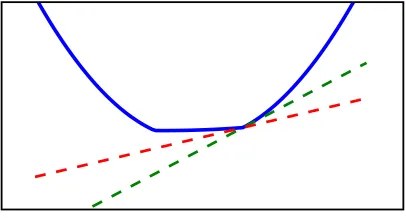
The precursor to the bundle methods is the cutting plane method (CPM) (Kelly, 1960). CPM uses subgradients, which are a generalization of gradients appropriate for convex functions, including those which are not necessarily smooth. Suppose w′ is a point where a convex function J is finite. Then a subgradient is the normal vector of any tangential supporting hyperplane of J at w′ (see Figure 1 for geometric intuition). Formally s′is called a subgradient of J at w′if, and only if,

J(w)_≥J(w′) +w−w′,s′ ∀w. (3)

The set of all subgradients at w′is called the subdifferential, and is denoted by∂wJ(w′). If this set is not empty then J is said to be subdifferentiable at w′. On the other hand, if this set is a singleton then the function is said to be differentiable at w′. Convex functions are subdifferentiable everywhere in their domain (Hiriart-Urruty and Lemar´echal, 1993).

As implied by (3), J is bounded from below by its linearization (i.e., first order Taylor approx-imation) at w′. Given subgradients s1,s2, . . . ,st evaluated at locations w0,w1, . . . ,wt−1, we can state

a tighter (piecewise linear) lower bound for J as follows

J(w)_≥J_tCP(w):=max

1≤i≤t{J(wi−1) +hw−wi−1,sii}. (4) This lower bound forms the basis of the CPM, where at iteration t the set{wi}ti−=01is augmented by

wt:=argmin w

J_tCP(w).

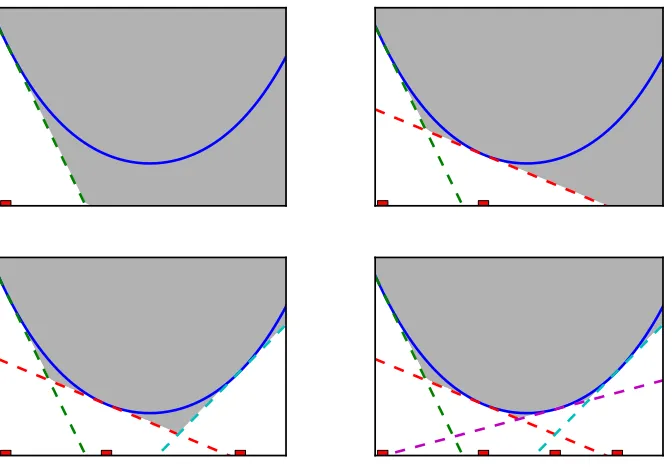
This iteratively refines the piecewise linear lower bound JCPand allows us to get close to the mini-mum of J (see Figure 2 for an illustration).

If w∗denotes the minimizer of J, then clearly each J(wi)≥J(w∗)and hence min0≤i≤tJ(wi)≥ J(w∗). On the other hand, since J ≥J_tCP it follows that J(w∗)_≥J_tCP(wt). In other words, J(w∗) is sandwiched between min0_≤i_≤tJ(wi) and JtCP(wt) (see Figure 3 for an illustration). The CPM monitors the monotonically decreasing quantity

εt := min

0≤i≤tJ(wi)−J

CP

t (wt),

and terminates wheneverεtfalls below a predefined thresholdε. This ensures that the solution J(wt) satisfies J(wt)≤J(w∗) +ε.

Figure 1: Geometric intuition of a subgradient. The nonsmooth convex function (solid blue) is only subdifferentiable at the “kink” points. We illustrate two of its subgradients (dashed green and red lines) at a “kink” point which are tangential to the function. The normal vectors to these lines are subgradients.

2.1 Standard Bundle Methods

Although CPM was shown to be convergent (Kelly, 1960), it is well known (see, e.g., Lemar´echal et al., 1995; Belloni, 2005) that CPM can be very slow when new iterates move too far away from the previous ones (i.e., causing unstable “zig-zag” behavior in the iterates).

Bundle methods stabilize CPM by augmenting the piecewise linear lower bound (e.g., J_tCP(w)

as in (4)) with a prox-function (i.e., proximity control function) which prevents overly large steps in the iterates (Kiwiel, 1990). Roughly speaking, there are 3 popular types of bundle methods, namely, proximal (Kiwiel, 1990), trust region (Schramm and Zowe, 1992), and level set (Lemar´echal et al., 1995).2 All three versions use 1_2k·k2as their prox-function, but differ in the way they compute the

Figure 2: A convex function (blue solid curve) is bounded from below by its linearizations (dashed lines). The gray area indicates the piecewise linear lower bound obtained by using the linearizations. We depict a few iterations of the cutting plane method. At each iteration the piecewise linear lower bound is minimized and a new linearization is added at the minimizer (red rectangle). As can be seen, adding more linearizations improves the lower bound.

Figure 3: A convex function (blue solid curve) with three linearizations (dashed lines) evaluated at three different locations (red squares). The approximation gapε3 at the end of third

new iterate:

proximal: wt:=argmin

w {

ζt

2kw−wˆt−1k 2

+J_tCP(w)_}, (5)

trust region: wt:=argmin

w {

J_tCP(w)_| 1_2kw₋wˆt₋1k2≤κt}, (6) level set: wt:=argmin

w {

1

2kw−wˆt−1k 2

|J_tCP(w)_≤τt},

where ˆwt₋1 is the current prox-center, andζt,κt, andτt are positive trade-off parameters of the stabilization. Although (5) can be shown to be equivalent to (6) for appropriately chosenζt and κt, tuningζt is rather difficult while a trust region approach can be used for automatically tuning κt. Consequently the trust region algorithmBTof Schramm and Zowe (1992) is widely used in practice.

Since our methods (see Section 2.2) are closely related to the proximal bundle method, we will now describe them in detail. Similar to the CPM the proximal bundle method also builds a piecewise linear lower bound J_tCP (see (4)). In contrast to the CPM, the piecewise linear lower bound augmented with a stabilization termζt

2 kw−wˆt−1k

2_{, is minimized to produce the intermediate}

iterate ¯wt. The approximation gap in this case includes the prox-function:

εt:=J(wˆt−1)−

J_tCP(w¯t) + ζt

2 kw¯t−wˆt−1k

2

.

Ifεtis less than the pre-defined thresholdεthe algorithm exits. Otherwise, a line search is performed along the line joining ˆwt−1and ¯wtto produce the new iterate wt. If wt results in a sufficient decrease of the objective function then it is accepted as the new prox-center ˆwt; this is called a serious step. Otherwise, the prox-center remains the same; this is called a null step. Detailed pseudocode can be found in Algorithm 1.

If the approximation gapεt is smaller thanε, then this ensures that the solution J(wˆt−1)satisfies

J(wˆt−1)≤J(w) +ζ₂t kw−wˆt−1k2+εfor all w. In particular, if J(w∗)denotes the optimum as before,

then J(wˆt−1)≤J(w∗) +ζ₂t kw∗−wˆt−1k2+ε. Contrast this with the approximation guarantee of the

CPM, which does not involve the ζt

2kw∗−wˆt−1k 2

term.

Although the positive coefficient ζt is assumed fixed throughout the algorithm, in practice it must be updated after every iteration to achieve faster convergence, and to guarantee a good quality solution (Kiwiel, 1990). Same is the case forκt andτt in trust region and level set bundle methods, respectively. Although the update is not difficult, the procedure relies on other parameters which require careful tuning (Kiwiel, 1990; Schramm and Zowe, 1992; Lemar´echal et al., 1995).

In the next section, we will describe our method (BMRM) which avoids this problem. There are two key differences between BMRMand the proximal bundle method: Firstly, BMRM main-tains a piecewise linear lower bound of Remp(w) instead of J(w). Secondly, the the stabilizer (i.e.,

Algorithm 1 Proximal Bundle Method

1: input & initialization:ε_≥0,ρ_∈(0,1), w0, t←0, ˆw0←w0 2: loop

3: t_←t+1

4: Compute J(wt−1)and st∈∂wJ(wt−1)

5: Update model J_tCP(w):=max1≤i≤t{J(wi−1) +hw−wi−1,sii} 6: w¯t←argminwJtCP(w) +ζ2tkw−wˆt−1k

2 7: εt ←J(wˆt−1)−

h

J_tCP(w¯t) +ζ₂t kw¯t−wˆt−1k2 i

8: ifεt <εthen return ¯wt

9: Linesearch: ηt ←argminη_∈RJ(wˆt−1+η(w¯t−wˆt−1)) (if expensive, setηt =1) 10: wt←wˆt−1+ηt(w¯t−wˆt−1)

11: if J(wˆt₋1)−J(wt)≥ρεt then 12: SERIOUS STEP: ˆwt ←wt 13: else

14: NULL STEP: ˆwt←wˆt₋1 15: end if

16: end loop

2.2 Bundle Methods for Regularized Risk Minimization (BMRM)

Define:

(subgradient of Remp) at∈∂wRemp(wt−1),

(offset) bt:=Remp(wt₋1)− hwt₋1,ati, (piecewise linear lower bound of Remp) RtCP(w):=max

1≤i≤t{hw,aii+bi}, (piecewise convex lower bound of J) Jt(w):=λΩ(w) +RtCP(w),

(iterate) wt :=min w Jt(w), (approximation gap) εt:= min

0≤i≤tJ(wi)−Jt(wt).

We now describeBMRM (Algorithm 2), and contrast it with the proximal bundle method. At it-eration t the algorithm builds the lower bound R_tCPto the empirical risk Remp. The new iterate wt is then produced by minimizing Jt which is RtCPaugmented with the regularizerΩ; this is the key difference from the proximal bundle method which uses the ζt

2 kw−wˆt−1k 2

prox-function for stabi-lization. The algorithm repeats until the approximation gapεt is less than the pre-defined threshold ε. Unlike standard bundle methods there is no notion of a serious or null step in our algorithm. In fact, our algorithm does not even maintain a prox-center. It can be viewed as a special case of standard bundle methods where the prox-center is always the origin and never updated (hence every step is a null step). Furthermore, unlike the proximal bundle method, the approximation guarantees of our algorithm do not involve the ζt

2 kw∗−wtk 2

term.

Algorithm 2BMRM

1: input & initialization:ε_≥0, w0, t←0 2: repeat

3: t_←t+1

4: Compute at ∈∂wRemp(wt−1)and bt←Remp(wt−1)− hwt−1,ati 5: Update model: RCP_t (w):=max1≤i≤t{hw,aii+bi}

6: wt←argminwJt(w):=λΩ(w) +RCPt (w) 7: εt ←min0≤i≤tJ(wi)−Jt(wt)

8: untilεt≤ε 9: return wt

observed by Franc and Sonnenburg (2008) in the case of linear SVMs with binary hinge loss.3 We now turn to a variant ofBMRMwhich uses a line search (Algorithm 3); this is a generalization of the optimized cutting plane algorithm for support vector machines (OCAS) of Franc and Sonnenburg (2008). This variant first builds R_tCPand minimizes Jt to obtain an intermediate iterate wt. Then, it performs a line search along the line joining wb_t−1and wtto produce wbt which acts like the new prox-center. Note that wt−wbt−1is not necessarily a direction of descent; therefore the line search might

return a zero step. Instead of using wb_t as the new iterate the algorithm uses the pre-set parameter θto generate wc_t on the line segment joining wb_t and wt. Franc and Sonnenburg (2008) report that settingθ=0.9 works well in practice. It is easy to see that Algorithm 3 reduces to Algorithm 2 if we setηt =1 for all t, and use the same termination criterion. It is worthwhile noting that this variant is not applicable for structured learning problems such as Max-Margin Markov Networks (Taskar et al., 2004), because no efficient line search is known for such problems.

A specialized variant of BMRMwhich handles quadratic regularizers, that is, Ω(w) =1_2kw_k2 was first introduced to the machine learning community by Tsochantaridis et al. (2005) asSVMstruct. In particular,SVMstruct handles quadratic regularizersΩ(w) = 1

2kwk

2 _{and non-differentiable large}

margin loss functions such as (24). Its 1-slack formulation (Joachims et al., 2009) can be shown to be equivalent toBMRMfor this specific type of regularizer and loss function. Somewhat confusingly, these algorithms are called the cutting plane method even though they are closer in spirit to bundle methods.

2.3 Dual Problems

In this section, we describe how the sub-problem

wt=argmin w

Jt(w):=λΩ(w) +max

1≤i≤thw,aii+bi (7) in Algorithms 2 and 3 is solved via a dual formulation. In fact, we will show that we need not know Ω(w)at all, instead it is sufficient to work with its Fenchel dual (Hiriart-Urruty and Lemar´echal, 1993):

Definition 1 (Fenchel Dual) Denote byΩ:

W

W

Ω∗_{(µ):= sup} w∈Wh

w,µ_{i −}Ω(w). (8)

Algorithm 3BMRMwith Line Search

1: input & initialization:ε_≥0,θ_∈(0,1], wb₀, wc_0←wb₀, t_←0

2: repeat 3: t_←t+1

4: Compute at ∈∂wRemp(wtc₋1), and bt ←Remp(wct₋1)−

wc_t−1,at

5: Update model: RCP_t (w):=max1_≤i_≤t{hw,aii+bi} 6: wt←argminwJt(w):=λΩ(w) +RCPt (w)

7: Linesearch: ηt ←argmin_η∈RJ(wbt₋1+η(wt−wbt₋1)) 8: wb_{t ←}wb_t−1+ηt(wt−wb_t−1)

9: wc_{t ←}(1₋θ)wb_t +θwt 10: ε_t ←J(wb

t)−Jt(wt) 11: untilεt≤ε

12: return w_tb

Several choices of regularizers are common. For

W

Ω(w) = 1

2kwk

2

2 and Ω∗(µ) =

1 2kµk

2 2.

More generally, for Lp norms one obtains (Boyd and Vandenberghe, 2004; Shalev-Shwartz and Singer, 2006):

Ω(w) = 1

2kwk

2

p and Ω∗(µ) =

1 2kµk

2

q where 1 p+

1 q=1.

For any positive definite matrix B, we can construct a quadratic form regularizer which allows non-uniform penalization of the weight vector as:

Ω(w) = 1

2w

⊤_{Bw and Ω}∗_{(µ) =} 1

2µ ⊤_B−1_µ.

For the unnormalized negative entropy, where

W

+, we have

Ω(w) =

∑

w(i)log w(i) and Ω∗(µ) =

∑

exp µ(i).

For the normalized negative entropy, where

W

Ω(w) =

∑

w(i)log w(i) and Ω∗(µ) =log

∑

exp µ(i).

Theorem 2 Denote by A= [a1, . . . ,at]the matrix whose columns are the (sub)gradients, and let b= [b1, . . . ,bt]. The dual problem of

wt =argmin w∈Rd {

Jt(w):=max

1_≤i_≤thw,aii+bi+λΩ(w)} is (9) αt =argmax

α∈Rt {

J_t∗(α):=₋λΩ∗(₋λ−1_{Aα) +α}⊤_{b|α≥0, kαk}

1=1}. (10)

Furthermore, wt andαt are related by the dual connection wt=∂Ω∗(−λ−1Aαt).

Proof We rewrite (9) as a constrained optimization problem: minw,ξλΩ(w) +ξ subject to ξ≥

hw,aii+bi for i=1, . . . ,t. By introducing non-negative Lagrange multipliersαand recalling that 1t denotes the t dimensional vector of all ones, the corresponding Lagrangian can be written as

L(w,ξ,α) =λΩ(w) +ξ₋α⊤ξ1t−A⊤w−b

withα≥0, (11)

whereα_≥0 denotes that each component ofαis non-negative. Taking derivatives with respect toξ yields 1₋α⊤1t = 0. Moreover, minimization of L with respect to w implies solving maxw

w,₋λ−1_{Aα−Ω(w) =Ω}∗_(−λ−1_{Aα). Plugging both terms back into (11) we eliminate the}

primal variablesξand w.

SinceΩ∗is assumed to be twice differentiable and the constraints of (10) are simple, one can easily solve (10) with standard smooth optimization methods such as the penalty/barrier methods (No-cedal and Wright, 1999). Recall that for the square norm regularizerΩ(w) = 1_2kw_k2₂, commonly used in SVMs and Gaussian Processes, the Fenchel dual is given byΩ∗(µ) = 1

2kµk 2

2. The following

corollary is immediate:

Corollary 3 For quadratic regularization, that is,Ω(w) =1_2kw_k2₂, (10) becomes αt =argmax

α∈Rt {−

1

2λα⊤A⊤Aα+α⊤b|α≥0,kαk1=1}.

This means that for quadratic regularization the dual optimization problem is a quadratic program (QP) where the number of constraints equals the number of (sub)gradients computed previously. Since t is typically in the order of 10s to 100s, the resulting QP is very cheap to solve. In fact, we do not even need to know the (sub)gradients explicitly. All that is required to define the QP are the inner products between (sub)gradientsai,aj

.

2.4 Convergence Analysis

While the variants of bundle methods we proposed are intuitively plausible, it remains to be shown that they have good rates of convergence. In fact, past results, such as those by Tsochantaridis et al. (2005) suggest a slow O(1/ε2_{)rate of convergence. In this section we tighten their results and}

show an O(1/ε)rate of convergence for nonsmooth loss functions and O(log(1/ε))rates for smooth loss functions under mild assumptions. More concretely we prove the following two convergence results:

(b) Under the above conditions, if furthermore∂2_wJ(w)≤H, that is, the Hessian of J is bounded, we can show O(log(1/ε))rate of convergence.

For our convergence proofs we use a duality argument similar to those put forward in Shalev-Shwartz and Singer (2006) and Tsochantaridis et al. (2005), both of which share key techniques with Zhang (2003). Recall thatεt denotes our approximation gap, which in turn upper bounds how far away we are from the optimal solution. In other words, εt ≥min0≤i≤tJ(wi)−J∗, where J∗ denotes the optimum value of the objective function J. The quantityεt−εt+1can thus be viewed as

the “progress” made towards J∗in iteration t. The crux of our proof argument lies in showing that for nonsmooth loss functions the recurrenceεt−εt+1≥c·ε2t holds for some appropriately chosen constant c. The rates follow by invoking a lemma from Abe et al. (2001). In the case of the smooth losses we show thatεt−εt+1≥c′·εtthus implying an O(log(1/ε))rate of convergence.

In order to show the required recurrence, we first observe that by strong duality the values of the primal and dual problems (9) and (10) are equal at optimality. Hence, any progress in Jt+1can

be computed in the dual. Next, we observe that the solution of the dual problem (10) at iteration t, denoted byαt, forms a feasible set of parameters for the dual problem (10) at iteration t+1 by means of the parameterization(αt,0), that is, by paddingαt with a 0. The value of the objective function in this case equals Jt(wt).

To obtain a lower bound on the improvement due to Jt+1(wt+1)we perform a 1-d optimization

along((1₋η)αt,η)in (10). The constraintη∈(0,1)ensures dual feasibility. We will then bound this improvement in terms ofεt. Note that, in general, solving the dual problem (10) results in a increase which is larger than that obtained via the line search. The 1-d minimization is used only for analytic tractability. We now state our key theorem and prove it in Appendix B.

Theorem 4 Assume that max_{u∈∂wRemp(w)k}u_{k ≤}G for all w_∈dom J. Also assume that Ω∗ has bounded curvature, that is, ∂2_µΩ∗(µ)≤H∗ for all µ∈ {−λ−1_∑t+1

i=1αiai whereαi ≥0, ∀i and ∑t+1

i=1αi=1}. In this case we have

εt−εt+1≥ε₂t min(1,λεt/4G2H∗). (12) Furthermore, if∂2_wJ(w)≤H, then we have

εt−εt+1≥     

εt/2 ifεt>4G2H∗/λ λ/8H∗ if 4G2H∗/λ_≥εt ≥H/2 λεt/4HH∗ otherwise.

Theorem 5 Assume that J(w)_≥0 for all w. Under the assumptions of Theorem 4 we can give the following convergence guarantee for Algorithm 2. For anyε<4G2H∗/λthe algorithm converges to the desired precision after

n_≤log₂λJ(0) G2_H∗+

8G2H∗ λε −1

steps. Furthermore if the Hessian of J(w)is bounded, convergence to any ε≤H/2 takes at most the following number of steps:

n_≤log₂ λJ(0) 4G2_H∗+

4H∗

λ max

0,H₋8G2H∗/λ+4HH∗

λ log(H/2ε).

Several observations are in order: First, note that the number of iterations only depends logarithmi-cally on how far the initial value J(0)is away from the optimal solution. Compare this to the result of Tsochantaridis et al. (2005), where the number of iterations is linear in J(0).

Second, we have an O(1/ε) dependence in the number of iterations in the non-differentiable case, as opposed to the O(1/ε2_{)rates of Tsochantaridis et al. (2005). In addition to that, the}

conver-gence is O(log(1/ε))for continuously differentiable problems.

Note that whenever Remp is the average over many piecewise linear functions, Remp behaves

essentially like a function with bounded Hessian as long as we are taking large enough steps not to “notice” the fact that the term is actually nonsmooth.

Remark 6 ForΩ(w) =1 2kwk

2

the dual Hessian is exactly H∗=1. Moreover we know that H_≥λ since∂2_wJ(w)=λ+∂2_wRemp(w)

.

Effectively the rate of convergence of the algorithm is governed by upper bounds on the primal and dual curvature of the objective function. This acts like a condition number of the problem—for Ω(w) = 1

2w⊤Qw the dual isΩ∗(z) = 1 2z⊤Q−

1_{z, hence the largest eigenvalues of Q and Q}−1_would

have a significant influence on the convergence.

In terms ofλthe number of iterations needed for convergence is O(λ−1_{). In practice the iteration}

count does increase withλ, albeit not as badly as predicted. This is likely due to the fact that the empirical risk Rempis typically rather smooth and has a certain inherent curvature which acts as a

natural regularizer in addition to the regularization afforded byλΩ(w).

For completeness we also state the convergence guarantees for Algorithm 3 and provide a proof in Appendix B.3.

Theorem 7 Under the assumptions of Theorem 4 Algorithm 3 converges to the desired precisionε after

n_≤8G

2_H∗

λε

steps for anyε<4G2H∗/λ.

3. Implementation Issues

3.1 Solving theBMRMSubproblem (7) with Limited Memory Space

In Section 2.3 we mentioned the dual of subproblem (7) (i.e., (10)) which is usually easier to solve when the dimensionality d of the problem is larger than the number of iterations t required by

BMRMto reach desired precision ε. Although t is usually in the order of 102, a problem with d in the order of 106or higher may use up all memory of a typical machine to store the bundle, that is, linearizations _{(ai,bi)}, before the convergence is achieved.4 Here we describe a principled technique which controls the memory usage while maintaining convergence guarantees.

Note that at iteration t, before the computation for new iterate wt, Algorithm 2 maintains a bundle of t (sub)gradients _{ai}ti=1 of Remp computed at the locations {wi}ti−=01. Furthermore, the

Lagrange multipliers αt−1 obtained in iteration t−1 satisfy αt−1≥0 and ∑t_i−₌₁1α(_t−i)₁=1 by the

constraints of (10). We define the aggregated (sub)gradient ˆaI, offset ˆbI and Lagrange multiplier ˆ

α(I)

t−1as

ˆ aI:=

1

ˆ α(I)

t−1

∑

α(i)

t−1ai, ˆbI:=

1

ˆ α(I)

t−1

∑

α(i)

t−1bi, and αˆ

(I)

t−1:=

∑

i∈I α(i)

t−1,

respectively, where I⊆[t−1]is an index set (Kiwiel, 1983). Clearly, the optimality of (10) at the end of iteration t₋1 is maintained when a subset

n

(ai,bi,α(_t−i)₁)

o

i∈I is replaced by the aggregate (aˆI,ˆbI,αˆ(_t−I)₁))for any I⊆[t−1].

To obtain a new iterate wt via (10) with memory space for at most k linearizations, we can, for example, replace_{(ai,bi)}i∈I with(aˆI,ˆbI)where I= [t−k+1]and 2≤k≤t. Then, we solve a k-dimensional variant of (10) with A := [aˆI,at−k+2, . . . ,at], b := [ˆbI,bt−k+2, . . . ,bt], andα∈Rk. The optimum of this variant will be lower than or equal to that of (10) as the latter has higher degree of freedom than the former. Nevertheless, solving this variant with 2_≤k_≤t will still guarantee convergence (recall that our convergence proof only uses k=2). In the sequel we name the aforementioned number k as the “bundle size” since it indicates the number of linearizations the algorithm keeps.

For concreteness, we provide here a memory efficientBMRMvariant for the cases whereΩ(w) = 1

2kwk 2

2and k=2. We first see that the dual of subproblem (7) now reads:

η=argmax

0_≤η_≤1 − 1 2λ

aˆ_[t₋1]+η(at−aˆ[t₋1]) 2

2+ˆb[t−1]+η(bt−ˆb[t−1])

≡argmax

0≤η≤1 −

η

λaˆ⊤[t₋1](at−aˆ[t−1])−η

2

2λ

at−aˆ⊤_[t₋1] 2

+η(bt−ˆb[t−1]). (13)

Since (13) is quadratic inη, we can obtain the optimalηby setting the derivative of the objective in (13) to zero and clippingηin the range[0,1]:

η=min max 0,bt−ˆb[t−1]+w

⊤

t−1at+λkwt−1k2 1

λkat+λwt₋1k2

! ,1

!

(14)

4. In practice, we can remove those linearizations{(ai,bi)}whose Lagrange multipliersαiare 0 after solving (10).

where wt−1 =−1_λaˆ[t−1] by the dual connection. With the optimal η, we obtain the new primal

iterate wt= (1−η)wt₋1−(η/λ)at. Algorithm 4 lists the details. Note that this variant is simple to implement and does not require a QP solver.

Algorithm 4BMRMwith Aggregation of Previous Linearizations

1: input & initialization:ε_≥0, w0, t←1

2: Compute a1∈∂wRemp(w0), and b1←Remp(w0)− hw0,a1i 3: w1← −1_λa1

4: ˆb_[1]←b1 5: repeat 6: t←t+1

7: Compute at ∈∂wRemp(wt₋1)and bt←Remp(wt₋1)− hwt₋1,ati 8: Computeηusing Eq. (14)

9: wt←(1−η)wt−1−(η/λ)at 10: ˆb_[t]←(1₋η)ˆb[t−1]+ηbt

11: ε_t ←min0≤i≤tλ₂kwik2+Remp(wi)−λ₂kwtk2−ˆb[t] 12: untilεt≤ε

3.2 Parallelization

Algorithms 2, 3, and 4 the evaluation of Remp(w) (and ∂wRemp(w)) is cleanly separated from the

computation of new iterate and the choice of regularizer. If Rempis additively decomposable over

the examples(xi,yi), that is, can be expressed as a sum of some independent loss terms l(xi,yi,w), then we can parallelize these algorithms easily by splitting the data sets and the computation Remp

over multiple machines. This parallelization scheme not only reduces the computation time but also allows us to handle data set with size exceeding the memory available on a single machine.

Without loss of generality, we describe a parallelized version of Algorithm 2 here. Assume there are p slave machines and 1 master machine available. At the beginning, we partition a given data set D=_{(xi,yi)}mi=1 into p disjoint sub-datasets{Di}ip=1 and assign one sub-dataset to each

slave machine. At iteration t, the master first broadcasts the current iterate wt−1 to all p slaves

(e.g., using MPI functionMPI::BroadcastGropp et al. 1999). The slaves then compute the losses and (sub)gradients on their local sub-datasets in parallel. As soon as the losses and (sub)gradients computation finished, the master combines the results (e.g., using MPI::AllReduce). With the combined (sub)gradient and offset, the master computes the new iterate wt as in Algorithms 2 and 3. This process repeats until convergence is achieved. Detailed pseudocode can be found in Algo-rithm 5.

4. Related Research

rank-Algorithm 5 ParallelBMRM

1: input:ε_≥0, w0, data set D, number of slave machines p

2: initialization: t_←0, assign sub-dataset Dito slave i, i=1, . . . ,p 3: repeat

4: t_←t+1

5: Master: Broadcast wt−1to all slaves

6: Slaves: Computes Ri_emp(wt−1):=∑(x,y)∈Dil(x,y,wt−1)and a

i

t∈∂wRiemp(wt−1) 7: Master: Aggregate at :=_|D1_|∑_ip₌₁ait and bt := _|D1_|∑_ip₌₁Riemp(wt₋1)− hwt₋1,ati 8: Master: Update model R_tCP(w):=max1≤j≤t{

w,aj

+bj} 9: Master: wt←argminwJt(w):=λΩ(w) +RCPt (w)

10: Master:εt ←min0≤i≤tJ(wi)−Jt(wt) 11: untilεt≤ε

12: return wt

ing (Crammer and Singer, 2005), maximization of multivariate performance measures (Joachims, 2005), structured estimation (Taskar et al., 2004; Tsochantaridis et al., 2005), Gaussian Process regression (Williams, 1998), conditional random fields (Lafferty et al., 2001), graphical models (Cowell et al., 1999), exponential families (Barndorff-Nielsen, 1978), and generalized linear mod-els (Fahrmeir and Tutz, 1994).

Traditionally, specialized solvers have been developed for solving the kernel version of (1) in the dual (see, e.g., Chang and Lin, 2001; Joachims, 1999). These algorithms construct the La-grange dual, and solve for the LaLa-grange multipliers efficiently. Only recently, research focus has shifted back to solving (1) in the primal (see, e.g., Chapelle, 2007; Joachims, 2006; Sindhwani and Keerthi, 2006). This spurt in research interest is due to three main reasons: First, many interesting problems in diverse areas such as text classification, word-sense disambiguation, and drug design already employ rich high dimensional data which does not necessarily benefit from the kernel trick. All these domains are characterized by large data sets (with m in the order of a million) and very sparse features (e.g., the bag of words representation of a document). Second, efficient factorization methods (e.g., Fine and Scheinberg, 2001) can be used for a low rank representation of the kernel matrix thereby effectively rendering the problem linear. Third, approximation methods such as the Random Feature Map proposed by Rahimi and Recht (2008) can efficiently approximate a infinite dimensional nonlinear feature map associated to a kernel by a finite dimensional one. Therefore our focus on the primal optimization problem is not only pertinent but also timely.

The widely usedSVMstructoptimizer of Thorsten Joachims5is closely related toBMRM. While

BMRMcan handle many different regularizers and loss functions,SVMstructis mainly geared towards square norm regularizers and non-differentiable soft-margin type loss functions. On the other hand,

SVMstructcan handle kernels whileBMRMmainly focuses on the primal problem.

Our convergence analysis is closely related to Shalev-Shwartz and Singer (2006) who prove mistake bounds for online algorithms by lower bounding the progress in the dual. Although not stated explicitly, essentially the same technique of lower bounding the dual improvement was used by Tsochantaridis et al. (2005) to show polynomial time convergence of the SVMstruct algorithm. The main difference however is that Tsochantaridis et al. (2005) only work with a quadratic

jective function while the framework proposed by Shalev-Shwartz and Singer (2006) can handle arbitrary convex functions. In both cases, a weaker analysis led to O(1/ε2_{)rates of convergence for}

nonsmooth loss functions. On the other hand, our results establish a O(1/ε)rate for nonsmooth loss functions and O(log(1/ε))rates for smooth loss functions under mild technical assumptions.

Another related work isSVMperf(Joachims, 2006) which solves the SVM with linear kernel in linear time.SVMperffinds a solution with accuracyεin O(md/(λε2_{))time, where the m training}

pat-terns xi∈Rd. This bound was improved by Shalev-Shwartz et al. (2007) to ˜O(1/λδε)for obtaining an accuracy ofεwith confidence 1₋δ. Their algorithm,Pegasos, essentially performs stochastic (sub)gradient descent but projects the solution back onto the L2ball of radius 1/

√

λ. Note that

Pe-gasosalso can be used in an online setting. This, however, only applies whenever the empirical risk

decomposes into individual loss terms (e.g., it is not applicable to multivariate performance scores Joachims 2005).

The third related strand of research considers gradient descent in the primal with a line search to choose the optimal step size (see, e.g., Boyd and Vandenberghe, 2004, Section 9.3.1). Under assumptions of smoothness and strong convexity – that is, the objective function can be upper and lower bounded by quadratic functions – it can be shown that gradient descent with line search will converge to an accuracy ofεin O(log(1/ε))steps. Our solver achieves the same rate guarantees for smooth functions, under essentially similar technical assumptions.

We would also like to point out connections to subgradient methods (Nedich and Bertsekas, 2000). These algorithms are designed for nonsmooth functions, and essentially choose an arbitrary element of the subgradient set to perform a gradient descent like update. Let max_{u∈∂wJ(w)k}u_{k ≤} G, and B(w∗,r) denote a ball of radius r centered around the minimizer of J(w). By applying the analysis of Nedich and Bertsekas (2000) to the regularized risk minimization problem with Ω(w):= λ_2kw_k2, Ratliff et al. (2007) show that subgradient descent with a fixed, but sufficiently small, stepsize will converge linearly to B(w∗,G/λ).

Finally, several papers (Keerthi and DeCoste, 2005; Chapelle, 2007) advocate the use of Newton-like methods to solve Support Vector Machines in the “primal”. However, they need to take precau-tions when dealing with the fact that the soft-margin type of loss funcprecau-tions such as the hinge loss is only piecewise differentiable. Instead, our method only requires subdifferentials, which always ex-ist for convex functions, in order to make progress. The large number of and variety of implemented problems shows the flexibility of our approach.

5. Experiments

In this section, we examine the convergence behavior ofBMRMand show that it is versatile enough to solve a variety of machine learning problems. All our experiments were carried out on a cluster of 24 machines each with a 2.4GHz AMD Dual Core processor and 4GB of RAM. Details of the loss functions, data sets, competing solvers and experimental objectives are described in the following subsections.

5.1 Convergence Behavior

training of a linear SVM with binary hinge loss:6

min

w J(w):= λ 2kwk

2₊1

m m

∑

max(0,1₋yihw,xii). (15)

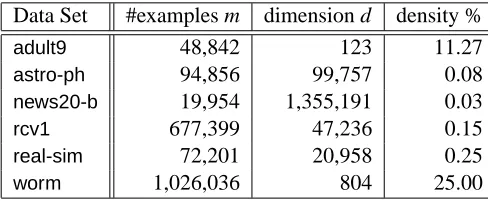
The experiments were conducted on 6 data sets commonly used in binary classification studies, namely, adult9, astro-ph, news20-b,7 rcv1, real-sim, andworm. adult9, news20-b, rcv1, and real-simare available on the LIBSVM tools website.8 astro-ph(Joachims, 2006) andworm(Franc and Sonnenburg, 2008) are available upon request from Thorsten Joachims and Soeren Sonnenburg, respectively. Table 1 summarizes the properties of the data sets.

Data Set #examples m dimension d density %

adult9 48,842 123 11.27

astro-ph 94,856 99,757 0.08

news20-b 19,954 1,355,191 0.03

rcv1 677,399 47,236 0.15

real-sim 72,201 20,958 0.25

worm 1,026,036 804 25.00

Table 1: Properties of the binary classification data sets used in our experiments.

5.1.1 REGULARIZATIONCONSTANTλANDAPPROXIMATION GAPε

As suggested by the convergence analysis, the linear SVM with the nonsmooth binary hinge loss should converge in O(1

λε)iterations, whereλandεare two parameters which one normally tunes

during the model selection phase. Therefore, we investigated the scaling behavior of our method w.r.t. these two parameters. We performed the experiments with unlimited bundle size and with a heuristic that removes subgradients which remained inactive (i.e., Lagrange multiplier = 0) for 10 or more consecutive iterations.9

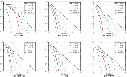
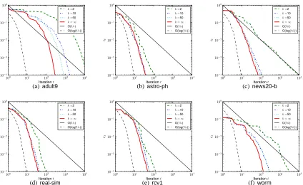
Figure 4 shows the approximation gapεt as a function of number of iterations t. As predicted by our convergence analysis,BMRMconverges faster for larger values ofλ. Furthermore, the empirical convergence curves exhibit a O(log(1/ε))rate instead of the (pessimistic) theoretical rate of O(1

ε),

especially for large values ofλ. Interestingly,BMRMconverges faster on high-dimensional text data sets (i.e.,astro-ph, news20-b, rcv1, andreal-sim) than on lower dimensional data sets (i.e.,adult9

andworm).

5.1.2 BUNDLESIZE

The dual of our method (10) is a concave problem which has dimensionality equal to the number of iterations executed. In the case of linear SVM, (10) is a QP. Hence, as described in Section 3.1, we can trade potentially greater bundle improvement for memory efficiency.

6. Similar behavior was observed with other loss functions.

7. The data set is originally namednews20; we renamed it to avoid confusion with the multiclass version of the data set.

(a)adult9 (b)astro-ph (c)news20-b

(d)real-sim (e) rcv1 (f) worm

Figure 4: Approximation gapεt as a function of number of iterations t; for different regularization constantsλ(and unlimited bundle size).

Figure 5 shows the approximation gapεt during the training of linear SVM as a function of the number of iterations t, for different bundle sizes k_{∈ {}2,10,50,∞_}. In the case of k=∞, we em-ployed the same heuristics which remove inactive linearizations as those mentioned in Section 5.1.1. As expected, the larger k is, the faster the algorithm converges. Although the case k=2 is the slow-est, its convergence rate is still faster than the theoretical bound _λε1.

5.1.3 PARALLELIZATION

When the empirical risk Rempis additively decomposable, the loss and subgradient computation can

be executed concurrently on multiple processors for different subsets of data points.10

We performed experiments for linear SVMs training with parallelized risk computation on the

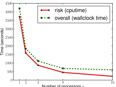
wormdata set. Figure 6(a) shows the wallclock time for the overall training phase (e.g., data loading, risk computation, and solving the QP) and CPU time for just the risk computation as a function of number of processors p. Note that the gap between the two curves essentially tells the runtime upper bound of the sequential part of the algorithm. As expected, both overall and risk computation time decrease as the number of processors p increases. However, in Figure 6(b), we see two different speedups.11 The speedup for the risk computation is roughly linear as there is no sequential part in

10. This requires only slight modification to the data loading process and the addition of some parallelization related code before and after the code segment for empirical risk computation.

11. Speedup Sp= TT1p where p is the number of processors and Tq is the runtime of the parallelized algorithm on q

(a)adult9 (b)astro-ph (c)news20-b

(d)real-sim (e) rcv1 (f) worm

Figure 5: Approximation gapεt as a function of number of iterations t; for different bundle sizes k (and fixed regularization constantλ=10−4).

it; the speedup of overall computation is approaching a limit12as well-explained by Amdahl’s law (Amdahl, 1967).

5.1.4 GENERALIZATIONVERSUSAPPROXIMATIONGAP

Since the problems we are considering are convex, all properly convergent optimizers will converge to the same solution. Therefore, comparing generalization performance of the final solution is mean-ingless. But, in real life one is often interested in the speed with which the algorithm achieves good generalization performance. In this section we study this question. We focus on the generalization (in terms of accuracy) as a function of approximation gap during training. For this experiment, we randomly split each of the data sets into training (60%), validation (20%) and testing (20%) sets.

We first obtained the bestλ_{∈ {}2−20_{, . . . ,2}0_{}for each of the data sets using their corresponding}

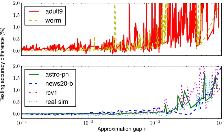
validation sets. With these bestλ’s, we (re)trained linear SVMs and recorded the testing accuracy as well as the approximation gap at every iteration, with termination criterionε=10−4. Figure 7 shows the difference between the testing accuracy evaluated at every iteration and that after training, as a function of approximation gap at each iteration.

From the figure, we see that the testing accuracies foradult9andwormdata sets are less stable in general and the approximation gap must be reduced to at least 10−3 to reach the 0.5% regime

(a) Risk computation in CPU time (red solid line) and over-all computation (i.e., data loading + risk computation + solving the QP) in wallclock time (green dashed line) as a function of number of processors.

(b) Speedup in risk computation (in CPU time) and overall computation (in wallclock time) as a function of number of processors.

Figure 6: CPU and wallclock time for training linear SVM using parallelBMRMonwormdata set with varying number of processors p_{∈ {}1,2,4,8,16_}. In these experiments, regulariza-tion constantλ=10−6_{, and termination criterion}ε₌₁₀−4_.

of the final testing accuracies; the testing accuracies for the rest of the data sets arrived at the same regime with approximation gap of 10−2or lower.

In general, the generalization improved as the approximation gap decreased. The improvement in generalization became rather insignificant (say, the maximum of changes in testing accuracies is less than 0.1%) when the approximation gap was further reduced to below some effective threshold εeff; that said, it is not necessary to continue the optimization whenεt ≤εeff.13 Since εeff (or its

scale) is not known a priori and the asymptotic analysis in Shalev-Schwartz and Srebro (2008) does not reveal the actual scale ofεeff directly applicable in our case, we carried out another set of

experiments to investigate ifεeff could be estimated with as little effort as possible: For each data

set, we randomly subsampled 10%, . . . ,50% of the training set as sub-datasets and performed the same experiment on all sub-datasets. We then determined the largestεeff such that the maximum

changes in testing accuracies is less than 0.1%.

Table 5.1.4 shows the (base 10 logarithm of)εefffor all sub-datasets as well as the full data sets.

It seems that theεeffestimated on a smaller sub-dataset is at most 1 order of magnitude larger than

the actualεeffrequired on full data set. In addition, we show in the table that the necessary threshold

ε10%required by the sub-datasets and the full data sets to attain the final testing accuracies attained

by the 10% sub-datasets. The observations obey the analysis in Shalev-Schwartz and Srebro (2008) that for a fixed testing accuracy, approximation gap (i.e., optimization error) can be relaxed when more data is given.

Figure 7: Difference between testing accuracies of intermediate and final models.

5.2 Comparison with Existing Bundle Methods

In this section we compare BMRMwith aBTimplementation obtained from Schramm and Zowe (1992).14 _{We also compare the performance ofBMRM(Algorithm 2) andLSBMRM(Algorithm 3).}

The multiclass line search used inLSBMRMcan be found in Yu et al. (2008).

For binary classification, we solve the linear SVM (15) on the data sets: adult9, astro-ph,

news20-b, rcv1, real-sim, and worm as mentioned in Section 5.1. For multiclass classification,

we solve (Crammer and Singer, 2003):

min

w J(w):= λ 2kwk

2₊ 1

m m

∑

max y′

i∈[c]

D

w,e_y′

i⊗xi−eyi⊗xi

E

+I(yi6=y′i), (16)

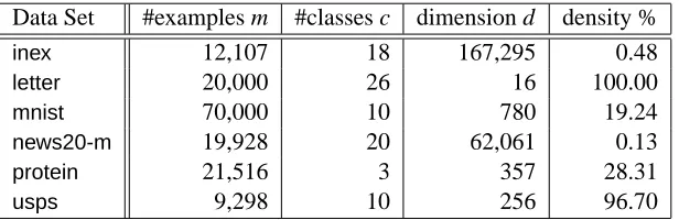
where c is the number of classes in the problem, ei is the i-th standard basis for Rc, ⊗ denotes Kronecker product; and I(_·)is an indicator function that has value 1 if its argument is evaluated true, and 0 otherwise. The data sets used in multiclass classification experiments wereinex,letter,mnist,

news20-m,15protein, andusps. inexis available for download on the website of Antoine Bordes16

and the rest can be found on the LIBSVM tools website.17 Table 3 summarizes the properties of these data sets.

In each of the experiments, we first obtain the optimal weight vector ¯w by runningBMRMuntil the termination criteria J(wt)−Jt(wt)≤0.01J(wt) is satisfied. Then we run BT, LSBMRM, and

14. The original FORTRAN implementation was automatically converted into C for use in our library.

15. The data set is originally namednews20; we renamed it to avoid confusion with the binary version of the data set. 16. Software available athttp://webia.lip6.fr/˜bordes/datasets/multiclass/inex.tar.gz.

10% 20% 30% 40% 50% 100%

adult9

Acc. (%) 84.3 84.7 84.9 85.1 85.1 85.2 log₁₀εeff -3.90 -3.72 -3.77 -3.88 -3.64 -4.00

log₁₀ε10% -4.01 -1.18 -1.07 -1.16 -1.27 -1.04

astro-ph

Acc. (%) 96.1 96.6 96.4 96.6 96.8 97.4 log₁₀εeff -1.48 -1.70 -1.57 -1.49 -1.68 -1.84

log₁₀ε10% -4.00 -1.15 -1.06 -0.98 -1.02 -0.87

news20-b

Acc. (%) 89.9 92.9 94.3 94.5 95.4 96.6 log₁₀εeff -2.00 -2.48 -3.87 -1.65 -3.71 -2.84

log₁₀ε10% -4.02 -0.92 -0.70 -0.80 -0.80 -0.67

rcv1

Acc. (%) 96.9 97.2 97.4 97.2 97.5 97.6 log₁₀εeff -2.02 -2.40 -1.99 -2.16 -2.34 -2.28

log₁₀ε10% -4.07 -1.19 -1.30 -1.29 -1.13 -1.11

real-sim

Acc. (%) 95.0 95.9 96.3 96.6 96.6 97.2 log₁₀εeff -1.74 -1.84 -1.71 -1.99 -1.74 -1.75

log₁₀ε10% -4.02 -1.04 -0.88 -0.87 -0.85 -0.82

worm

Acc. (%) 98.2 98.2 98.2 98.3 98.3 98.4 log₁₀εeff -2.43 -2.47 -2.48 -3.62 -2.81 -3.55

log₁₀ε10% -4.00 -1.38 -1.28 -1.37 -1.28 -1.31

Table 2: The first sub-row in each data set row indicates the testing accuracies of models trained on the corresponding proportions of the training set. The second sub-row indicates the (base 10 logarithm of) effective threshold such that the maximum difference in testing accuracies of models with approximation gap smaller than that is less than 0.1%. The third sub-row indicates the (base 10 logarithm of) threshold necessary for models to attain the testing accuracy attained by the model trained on the 10% sub-dataset with defaultε=10−4.

Data Set #examples m #classes c dimension d density %

inex 12,107 18 167,295 0.48

letter 20,000 26 16 100.00

mnist 70,000 10 780 19.24

news20-m 19,928 20 62,061 0.13

protein 21,516 3 357 28.31

usps 9,298 10 256 96.70

Table 3: Properties of the multiclass classification data sets used in the experiments.

BMRMuntil the following termination criteria is satisfied:

J(wt)−J(w¯)≤0.01J(w¯). (17)

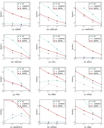
Figure 8 shows the number of iterations t required by the three methods on each data set to satisfy (17) as a function of regularization constant λ_∈10−3_,10−4_,10−5_,10−6 _{. As expected,}

LSBMRM, which uses an exact line search, outperformed bothBMRMandBTon all data sets.BMRM

AlthoughBTtunes the stabilization trade-off parameterκt automatically, it still does not guarantee superiority overBMRMwhich is considerably simpler. Nevertheless, external stabilization (inBT) clearly helps speed up the convergence in certain cases.

5.3 Versatility

In the following subsections, we will illustrate some of the applications ofBMRMto various machine learning problems with smooth and non-differentiable loss functions, and with different regularizers. Our aim is to show thatBMRM is versatile enough to be used in a variety of seemingly different problems. Readers not interested in this aspect ofBMRMcan safely skip this subsection.

5.3.1 BINARYCLASSIFICATION

In this section, we evaluate the performance of our methodBMRMin the training of binary classifier using linear SVMs (15) and logistic loss:

min

w J(w):= λ 2kwk

2₊ 1

m m

∑

log(1+exp(₋yihw,xii)),

on the binary classification data sets mentioned in Section 5.1 with split similar to that in Sec-tion 5.1.4. Since we will compareBMRMwith other solvers which use different termination crite-ria, we consider the CPU time used in reducing the relative difference between the current smallest objective function value and the optimum:

mini≤tJ(wi)−J(w∗) J(w∗₎ ,

where wiis the weight vector at time/iteration i, and w∗is the minimizer obtained by runningBMRM until the approximation gapεt <10−4. The bestλ∈

2−20, . . . ,20 for each of the data sets was determined by evaluating the performance on the corresponding validation set.18

In the case of linear SVMs, we comparedBMRMto three publicly available state of the art batch learning solvers:

1. OCAS (Franc and Sonnenburg, 2008). Since this method is equivalent to LSBMRM with binary hinge loss, we refer to this software byLSBMRMfor naming consistency.

2. LIBLINEAR(Fan et al., 2008) version 1.33 with option “-s 3”.

3. SVMperf(Joachims, 2006) version 2.5 with option “-w 3” and with double precision floating point numbers.

LIBLINEARsolves the dual problem of linear SVM using a coordinate descent method (Hsieh et al.,

2008). SVMperfwas chosen for comparison as it is algorithmically identical toBMRMin this case.

BothLIBLINEARandSVMperfprovide a “shrinking” technique to speed up the algorithms by

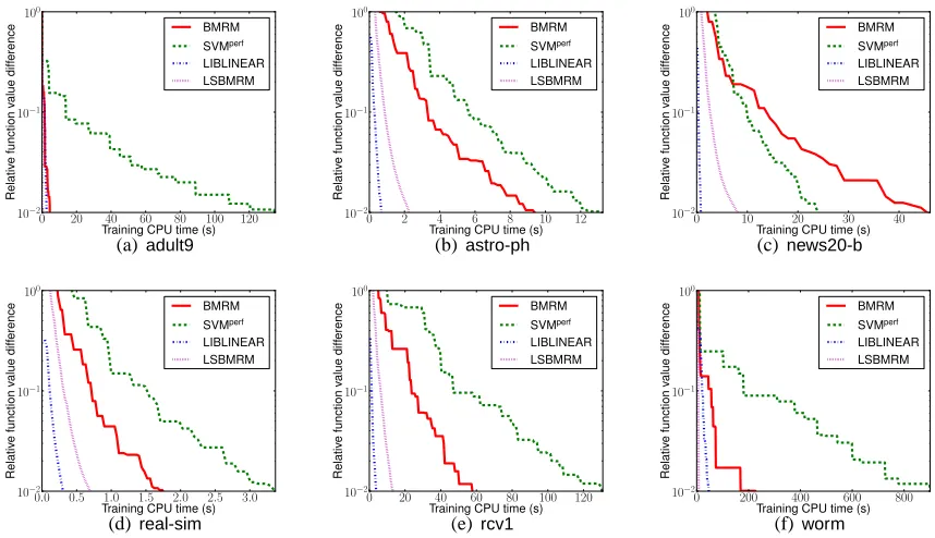
ignor-ing some data points which are not likely to affect the objective. SinceBMRMdoes not provide such shrinking technique, we excluded this option in bothLIBLINEARandSVMperffor a fair comparison. Figure 9 shows the relative difference in objective value as a function of training time (CPU seconds) for three methods on various data sets. BMRM is faster than SVMperf on all data sets

(a)adult9 (b)astro-ph (c)news20-b

(d)real-sim (e)rcv1 (f) worm

(g)inex (h)letter (i) mnist

(j)news20-m (k)protein (l)usps

Figure 8: Smallest number of iterations required to satisfy the termination criterion (17) for each data set and various regularization constants. (BTdid not satisfy (17) in theinexandusps

(a)adult9 (b)astro-ph (c)news20-b

(d)real-sim (e) rcv1 (f) worm

Figure 9: Linear SVMs. Relative primal objective value difference during training.

exceptnews20-b. The performance difference observed here is largely due to the differences in the implementations (e.g., feature vector representation, QP solver, etc.). Nevertheless, bothBMRMand

SVMperfare significantly outperformed byLSBMRMandLIBLINEARon all data sets, andLIBLINEAR

is almost always faster than LSBMRM. It is clear from the figure that LSBMRM and LIBLINEAR

enjoy progression with “strictly” decreasing objective values; whereas the progress of bothBMRM

andSVMperfare hindered by the “stalling” steps (i.e., the flat line segments in the plots). The fact

thatLSBMRMis different fromBMRMandSVMperfby one additional line search step implies that

the “stalling” steps is the time thatBMRMandSVMperfimprove the approximation at the regions which do not help reducing the primal objective function value.

In the case of logistic regression, we compareBMRMto the state of the art trust region Newton method for logistic regression (Lin et al., 2008) which is also available in theLIBLINEARpackage (option “-s 0”). From Figure 10, we see thatLIBLINEARoutperformsBMRMon all data sets and thatBMRMsuffers from the same “stalling” phenomenon as observed in the linear SVMs case.

5.3.2 LEARNING THECOSTMATRIXFORGRAPHMATCHING

(a)adult9 (b)astro-ph (c)news20-b

(d)real-sim (e) rcv1 (f) worm

Figure 10: Logistic regression. Relative primal objective value difference during training.

can be solved in worst case O(n3)time where n is the number of landmark points (Kuhn, 1955).19 Formally, the LAP reads

max y∈Y

n

∑

n

∑

yii′C_ii′,

where

Y

Cii′ :=−

d

∑

(k)

i −x′

(k)

i′

2

.

Instead of finding more features to describe the points xi and x′_i′ that might improve the matching results, Caetano et al. (2007) propose to learn a weighting to a given set of features that actually improved the matching results in many cases (Caetano et al., 2008).

In Caetano et al. (2007, 2008) the problem of learning the cost matrix for graph matching is formulated as a L2regularized risk minimization with loss function

l(x,x′,y,w) =max

¯

y∈Y

w,φ(x,x′,y¯)₋φ(x,x′,y)+∆(y¯,y), (18)

where the feature mapφis defined as

φ(x,x′,y) =₋ n

∑

n

∑

yii′(|x(1)_i −x′_i(1)_′ |2, . . . ,|x(_id)−x_i′(_′d)|2), (19)